LPT–Orsay 06/060

LAL–Orsay 06/144

hep-ph/0610173

October 2006

Abstract

It is notorious that, contrary to all other precision electroweak data, the forward–backward asymmetry for $b$ quarks $A_{FB}^{b}$ measured in $Z$ decays at LEP1 is nearly three standard deviations away from the predicted value in the Standard Model; significant deviations also occur in measurements of the asymmetry off the $Z$ pole. We show that these discrepancies can be resolved in a variant of the Randall–Sundrum extra–dimensional model in which the gauge structure is extended to ${\rm SU(2)_{L}\!\times\!SU(2)_{R}\!\times\!U(1)_{X}}$ to allow for relatively light Kaluza–Klein excitations of the gauge bosons. In this scenario, the fermions are localized differently along the extra dimension, in order to generate the fermion mass hierarchies, so that the electroweak interactions for the heavy third generation fermions are naturally different from the light fermion ones. We show that the mixing between the $Z$ boson with the Kaluza–Klein excitations allows to explain the $A_{FB}^{b}$ anomaly without affecting (and even improving) the agreement of the other precision observables, including the $Z\to b\bar{b}$ partial decay width, with experimental data. Some implications of this scenario for the ILC are summarized.

1. Introduction

The Standard Model (SM) of the strong and electroweak interactions of elementary particles [1] has brilliantly passed almost all the experimental tests to date. These tests, performed at the per–mille level accuracy, have probed the quantum corrections and the structure of the ${\rm SU(3)_{C}\times SU(2)_{L}\times U(1)_{Y}}$ local symmetry [2, 3]. However, it is notorious that there is an observable for which the measured value significantly differs from the one predicted in the context of the SM. The forward–backward (FB) asymmetry for $b$ quark jets $A_{FB}^{b}$ [4] measured in $Z$ boson decays at LEP1 provides, together with the longitudinal asymmetry $A_{LR}$ measured at the SLC, the most precise individual measurement of the electroweak mixing angle $\sin^{2}\theta^{\rm lep}_{\rm eff}$, but the result is 2.8 standard deviations away from the predicted value and the two individual measurements differ by more than three standard deviations. In fact, the $A_{FB}^{b}$ anomaly is present not only in the data collected at the $Z$ boson pole, but also a few GeV above and, to a lesser extent, a few GeV below the $Z$ pole. [There are also measurements of $A_{FB}^{b}$ at energies below (from PEP to TRISTAN) [5, 6, 7] and far above (LEP2) [8] the $Z$–pole which are in a reasonable agreement with the SM expectations.]

This situation has led to speculations about a possible signal of New Physics beyond the SM in the $Zb\bar{b}$ vertex. However, it turns out that this discrepancy cannot be easily explained without affecting the $Z\to b\bar{b}$ partial decay width, which has also been very precisely measured at LEP1 and found to be compatible with the SM expectation, and the FB longitudinal asymmetry $A_{FB,LR}^{b}$ measured at the SLC, although the corresponding experimental error is larger [3]. The basic reason for this difficulty lies in the fact that a very large correction, ${\cal O}(30\%)$, is needed to alter the initially small right–handed component of the $b$–quark coupling to $Z$ bosons without affecting significantly the left–handed $b$–quark coupling as well as the couplings of all other light fermions. Note that this large effect can possibly not be generated through radiative corrections in reasonable models [this is, for instance, the case in supersymmetric extensions of the SM where loop contributions of relatively light partners of the top quark and the $W$ boson [10] cannot account for the discrepancy] and one has to resort to large tree–level effects to explain the anomaly.

Several New Physics models fulfilling theses conditions have been proposed in the literature, though. Three examples of such models are variations of left–right symmetric models in which a new gauge boson $Z^{\prime}$ occurs and has interactions only with third generation fermions [11], models involving additional exotic (mirror) bottom–like quarks which strongly mix with the $b$–quarks [7, 12] and models where the electroweak symmetry breaking is induced by a new strongly interacting sector coupled to the SM fields [13]. In most of the models listed above, a kind of non–universality in which the third generation fermions are treated differently from the ones of the first and second generations is assumed. In most cases, this assumption is made in an ad–hoc way and specifically to cure the $A_{FB}^{b}$ anomaly.

Recently, it has been shown [14] that in different scenarios beyond the SM, such as Technicolor scenarios, Little Higgs theories, Higgsless models and models where the composite Higgs boson arises as a pseudo–Goldstone boson [which are related to theories in five–dimensional Anti-de-Sitter space via the AdS/CFT correspondence], one can invoke a custodial O(3) symmetry which protects at the same time the $\rho$ parameter and the $Zb_{L}\bar{b}_{L}$ coupling. Such an approach might also account for the required shift of the $Zb_{R}\bar{b}_{R}$ coupling to explain the $A_{FB}^{b}$ anomaly, if one allows for a deviation of the $Z\to b\bar{b}$ partial decay width; this point will be discussed later. The implications of this O(3) symmetry have been subsequently discussed within Higgsless models [15] and gauge-Higgs unification scenarios [16].

In this paper, we point out that the discrepancy between the measured value of $A_{FB}^{b}$ and the theoretical prediction can be resolved in the context of variants of the Randall–Sundrum (RS) extra–dimensional model [17] in which the fermion and bosonic fields are propagating in the bulk. These models, besides the fact that they explain the large hierarchy between the Planck and TeV scales without introducing any fundamentally new energy scale in the theory, allow for the unification of the gauge coupling constants at a high energy Grand Unification scale [18], provide a solution for proton decay and have a viable candidate of Kaluza–Klein type for the dark matter of the universe [19]. They also have the additional attractive feature of providing a geometrical explanation of the large mass hierarchies prevailing among SM fermions [20, 21, 22]. Indeed, when the SM fermions are localized differently along the extra dimension depending on their nature, their different wave functions which overlap with the Higgs boson [which is still localized on the TeV–brane for its mass to be protected] generate large hierarchical patterns among their effective four-dimensional Yukawa couplings. One can then naturally obtain electroweak interactions for the heavy third generation fermions that are different from the ones of the light fermions.

More specifically, we will work in a variant of the RS model proposed in Ref. [23] where the electroweak symmetry is enhanced to the left–right gauge symmetry ${\rm SU(2)_{L}\!\times\!SU(2)_{R}\!\times\!U(1)_{X}}$ in which the bulk fields are embedded, the right–handed fermions being promoted to ${\rm SU(2)_{R}}$ isodoublets. With this symmetry, the high–precision electroweak measurements can be nicely fitted while keeping the masses of the first Kaluza–Klein (KK) excitation modes of the gauge bosons rather low, $M_{KK}$ of order of a few TeV, which is required if the gauge hierarchy problem is to be addressed within the RS model with bulk matter. The ordinary $Z$ boson will then mix with its KK excitations and those of the new $Z^{\prime}$ boson, with the possibility of choosing their effective couplings in such a way that only the overall $Z$ couplings to third generation fermions are significantly altered. This would provide an explanation for the $A_{FB}^{b}$ anomaly, while keeping the electroweak observables involving light fermions as well as the $Z\to b\bar{b}$ decay width, unaltered for $M_{KK}={\cal O}$ (TeV). In this context, we propose two scenarios: one in which the U(1) group is ${\rm U(1)_{\rm B-L}}$ (as originally discussed in Ref. [23]) and a second in which the right–handed $b$–quark has isospin $I_{3R}^{b_{R}}\!=\!+\!\frac{1}{2}$ under the ${\rm SU(2)_{R}}$ group. While the $A_{FB}^{b}$ anomaly on the $Z$ pole is resolved in both scenarios, the experimental data for the asymmetry off the $Z$ pole are reproduced only in the second scenario.

The paper is organized as follows. In the next section, we briefly describe the extra–dimensional model of Ref. [23] based on the ${\rm SU(2)_{L}\times SU(2)_{R}\times U(1)_{X}}$ symmetry and summarize the main features which allow for relatively light KK states; the role of the fermions and their couplings to the $Z$ boson are then summarized. In section 3, we discuss two scenarios in which the choice of $Z$–fermion couplings allows to explain the $A_{FB}^{b}$ anomaly at energies on the $Z$ pole and reproduce the value of the $Z\to b\bar{b}$ partial decay width, without affecting the other precision measurements. In section 4, we analyze the asymmetry off the $Z$ pole and show that the agreement between theory and experiment is satisfactory only in the scenario where the right–handed $b$–quark has isospin $I_{3R}^{b_{R}}=+\frac{1}{2}$ under the ${\rm SU(2)_{R}}$ group. In section 5, we discuss the implications of this scenario at the ILC. A brief conclusion is presented in section 6.

2. The physical set–up

2.1 Theoretical framework

We consider the higher–dimensional Randall–Sundrum scenario in which the Standard Model fields are propagating in the bulk like gravity, except for the Higgs boson which remains confined on the TeV–brane in order not to re–introduce a gauge hierarchy. On the Planck–brane, the gravity scale is equal to the reduced Planck mass $M_{P}=2.44\times 10^{18}$ GeV, whereas the effective gravity scale on the TeV–brane, $M_{\star}=wM_{P}$, is suppressed by the exponential “warp” factor $w={\rm exp}(-\pi kR_{c})$ where $1/k$ is the curvature radius of the anti–de Sitter space and $R_{c}$ the compactification radius. For a small extra dimension, $R_{c}\simeq 11/k$ with $k$ being close to $M_{P}$, one finds $w\sim 10^{-15}$ so that $M_{\star}\!=\!{\cal O}(1)$ TeV, thus addressing the gauge hierarchy problem. For this $R_{c}$ value, the five–dimensional gravity scale $M_{5}$ is close to the effective four–dimensional gravity scale $M_{P}$.

The mass of the first Kaluza–Klein excitations of the SM gauge bosons, $M_{KK}=M_{\gamma^{(1)}}=M_{g^{(1)}}\approx M_{Z^{(1)}}\approx M_{W^{\pm(1)}}$, reads $M_{KK}=2.45kw=2.45kM_{\star}/M_{P}\sim M_{\star}={\cal O}$(TeV) and, since this parameter is more “physical”, we adopt it as our free input parameter instead of $k$. The maximal value of $M_{KK}$ is fixed by $kR_{c}$ and the theoretical consistency bound on the five–dimensional curvature scalar by $|R_{5}|=|-20k^{2}|<M_{5}^{2}$ leading to $k<0.105M_{P}$; one can thus take a maximal value of $M_{KK}\sim 10$ TeV which corresponds to the value $kR_{c}=10.11$. In fact, there exist a severe indirect bound of typically $M_{KK}\gtrsim 10$ TeV originating from electroweak precision data [24]. In order to soften this bound down to a few TeV and, thus, to allow for a solution of the gauge hierarchy problem, several scenarios have been proposed. For instance, scenarios with brane–localized kinetic terms for fermions and gauge bosons [25] allow to lower the previous bound down to a few TeV [26]. Another possibility, that we retain here, is the model of Agashe et al. [23] in which the electroweak gauge symmetry is enhanced to a left–right ${\rm SU(2)_{L}\times SU(2)_{R}\times U(1)_{X}}$ structure in the bulk and where right–handed fermions are promoted to ${\rm SU(2)_{R}}$ doublet fields, the new doublet components having no zero mode. The usual SM electroweak symmetry is recovered after the breaking of both ${\rm SU(2)_{R}}$ and ${\rm U(1)_{X}}$ on the Planck–brane, with possibly a small breaking of ${\rm SU(2)_{R}}$ in the bulk.

As mentioned in the introduction, the RS model with bulk matter provides naturally a geometrical interpretation of quark/lepton mass hierarchies [20]. The idea is to localize the SM fermions differently along the extra dimension, depending on their nature. Then, the overlapping of their different wave functions with the Higgs boson generates large hierarchical patterns among the effective four–dimensional Yukawa coupling constants. In this mass model, each five–dimensional fermion field $\Psi_{i}$ [$i=\{1,2,3\}$ is the family index in the interaction basis] couples to a distinct mass $m_{i}$ in the fundamental theory as $\int d^{4}x\int dy\sqrt{G}m_{i}\bar{\Psi}_{i}\Psi_{i}$ where $G$ is the determinant of the RS metric and $y$ parameterizes the fifth dimension. The localization of fermions along the extra dimension is fixed by the dependence of mass $m_{i}$ on $y$. One can take $m_{i}={\rm sign}(y)c_{i}k$ [27] where $c_{i}$ are dimensionless parameters. Then the fields decompose as $\Psi_{i}(x^{\mu},y)=\sum_{n=0}^{\infty}\psi_{i}^{(n)}(x^{\mu})f_{n}^{i}(y)$, with $n$ labeling the tower of KK excitations, admitting as a solution for the zero mode wave function $f_{0}^{i}(y)=\exp[(2-c_{i})k|y|]/N_{0}^{i}$, where $N_{0}^{i}$ is a normalization factor. The Yukawa interactions with the Higgs boson $H$ read then

$${\cal S}_{\rm Yukawa}=\int d^{5}x\sqrt{G}\left(Y_{ij}^{(5)}H\bar{\Psi}_{+i}\Psi_{-j}+{\rm h.c.}\right)=\int d^{4}xM_{ij}\bar{\psi}_{Li}^{(0)}\psi_{Rj}^{(0)}+{\rm h.c.}+\dots$$ (1)

where $Y_{ij}^{(5)}$ are the five–dimensional Yukawa coupling constants and the dots stand for KK mass terms. The effective fermion mass matrix is obtained after the integration

$$M_{ij}=\int dy\ \sqrt{G}\ Y_{ij}^{(5)}\ Hf_{0}^{i}(y)f_{0}^{j}(y).$$ (2)

The dimensionful $Y_{ij}^{(5)}$ couplings can be chosen almost universal so that the quark/lepton mass hierarchies are essentially generated through the overlap between $f_{0}^{i,j}(y)$ and $H$ along $y$. Remarkably, large fermion mass hierarchies can be created for fundamental parameters $m_{i}$ all of the order of the unique scale of the theory, $k\sim M_{5}\sim M_{P}$.

2.2 The couplings to fermions

Let us now discuss the fermions couplings to the $Z$ boson in the context of this extended left–right symmetric model. For each fermion $f_{L/R}$ of left/right–handed chirality, the couplings to the $Z$ boson which in the SM read

$$Q_{Z}^{f_{L/R}}=I_{3L}^{f_{L/R}}-Q^{f}_{\gamma}\sin^{2}\theta_{W},$$ (3)

where $I_{3L}^{f_{L}}=\pm\frac{1}{2}$ and $I_{3L}^{f_{R}}=0$ are the third components of weak isospin and $Q_{\gamma}^{f}$ the electric charge of the fermion $f$. One has to add the contributions due to the mixing between the $Z$ boson and its excitations and those of the new $Z^{\prime}$ boson, which is a superposition of the state $\widetilde{W}^{3}$ associated to the ${\rm SU(2)_{R}}$ group and $\widetilde{B}$ associated to ${\rm U(1)_{X}}$; the other orthogonal state is the SM hypercharge boson $B$. In terms of the coupling constant $g_{Z^{\prime}}$ of this new $Z^{\prime}$ and the charges $Q_{Z^{\prime}}^{f_{L/R}}$ of the fermion $f$ and the Higgs boson $Q_{Z^{\prime}}^{H}$, the additional contributions to the $Z$ boson coupling to left– and right–handed fermions reads

$$\frac{\Delta Q_{Z}^{f_{L/R}}}{Q_{Z}^{f_{L/R}}}=\frac{M_{Z}^{2}}{(0.4M_{KK})^{2}}\left[\left(1+\frac{1}{4F(c_{f_{L/R}})}\left[1-\frac{1}{k\pi R_{c}}\right]\right)+\frac{g^{2}_{Z^{\prime}}Q_{Z^{\prime}}^{f_{L/R}}Q_{Z^{\prime}}^{H}}{g^{2}_{Z}Q_{Z}^{f_{L/R}}Q_{Z}^{H}}\right]F(c_{f_{L/R}}),$$ (4)

where $g_{Z^{\prime}}$ is the $Z^{\prime}$ coupling constant. The first term comes from the mixing between the $Z$ boson with its KK excitations $Z^{(n)}$, whereas the second term is due to the mixing with the $Z^{\prime(n)}$ excitations; the $Z^{\prime}$ boson is coupled to a Planckian vev on the ultraviolet brane, which mimics a $(-,+)$ boundary condition to a good approximation, so that it possesses no zero mode. In eq. (4), the $Z^{\prime}$ charges are given, in terms of the new mixing angle $\theta^{\prime}$, the isospin number $I_{3R}^{f_{L/R}}$ under the ${\rm SU(2)_{R}}$ gauge group, and the SM hypercharge $Y^{f_{L/R}}$ by

$$Q_{Z^{\prime}}^{f_{L/R}}=I_{3R}^{f_{L/R}}-Y^{f_{L/R}}\sin^{2}\theta^{\prime}$$ (5)

where the relation between the hypercharge and the charge $Q_{X}$ under the ${\rm U(1)_{X}}$ group is

$$Y^{f_{L/R}}=Q_{X}^{f_{L/R}}+I_{3R}^{f_{L/R}}=Q_{\gamma}^{f}-I_{3L}^{f_{L/R}},$$ (6)

In the previous equation, $\sin\theta^{\prime}\equiv\tilde{g}^{\prime}/g_{Z^{\prime}}$ and $g_{Z^{\prime}}^{2}=\tilde{g}^{2}+\tilde{g}^{\prime 2}$, where $\tilde{g}$ and $\tilde{g}^{\prime}$ are, respectively, the ${\rm SU(2)_{R}}$ and ${\rm U(1)_{X}}$ couplings; the coupling $g^{\prime}$ of the SM ${\rm U(1)_{Y}}$ group reads $g^{\prime}=\tilde{g}\tilde{g}^{\prime}/g_{Z^{\prime}}$. From these relations, one easily derive the following relations:

$$2\tilde{g}^{\prime 2}/g_{Z^{\prime}}^{2}=1\pm\sqrt{1-(2g^{\prime}/g_{Z^{\prime}})^{2}},\ \ \ 2\tilde{g}^{2}/g_{Z^{\prime}}^{2}=1\mp\sqrt{1-(2g^{\prime}/g_{Z^{\prime}})^{2}}.$$ (7)

Hence, if the charge of the U(1) group is $Q_{X}=\frac{1}{2}(B-L)$ with $B$ and $L$ being respectively the baryon and lepton numbers, that is exactly as in Ref. [23], one has $I_{3L}=-Y$ and $I_{3R}=Y$ for the charges of the neutral Higgs boson so that $Q_{Z^{\prime}}^{H}/Q_{Z}^{H}\simeq-1$ in the approximation that we will consider later: $\sin^{2}\theta^{\prime}\ll 1$.

Finally, the function $F(c)$ in eq. (4) reads

$$F(c)=\frac{1}{1-e^{k\pi R_{c}(2c-1)}}\frac{1-2c}{3-2c}\bigg{[}\frac{5-2c}{4(3-2c)}-\frac{k\pi R_{c}}{2}\bigg{]}.$$ (8)

Given the exponential term in eq. (8), $F(c)$ goes rapidly to zero above the value $c=0.5$; it remains everywhere negative and has no singularities and, in particular, it is finite at $c=0.5$ with $F(0.5)\simeq-0.25$. The dependence of the $F$ function on the fermion $c$ parameters is due to the fact that the effective four–dimensional couplings between KK gauge bosons and zero mode fermions depend on the fermion localization which is given by the $c$ parameters.

The couplings of the first KK excitations of the $Z$ and $Z^{\prime}$ bosons to SM fermions have expressions that can be found in Ref. [28] for instance. The ratio $Q(c)$ ($Q^{\prime}(c)$) of the whole effective coupling between the $Z^{(1)}$ ($Z^{\prime(1)}$) boson and fermions over the same coupling for the $Z$ (would be $Z^{\prime}$) boson zero mode, takes into account the wave function overlap between the gauge boson KK excitations and the SM fermions. The ratios $Q(c)$ and $Q^{\prime}(c)$ tend both to $\sqrt{2\pi kR_{c}}$ for $c\to-\infty$, while one has $Q(c)\to-0.2$ and the other $Q^{\prime}(c)\to 0$ in the limit $c\to+\infty$; for the special value $c=0.5$ one has $Q(0.5)=0$ and $Q^{\prime}(0.5)\simeq 0.2$.

2.3 Two scenarios for ${\rm U(1)_{X}}$

In the present paper, we will discuss two possible scenarios for the abelian group ${\rm U(1)_{X}}$. In a first scenario, that we will call RSa, we assume that ${\rm U(1)_{X}}\equiv{\rm U(1)_{B-L}}$, as in Ref. [23], so that the fermion representations/charges under the ${\rm SU(2)_{L}\times SU(2)_{R}\times U(1)_{B-L}}$ group are:

$$Q_{L}^{i} \equiv ({\bf 2},{\bf 1})_{\frac{1}{6}};\ \ \ u_{R}^{i}\in({\bf 1},{\bf 2})_{\frac{1}{6}}\ \mbox{with}\ I_{3R}^{u^{i}_{R}}=+\frac{1}{2};\$$

$$L_{L}^{i} \equiv ({\bf 2},{\bf 1})_{-\frac{1}{2}};\ \ell_{R}^{i}\in({\bf 1},{\bf 2})_{-\frac{1}{2}}\ \mbox{with}\ I_{3R}^{\ell^{i}_{R}}=-\frac{1}{2}$$ (9)

for the left–handed ${\rm SU(2)_{L}}$ doublets and the right–handed leptons and up–type quarks, and

$$\mathbf{RSa}:\ \ d_{R}^{i}\in({\bf 1},{\bf 2})_{\frac{1}{6}}\ \mbox{with}\ I_{3R}^{d^{i}_{R}}=-\frac{1}{2}$$ (10)

for the right–handed down–type quarks, $i=\{1,2,3\}$ being a generation index. Here, the Yukawa coupling terms for the quarks are written in terms of an invariant operator as,

$$\overline{({\bf 2},{\bf 1})}_{\frac{1}{6}}({\bf 2},{\bf 2})_{0}({\bf 1},{\bf 2})_{\frac{1}{6}}$$ (11)

the Higgs boson being embedded in a bidoublet of ${\rm SU(2)_{L}\times SU(2)_{R}}$.

In the second scenario, that we will denote RSb, only the isospin assignment $I_{3R}$ [and thus the $Q_{X}$ charges as imposed by eq. (6), the SM hypercharge $Y$ being fixed] for the down–type right–handed quarks are modified with respect to the previous scenario:

$$\mathbf{RSb}:\ \ d_{R}^{i}\in({\bf 1},{\bf 2})_{-\frac{5}{6}}\ \mbox{with}\ I_{3R}^{d^{i}_{R}}=+\frac{1}{2}$$ (12)

Here, we consider the possibility suggested recently in Ref. [14] that the isospin up–type quarks $(u,c,t)$ acquire masses through a Yukawa coupling of the type eq. (11), whereas the down–type quarks $(d,s,b)$ become massive via another operator. In general, this latter operator will violate the custodial symmetry protecting the charges $Q_{Z}^{d^{i}}$, but it is natural to assume that its coefficient is small (in particular, in order to generate the small ratio $m_{b}/m_{t}$) so that the resulting $\Delta Q_{Z}^{d^{i}}/Q_{Z}^{d^{i}}$ is also small.

As mentioned previously, the scenario RSa has been discussed in detail in Ref. [23]. Because of the bulk custodial isospin gauge symmetry, an acceptable fit of the “oblique” parameters [29] $S$ and $T$ [including, after a redefinition, the coefficients $x$ and $y$ of fermion operators for light fermions: $u,c,d,s,\ell^{\pm},\nu$] can be achieved for $M_{KK}\gtrsim 3$ TeV and $c_{\rm light}$ sufficiently larger than $0.5$, irrespectively of the value of the coupling constant $g_{Z^{\prime}}$ of the new $Z^{\prime}$ boson, as shown in Ref. [23] for the case ${\rm U(1)_{X}}={\rm U(1)_{B-L}}$, that is, $Q_{X}=\frac{1}{2}(B-L)$ for all fields. The heavy bottom and top quarks must be treated separately since, in order to reproduce the large value of the top quark mass through the geometrical mechanism developed in the beginning of this section, one should typically have $c_{Q_{L}}<0.5$ [with $c_{Q_{L}}\!=\!c_{b_{L}}\!=\!c_{t_{L}}$ since $b_{L}$ and $t_{L}$ belong to the same ${\rm SU(2)_{L}}$ multiplet] and $c_{t_{R}}<0.5$ [21] so that the coefficients $x,y$ of operators for the $b$ and $t$ quarks cannot be redefined into the $S$ and $T$ parameters [23]. Note that in order to maximize the top quark mass, one can choose $c_{t_{R}}\sim-0.5$; a smaller value cannot be taken otherwise the down–type component $b^{\prime}_{R}$ of the ${\rm SU(2)_{R}}$ doublet would have a too light KK excitation which is experimentally ruled out.

In the second scenario RSb, where the right–handed down–type quarks have different $I_{3R}$ values from RSa, the $Q_{Z^{\prime}}$ charges of the quarks $d_{R}^{i}$ are different than previously. However, in the case of light quarks, $c_{\rm light}$ values larger than $0.5$ can always induce a decrease of $|\Delta Q_{Z}^{d_{R}}/Q_{Z}^{d_{R}}|$ sufficient not to generate unacceptable deviations in electroweak observables [the part independent of $F(c_{\rm light})$ gives small contributions]? This is guaranteed by the condition $M_{KK}\gtrsim 3$ TeV, exactly as in scenario RSa. As before the bottom and top quarks, with $c<0.5$, must be treated separately.

The theoretical elements given in this section are sufficient to discuss the effect of the RS scenario on the high precision measurements and show how the $A_{FB}^{b}$ anomaly can be resolved, while keeping the other electroweak observables in good agreement with experimental data.

3. Resolving the $\mathbf{A_{FB}^{b}(M_{Z})}$ puzzle

3.1 The FB asymmetry on the Z pole

On top of the $Z$ boson resonance, the forward–backward asymmetry for $b$ quarks, $A_{FB}^{b}(M_{Z})$, can be written in the SM, in terms of the $Z$ charges to the left– and right–handed chiralities introduced in the previous section, as

$$A_{FB}^{b}(M_{Z})=\frac{3}{4}\,\frac{(Q_{Z}^{e_{L}})^{2}-(Q_{Z}^{e_{R}})^{2}}{(Q_{Z}^{e_{L}})^{2}+(Q_{Z}^{e_{R}})^{2}}\,\frac{(Q_{Z}^{b_{L}})^{2}-(Q_{Z}^{b_{R}})^{2}}{(Q_{Z}^{b_{L}})^{2}+(Q_{Z}^{b_{R}})^{2}}\,\equiv\,\frac{3}{4}A_{e}\,A_{b}\,.$$ (13)

As discussed earlier, it is the electroweak observable for which the deviation between the experimentally measured value and the SM expectation is the highest [3]: $A_{FB}^{b}=0.0992\pm 0.0016$, while the SM fit gives $A_{FB}^{b}=0.1037\pm 0.0008$. This effect, nearly at the 3$\sigma$ level, could be attributed to the special status of the $Zb\bar{b}$ vertex but this seems to contradict the nice agreement observed for the partial width of the decay $Z\to b\bar{b}$ which reads in the SM

$$R_{b}\equiv\frac{\Gamma(Z\to b\bar{b})}{\Gamma(Z\to{\rm hadrons})}=\frac{(Q_{Z}^{b_{L}})^{2}+(Q_{Z}^{b_{R}})^{2}}{\sum_{q}[(Q_{Z}^{q_{L}})^{2}+(Q_{Z}^{q_{R}})^{2}]}\ \ (q\neq t)$$ (14)

and is measured to be $R_{b}=0.21629\pm 0.00066$ while in the SM, one has $R_{b}=0.2158$, meaning that the deviation is only at the $+0.7\sigma$ level [3].

In fact, if one uses the fitted value of $A_{e}$ deduced from leptonic data assuming lepton universality, on obtains $A_{b}=0.882\pm 0.017$ which is $3\sigma$ away from the value $A_{b}=0.9347\pm 0.0001$ predicted in the SM. In addition, if in the spirit of this paper one does not assume lepton universality and uses the most precise result for $A_{e}$ obtained from the measurement of the longitudinal polarization asymmetry $A_{LR}$ at SLC, $A_{e}=0.1514\pm 0.0022$, one has $A_{b}=0.874\pm 0.019$ which is $3.2\sigma$ away from the SM value. This $(-6\pm 2.1)\sigma$ effect has to be contrasted with the agreement observed on $R_{b}$ at the 0.3% level. Note that the direct measurement of $A_{b}$, using the FB asymmetry with polarized electrons at SLC, gives $A_{b}=0.925\pm 0.020$, consistent with the SM but not precise enough to rule out the LEP1 value; combining both measurements gives $A_{b}=0.900\pm 0.013$ hence a $-3.86\pm 1.44\%$ effect.

Using eqs. (13) and (14) for the observables $A_{FB}^{b}$ and $R_{b}$, since the New Physics alters significantly only the left– and right–handed $Zb\bar{b}$ couplings (the corrections $\Delta Q_{Z}^{e}/Q_{Z}^{e}$ will turn out to be typically weaker as we must restrict to $c_{\rm light}$ larger than $0.5$), $Q_{Z}^{b_{L}}=-\frac{1}{2}+\frac{1}{3}s_{W}^{2}$ and $Q_{Z}^{b_{R}}=\frac{1}{3}s_{W}^{2}$ with $s_{W}^{2}=\sin^{2}\theta_{W}\approx\frac{1}{4}$, and noticing that $(Q_{Z}^{b_{L}})^{2}/(Q_{Z}^{b_{R}})^{2}\sim 30$ which allows to safely use the approximation $(Q_{Z}^{b_{L}})^{2}\gg(Q_{Z}^{b_{R}})^{2}$, the cancellation of the new effects in $R_{b}$ occurs if $\Delta(Q_{Z}^{b_{R}})^{2}\simeq-\Delta(Q_{Z}^{b_{L}})^{2}$ while the effect on the asymmetry would be in this case

$$\frac{\Delta A_{FB}^{b}}{A_{FB}^{b}}\simeq\frac{\Delta A_{b}}{A_{b}}\simeq 2\frac{\Delta(Q_{Z}^{b_{L}})^{2}}{(Q_{Z}^{b_{L}})^{2}}\simeq-2\frac{\Delta(Q_{Z}^{b_{R}})^{2}}{(Q_{Z}^{b_{L}})^{2}}.$$ (15)

One then obtains the needed deviations for the squared left– and right–handed $Zb\bar{b}$ couplings to fully explain the $3\sigma$ anomaly in $A_{FB}^{b}(M_{Z})$

$$\Delta(Q_{Z}^{b_{R}})^{2}/(Q_{Z}^{b_{R}})^{2}\simeq(58\pm 22)\%\ ,\ \ \ \Delta(Q_{Z}^{b_{L}})^{2}/(Q_{Z}^{b_{L}})^{2}\simeq(-1.92\pm 0.72)\%$$ (16)

where the uncertainties are due to the statistical errors.

Thus, as stated earlier, if New Physics has to explain the $A_{FB}^{b}$ anomaly while keeping $R_{b}$ SM–like, one needs a drastic change, at least $\sim 30\%$, of the right–handed coupling $Q_{Z}^{b_{R}}$ and only a small change, at the percent level, of the left–handed one. Moreover, the deviations in the two couplings squared should be opposite in sign.

3.2 The FB asymmetry in scenario RSa

In the scenario RSa in which the abelian group is ${\rm U(1)_{X}}={\rm U(1)_{B-L}}$ as in Ref. [23], the new contributions to the $Zb\bar{b}$ coupling, using the charges defined earlier and assuming $\sin^{2}\theta^{\prime}\ll 1$ are

$$\frac{\Delta Q_{Z}^{b_{L}}}{Q_{Z}^{b_{L}}}\simeq\frac{M_{Z}^{2}}{(0.4M_{KK})^{2}}\bigg{[}1+\frac{1}{4F(c_{b_{L}})}-0.09\bigg{]}F(c_{b_{L}})\,,$$ (17)

$$\frac{\Delta Q_{Z}^{b_{R}}}{Q_{Z}^{b_{R}}}\simeq\frac{M_{Z}^{2}}{(0.4M_{KK})^{2}}\bigg{[}1+\frac{1}{4F(c_{b_{R}})}+\frac{1.5}{\sin^{2}\theta^{\prime}}\bigg{]}F(c_{b_{R}})$$ (18)

Thus, for moderate KK masses, $M_{KK}\sim 3$ TeV, and small values of the new mixing angle $\sin\theta^{\prime}$ [but not too small: $\sin\theta^{\prime}\gtrsim 0.1$, so that the coupling $g_{Z^{\prime}}=\tilde{g}^{\prime}/\sin\theta^{\prime}$ remains perturbative], one can generate a large correction $\Delta Q_{Z}^{b_{R}}/Q_{Z}^{b_{R}}$, while $\Delta Q_{Z}^{b_{L}}/Q_{Z}^{b_{L}}$ remains small. A significant hierarchy between $\Delta Q_{Z}^{b_{R}}/Q_{Z}^{b_{R}}$ and $\Delta Q_{Z}^{b_{L}}/Q_{Z}^{b_{L}}$ can also be generated through the $F(c_{b_{L,R}})$ functions. However, since the latter function is always negative, the two contributions $\Delta Q_{Z}^{b_{L}}/Q_{Z}^{b_{L}}$ and $\Delta Q_{Z}^{b_{R}}/Q_{Z}^{b_{R}}$ have always the same sign (negative) and this does not allow to cure the $A_{FB}^{b}$ anomaly while leaving $R_{b}$ almost unaffected, eq. (16).

A solution to this problem, as pointed out in Ref. [7] in a different context, would be to generate an even larger correction $\Delta Q_{Z}^{b_{R}}$ to flip the sign of the overall $Zb_{R}\bar{b}_{R}$ charge $Q_{Z}^{b_{R}}+\Delta Q_{Z}^{b_{R}}$ since in the SM, the charge squared $(Q_{Z}^{b_{R}})^{2}\sim\frac{1}{30}$ is naturally the smallest one. The needed deviations would be in this case,

$$\Delta Q_{Z}^{b_{R}}/Q_{Z}^{b_{R}}\simeq(-230\pm 10)\%\ ,\ \ \ \Delta Q_{Z}^{b_{L}}/Q_{Z}^{b_{L}}\simeq(-1\pm 0.4)\%$$ (19)

In Fig. 1, we show the values in the $[c_{b_{L}},c_{b_{R}}]$ parameter space for which the predicted values of $A_{FB}^{b}$ and $R_{b}$ in this RS scenario are equal and within $\pm 1\sigma$ to the experimental measurements. The other inputs are $M_{KK}\!=3\!$ TeV [which is allowed by the oblique $S,T$ parameters] and $\sin\theta^{\prime}\!=\!0.1$ [i.e. close to the lowest value allowed for the perturbativity of the $g_{Z^{\prime}}$ coupling]. As can be seen, there is a set of $[c_{b_{L}},c_{b_{R}}]$ assignments for which $A_{FB}^{b}$ and $R_{b}$ are equal to their experimental values. Indeed, for $c_{b_{L}}=0.375$ and $c_{b_{R}}=0.296$, with again $c_{\ell_{L}}=c_{\ell_{R}}\gg 0.5$, one finds for the two observables $A_{FB}^{b}=0.0992$ and $R_{b}=0.21629$, $i.e.$ the exact experimental values.

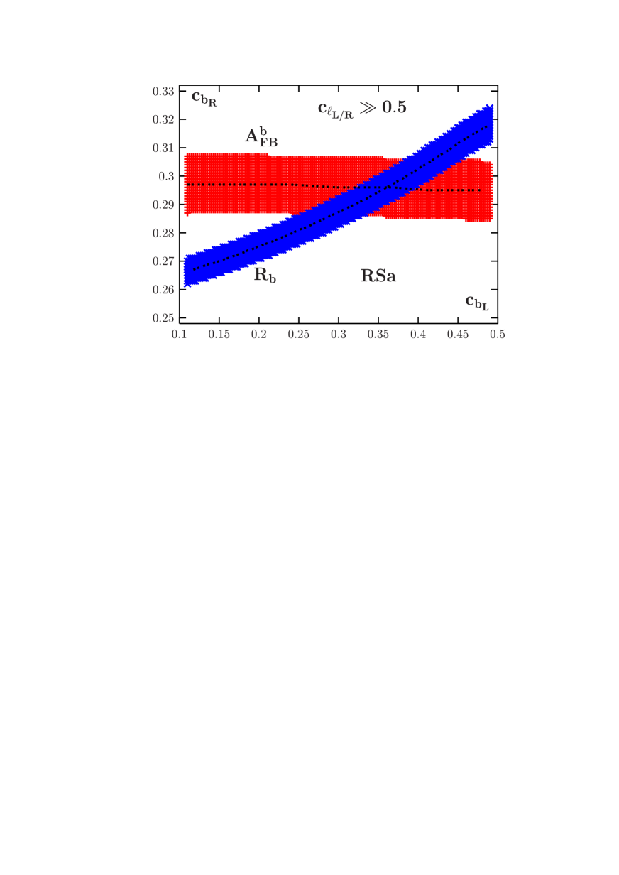
Figure 1: Contour plots in the plane $[c_{b_{L}},c_{b_{R}}]$ for $M_{KK}=3$ TeV and $\sin\theta^{\prime}=0.1$, for which $A_{FB}^{b}$ and $R_{b}$ in the scenario RSa are equal to their experimental values (dotted lines) and are within their $\pm 1\sigma$ bands; $c_{\rm light}\gg 0.5$ for leptons and light quarks.

For heavier KK excitations $M_{KK}>3$ TeV and fixed $\sin\theta^{\prime}$, lower $c_{b_{R}}$ and $c_{b_{L}}$ values are required to increase $|F(c)|$ and thus to compensate the $1/M_{KK}^{2}$ decrease of $|\Delta Q_{Z}^{b_{L,R}}/Q_{Z}^{b_{L,R}}|$, eq. (4). Alternatively, for $\sin\theta^{\prime}$ larger than 0.1, lower $c(b_{R})$ values which compensate the decrease of the $g_{Z^{\prime}}$ effect in $\Delta Q_{Z}^{b_{R}}/Q_{Z}^{b_{R}}$ are required [the $g_{Z^{\prime}}$ coupling is annihilated by the charge $Q_{Z^{\prime}}^{b_{L}}$ in $\Delta Q_{Z}^{b_{L}}/Q_{Z}^{b_{L}}$].

Thus, it is remarkable that both the measurements of $A_{FB}^{b}$ and $R_{b}$ can be reproduced for $c_{b_{L/R}}$ values of order unity, which means that no additional scale is introduced in the model as explained in section 2.1. Given the above discussion on $c$ parameters, the favored values for $M_{KK}$ and $\sin\theta^{\prime}$ (the $kR_{c}$ influence being weak), with regard to a realistic heavy quark mass spectrum, are those chosen for Fig. 1. For the optimal $c$ values, $c_{b_{L}}=0.47$ and $c_{b_{R}}=0.305$ which reproduce the experimental values of $A_{FB}^{b}$ and $R_{b}$ [as noted earlier, the value $c_{t_{R}}=-0.5$ can be chosen as to maximize $m_{t}$, while $c_{t_{L}}=c_{b_{L}}$], the approximate $m_{t}$ and $m_{b}$ values which can be obtained via the geometrical mechanism discussed in section 2, are such that $m_{b}\sim 40$ GeV and $m_{t}\sim 75$ GeV. Both of these generated masses are far from the experimentally measured values. However, these differences can easily originate from the full three–flavor mixing effects, significant contribution from the mixing with the first KK excitations as discussed in Ref. [31] in the case of the top quark, or from a reasonably small hierarchy among the five–dimensional Yukawa couplings. Indeed, the quark mass values given above correspond to a theory in which the Higgs boson is exactly confined on the TeV-brane with the natural choice $Y^{(5)}=\kappa/\sqrt{k}$, where $\kappa$ (relating the five–dimensional Yukawa coupling to the parameter $k$ as usual [20, 31, 21]) taken equal to unity. The actual top and bottom masses are reproduced for $\kappa_{t}\sim 2$ and $\kappa_{b}\sim 0.1$; such $\kappa$ values are acceptable as they correspond to almost universal $Y^{(5)}$ couplings and introduce mass parameters of an order of magnitude relatively close to the fundamental energy scale $k$.

Finally, let us make a few remarks on the case of leptons $\ell=e,\mu$ and $\tau$. The constraints from LEP1 and SLC measurements are very tight since the decay widths $\Gamma_{\ell}$ and the asymmetries $A_{\ell}$ and, in particular the measurement of $A_{e}$ from the left–right asymmetry and $A_{\tau}$ in polarized $\tau$ decays, are determined at the percent level. However, it is known that $A_{e}$, which is the most precisely measured quantity, shows a $\sim 1.7$ standard deviation with respect to the prediction in the SM, $A_{e}^{\rm SLD}=0.1516\pm 0.0021$ compared to the fitted value $A_{e}^{\rm SM}=0.1480$ [the deviation drops slightly in $A_{\ell}$ when all leptonic asymmetries are averaged and lepton–universality is assumed]. It is tempting to try to explain this discrepancy within the RS framework with the extended gauge structure. To do so, one can choose a value $c_{e_{R}}\sim 0.56$ [in agreement with the analysis of Ref. [23] of oblique $S$ and $T$ parameters] while the value of $c_{e_{L}}$ can be taken to be much larger, $c_{e_{L}}\gg 0.5$. Again for $M_{KK}=3$ TeV and $\sin\theta^{\prime}=0.1$, one obtains then for the electron asymmetry $A_{e}=0.1504$, which is only $-0.5\sigma$ away from the measured value by SLD. This choice of parameters will also generate an additional deviation in $A_{FB}^{b}\equiv\frac{3}{4}A_{e}A_{b}$; still, there is a choice of $c$ parameters in the $b$ quark sector which keeps the FB asymmetry close to its measured value. Thus, a judicious choice of the $c$ parameters in both the bottom quark and electron sectors can allow to relax the tension between the two measurements which provide the best individual determinations of the weak mixing angle $\sin^{2}\theta_{W}$ and, thus, provide a very nice global fit to the precision data.

3.3 The FB asymmetry in scenario RSb

In the second scenario RSb, where only the $I_{3R}$ values and thus the $Q_{X}$ charges for the down–type right–handed quarks are modified with respect to the previous scenario in which $Q_{X}=\frac{1}{2}(B-L)$, the contributions of the KK excitations to the $Zb\bar{b}$ coupling are

$$\frac{\Delta Q_{Z}^{b_{L}}}{Q_{Z}^{b_{L}}}\simeq\frac{M_{Z}^{2}}{(0.4M_{KK})^{2}}\bigg{[}1+\frac{1}{4F(c_{b_{L}})}-0.09\bigg{]}F(c_{b_{L}})\,,$$ (20)

$$\frac{\Delta Q_{Z}^{b_{R}}}{Q_{Z}^{b_{R}}}\simeq\frac{M_{Z}^{2}}{(0.4M_{KK})^{2}}\bigg{[}1+\frac{1}{4F(c_{b_{R}})}-\frac{1.5}{\sin^{2}\theta^{\prime}}\bigg{]}F(c_{b_{R}})$$ (21)

where we have used again the approximation $\sin^{2}\theta^{\prime}\ll 1$. The effect of the isospin choice $I_{3R}^{b_{R}}=+\frac{1}{2}$ will be simply to reverse the sign of the contribution proportional to $\sin^{-2}\theta^{\prime}$ in the charge $Q_{Z}^{b_{R}}$ and, therefore, one can have contributions $\Delta Q_{Z}^{b_{L}}/Q_{Z}^{b_{L}}<0$ and $\Delta Q_{Z}^{b_{R}}/Q_{Z}^{b_{R}}>0$ without flipping the sign of the charge $Q_{Z}^{b_{R}}$ in contrast to the previous situation. One can then cure the $A_{FB}^{b}(M_{Z})$ anomaly and simultaneously leave $R_{b}$ almost unchanged, eq. (16), without too large corrections for the $b_{R}$ coupling to the $Z$ boson.

In Fig. 2, assuming $M_{KK}=3$ TeV (in order to address the gauge hierarchy problem) and $\sin\theta^{\prime}=0.1$ and using $c_{\rm light}\gg 0.5$ in such a way that the observables involving leptons and light quarks are not affected, we show in the $[c_{b_{L}},c_{b_{R}}]$ plane the predicted values of $A_{FB}^{b}(M_{Z})$ and $R_{b}$ in this second scenario (the dotted lines); the bands represent the two observables when the $1\sigma$ experimental errors are included. One can see that, as previously, there is a set of $[c_{b_{L}},c_{b_{R}}]$ assignments for which the experimental values of $A_{FB}^{b}$ and $R_{b}$ are reproduced. However, here, one needs values of $c_{b_{R}}$ very close to $0.5$ to resolve the $A_{FB}^{b}(M_{Z})$ anomaly. Note also that, exactly as in scenario RSa, with a judicious choice of $c$ parameters for the electron, one can also explain the slight discrepancy of $A_{e}$ with the value measured at SLD.

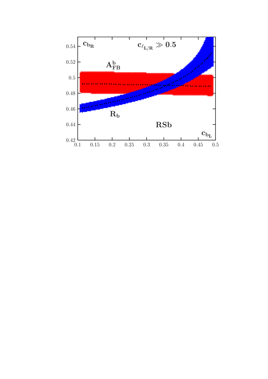
Figure 2: Contour plots in the plane $[c_{b_{L}},c_{b_{R}}]$ for $M_{KK}=3$ TeV and $\sin\theta^{\prime}=0.1$, for which $A_{FB}^{b}$ and $R_{b}$ in the scenario RSb are equal to their experimental values (dotted lines) and are within their $\pm 1\sigma$ bands; $c_{\rm light}\gg 0.5$ for leptons and light quarks.

4. $\mathbf{A_{FB}^{b}}$ outside the Z-pole

To derive the FB asymmetry [and the production cross section] of the bottom quarks outside the Z–pole, one has to take into account the usual $s$–channel virtual photon and $Z$ boson exchanges but also, in principle, the exchange of the heavy $KK$ states $V^{(1)}\equiv\gamma^{(1)},Z^{(1)},Z^{\prime(1)}$ as well as their interference terms. At the tree level, the differential cross for the production of a fermion pair in $e^{+}e^{-}$ collisions, $e^{+}e^{-}\to f\bar{f}$, can be written as

$$\frac{{\rm d}\sigma_{f}}{{\rm d}\cos\theta}=\frac{3}{8}\ \sigma_{0}\ N_{c}\beta_{f}\left[(1+\beta_{f}^{2}\cos^{2}\theta)Q_{1}+(1-\beta^{2}_{f})Q_{2}+2\beta_{f}\cos\theta Q_{3}\right]$$ (22)

with $\beta_{f}=(1-4m_{f}^{2}/s)^{1/2}$ the velocity of the final state fermion, $\theta$ specifying its direction with respect to the incoming electron and $N_{c}$ its color factor and where $\sigma_{0}=4\pi\alpha^{2}/3s$ is the point–like QED cross section for muon pair production. Integrating over the scatting angle, the total production cross section $\sigma_{f}(s)$ and the FB asymmetry $A_{FB}^{f}(s)$ are then given by

$$\sigma_{f}= \frac{3}{4}\sigma_{0}N_{c}\beta_{f}\left[(1+\frac{1}{3}\beta_{f}^{2})Q_{1}+(1-\beta_{f}^{2})Q_{2}\right]\;\; \stackrel{{\scriptstyle\sqrt{s}\gg m_{f}}}{{\longrightarrow}}\;\;N_{c}\sigma_{0}Q_{1}$$ (23)

$$A_{FB}^{f}= \beta_{f}Q_{3}\left[(1+\frac{1}{3}\beta_{f}^{2})Q_{1}+(1-\beta_{f}^{2})Q_{2}\right]^{-1}\;\; \stackrel{{\scriptstyle\sqrt{s}\gg m_{f}}}{{\longrightarrow}}\;\;\frac{3}{4}\frac{Q_{3}}{Q_{1}}$$ (24)

In terms of the helicity amplitudes $Q_{ij}$ with $i,j=L,R$, the charges $Q_{1,2,3}$ are given by [32]

$$Q_{1} = \frac{1}{4}\left[\;|Q_{LL}|^{2}+|Q_{RR}|^{2}+|Q_{RL}|^{2}+|Q_{LR}|^{2}\right]$$

$$Q_{2} = \frac{1}{2}{\rm Re}\ \left[\;Q_{LL}Q_{RL}^{*}+Q_{RR}Q_{LR}^{*}\right]$$

$$Q_{3} = \frac{1}{4}\left[\;|Q_{LL}|^{2}+|Q_{RR}|^{2}-|Q_{RL}|^{2}-|Q_{LR}|^{2}\right]$$ (25)

Taking into account all exchanged gauge bosons, the helicity amplitudes $Q_{ij}$ read

$$Q_{ij}=Q^{e}_{\gamma}Q^{f}_{\gamma}+\frac{Q_{Z}^{e_{i}}Q_{Z}^{f_{j}}}{s_{W}^{2}c_{W}^{2}}\frac{s}{s-M_{Z}^{2}+i\Gamma_{Z}M_{Z}}+\sum_{V}\frac{g_{V}^{2}}{e^{2}}Q_{V}^{e_{i}}Q_{V}^{f_{j}}Q_{V}(c_{e_{i}})Q_{V}(c_{f_{j}})\frac{s}{s-M_{V}^{2}}$$ (26)

where $g_{V}=e,g_{Z}=e/s_{W}c_{W},g_{Z^{\prime}}$ for $V=\gamma^{(1)},Z^{(1)},Z^{\prime(1)}$, $Q_{\gamma^{(1)},Z^{(1)}}=Q(c)$ and $Q_{Z^{\prime(1)}}=Q^{\prime}(c)$.

To evaluate the FB asymmetry for $b$–quarks just below or above the $Z$ resonance, $\sqrt{s}\sim M_{Z}$, one can safely neglect the contributions of the KK excitations that are exchanged in the $s$–channel since these states are relatively heavy, $M_{KK}\gtrsim 3$ TeV, and their couplings to the initial state electrons are rather small. In fact, even at LEP2 energies, $\sqrt{s}\sim 200$ GeV, the effects of the exchanged heavy excitations can be also neglected as the experimental errors in the measurement of $A_{FB}^{b}(s)$ are rather large [8]. One then needs to consider solely the photon and the $Z$ boson exchange contributions and include the mixing effect of the $Z$ boson with the gauge boson KK states as discussed earlier. Note that one has to take into account the mixing between the $B_{0}$ and $\bar{B}_{0}$ mesons when the $b$–quark is tagged through its semi–leptonic decays for instance as is the case at experiments far below the $Z$–pole from PEP to TRISTAN; the bare asymmetry has to be then multiplied by a mixing factor $A_{FB}^{\ell}=(1-2\chi)A_{FB}^{b}$ where the parameter $\chi$ is measured to be $\chi\simeq 0.125$ [2].

In principle, to have a very accurate determination of the asymmetry, some higher order effects [4] need to be included in eq. (22). Besides the $b$–mass effects and the QCD radiative corrections [involving again the $m_{b}$ effects] which can be readily implemented [4, 33], very important effects are the electroweak radiative corrections and, in particular, initial state radiation (ISR) of photons which are crucial especially at energies $\sqrt{s}\raisebox{-3.69899pt}{~{}\shortstack{$>$ \\ [-0.07cm] $\sim$}}~{}M_{Z}$, as it allows for the return to the $Z$–pole where the $e^{+}e^{-}\to b\bar{b}$ rate becomes huge, if no cut is applied on the photon energy. The latter corrections can only be implemented in a Monte–Carlo based approach which involves a full treatment of the kinematics.

At the $Z$–pole, these higher order effects have been implicitly taken into account as we have evaluated small deviations with respect to the SM prediction given in Ref. [3] and in which they are already incorporated. A few GeV above and below the $Z$ pole, where high precision measurements have also been performed by the LEP experiments [3], this approximation might also hold, except for initial state radiation which needs to be explicitly implemented. We have evaluated the FB asymmetry for $b$-quarks at the three LEP1 running energies $\sqrt{s}=89.55,\,91.26$ and 92.94 GeV in the SM and in the two scenarios RSa and RSb, including the $Z$ and photon exchange and their interference as well as ${\cal O}(\alpha)$ initial state radiation. A constant fudge factor close to unity allows to reproduce exactly the SM curves given in Ref. [3], with the Higgs boson mass taken to be $M_{H}=100$ GeV. Assuming the same fudge factor, the variation of $A_{FB}^{b}$ with the c.m. energy around the $Z$ pole in the two scenarios RSa [with $c_{b_{L}}=0.37,c_{b_{R}}=0.287$ and $c_{\rm light}\gg 0.5$] and RSb [with $c_{b_{L}}=0.36,c_{b_{R}}=0.49$ and $c_{\rm light}\gg 0.5$] which reproduce as closely as possible the experimental values of $A_{FB}^{b}(s)$ and $R_{b}$ (the fit depends only mildly on $M_{KK}$ and $\sin\theta^{\prime}$), is shown in the left–hand side of Fig. 3 and is compared to the one in the SM; see also Tab. 1. For these sets of parameters corresponding to the best global fit, we find: $R_{b}=0.21618$, $\Delta Q_{Z}^{b_{L}}/Q_{Z}^{b_{L}}=-0.79\%$, $\Delta Q_{Z}^{b_{R}}/Q_{Z}^{b_{R}}=-227\%$ [RSa] and $R_{b}=0.21629$, $\Delta Q_{Z}^{b_{L}}/Q_{Z}^{b_{L}}=-0.85\%$, $\Delta Q_{Z}^{b_{R}}/Q_{Z}^{b_{R}}=+27\%$ [RSb].

For $\sqrt{s}=91.26$ GeV, i.e. very close to the $Z$ pole, the experimental value for $A_{FB}^{b}(s)$ lies almost on top of the predictions in the two RS scenarios. The measurement of the asymmetry at $\sqrt{s}=89.55$ GeV is also perfectly reproduced in the RSb scenario, contrary to the SM case in which the prediction is about $1.2\sigma$ away and to RSa for which there is a large deviation, $2.8\sigma$. In turn, the point at $\sqrt{s}=92.94$ GeV is perfectly reproduced only in the RSa scenario: the prediction in the SM is $2.7\sigma$ away, while in the scenario RSb, the deviation from the experimental central value is at $+2\sigma$ level which is acceptable, though. If one adds the three measurements around the $Z$ pole, the $\chi^{2}$ is much better in the RSb model, $\chi^{2}_{\rm RSb}\simeq 4.2$, than in the SM, $\chi^{2}_{\rm SM}\simeq 15.3$. In the scenario RSa, the $\chi^{2}$ is better than in the SM, $\chi^{2}_{\rm RSa}\simeq 8.5$, despite of the large deviation at $\sqrt{s}=89.55$ GeV. This is a consequence of the fact that the point at $\sqrt{s}\simeq M_{Z}$ has a much larger weight in the averaging procedure as its corresponding experimental error is much smaller.

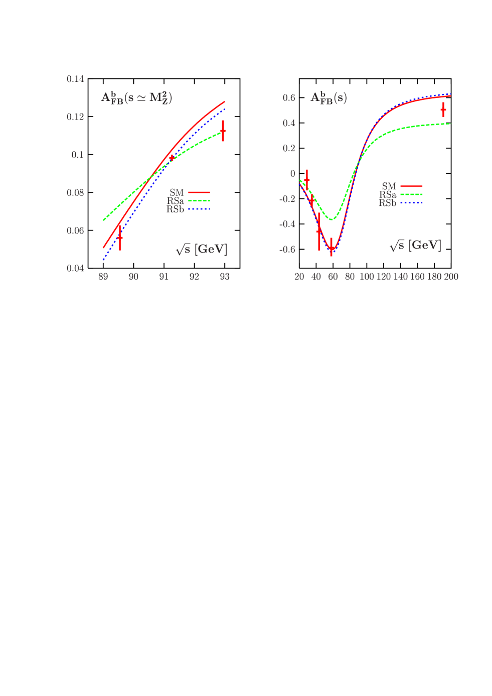
Figure 3: The FB asymmetry $A_{FB}^{b}$ at LEP1 (left) and outside the $Z$ resonance (right) as a function of the c.m. energy. Shown are the predictions in the SM and in the two RS scenarios RSa [with $c_{b_{L}}=0.37,c_{b_{R}}=0.287,c_{\rm light}\gg 0.5$] and RSb [with $c_{b_{L}}=0.36,c_{b_{R}}=0.49,c_{\rm light}\gg 0.5$] for $M_{KK}=3$ TeV and $\sin\theta^{\prime}=0.1$, as well as the various experimental measurements with their error bars.

$\sqrt{s}$	Experimental value	SM sd	$\chi^{2}$	RSa sd	$\chi^{2}$	RSb sd	$\chi^{2}$
89.55 GeV	$0.0560\pm 0.0066$	$+1.2$		$+2.8$		$+0.4$
91.26 GeV	$0.0982\pm 0.0017$	$+2.5$	$15.3$	$+0.5$	$8.5$	$-0.1$	$4.2$
92.94 GeV	$0.1125\pm 0.0055$	$+2.7$		$+0.4$		$+2.0$
29 GeV	$-0.052\pm 0.081$	$-1.5$		$-0.8$		$-1.6$
35 GeV	$-0.214\pm 0.050$	$-1.0$		$+0.9$		$-1.2$
44 GeV	$-0.460\pm 0.147$	$+0.3$	$7.6$	$+1.3$	$14$	$+0.1$	$9.8$
58 GeV	$-0.588\pm 0.078$	$-0.2$		$+2.7$		$-0.4$
190.7 GeV	$0.5055\pm 0.058$	$+2.0$		$-1.9$		$+2.3$

Table 1: The asymmetry $A_{FB}^{b}(s)$ [corrected for $B$ meson mixing] as measured at various c.m. energies, and the standard deviations in the SM and in the two scenarios RSa and RSb. The measured values and the errors at LEP energies are from Refs. [3, 8] and at lower energies, they are taken from the summary given in Ref. [6].

Let us now turn to energies far below [from PEP to TRISTAN] and far above [LEP2] the $Z$–pole for which the experimental values of $A_{FB}^{b}$ with the error bars are given, respectively, in Refs. [5, 7] and Ref. [8]; these values are summarized in the lower part of Tab. 1. We have calculated the asymmetry $A_{FB}^{b}(s)$ as a function of the c.m. energy, taking into account only the effects of $B_{0}$–$\bar{B}_{0}$ mixing. The results for the FB asymmetry in the SM and the two RS scenarios are shown in the right–hand side of Fig. 3 and are compared to the experimental values with the error bars that are given in Table 1.

Here, although the experimental errors are rather large, the general trend is clearly that the predictions for $A_{FB}^{b}(s)$ in the RSb scenario as well as in the SM [which are almost identical] are closer to the measured values. There are large deviations between the predictions in scenario RSa and the experimental values, in particular at the energy $\sqrt{s}=58$ GeV, where the difference is at the level of $2.7\sigma$. Adding all the measurements outside the $Z$–pole region, the $\chi^{2}$ in the SM and in the RSb scenarios, $\chi^{2}_{\rm SM}\simeq 7.6$ and $\chi^{2}_{\rm RSb}\simeq 9.8$, are much better than in the RSa scenario, $\chi^{2}_{\rm RSa}\simeq 14$.

In total, when all measurements around and off the $Z$ pole are considered and if the measurement of $R_{b}$ is included, the agreement between the theoretical prediction and the experimental data is excellent in the RSb model where the overall $\chi^{2}$ is $\chi^{2}_{\rm RSb}\simeq 14$, which corresponds to a probability of a few percent. In contrast, the prediction in scenario RSa is not satisfactory as $\chi^{2}_{\rm RSa}\simeq 22.5$ (which corresponds to a probability that is one order of magnitude worse than in RSb) is as bad as in the SM, $\chi^{2}_{\rm SM}\simeq 23.4$. Thus, one can conclude that only in scenario RSb the $A_{FB}^{b}$ anomaly is resolved both at the $Z$–pole and outside the pole. We should however stress again that, while our results for $A_{FB}^{b}$ on the $Z$–pole, and to a lesser extent a few GeV around the pole, are quite robust as we analyzed small deviations compared to the SM values which include all refinements and higher order effects, the results off the $Z$–pole are less accurate. A full Monte-Carlo analysis, including eventually the experimental cuts [in particular for ISR] is required to make very precise statements.

Before closing this section, let us make a brief comment on a scenario proposed in Ref. [14] where, in addition to the possible modification of the ${\rm SU(2)_{R}}$ assignment of the $b_{R}$ quarks as in our scenario RSb, the assignments for the left–handed quarks are also changed, and one has the representation $Q_{L}^{i}\equiv({\bf 2},{\bf 2})_{2/3}$. In this case, the two multiplet embeddings for the isospin up–type $u_{R}^{i}$ quarks allowing invariant Yukawa couplings are: $u_{R}^{i}\in({\bf 1},{\bf 1})_{2/3}$ or $({\bf 1},{\bf 3})_{2/3}\oplus({\bf 3},{\bf 1})_{2/3}$. In this context, the necessary shift in the $Z\bar{b}_{R}b_{R}$ coupling ($\Delta Q_{Z}^{b_{R}}/Q_{Z}^{b_{R}}>0$) that could explain the $A_{FB}^{b}$ anomaly at the $Z$ pole can be achieved, assuming that the smallness of the ratio $m_{b}/m_{t}$ comes from a strong hierarchy among coupling constants [14]. However, we find that the best fit of $A_{FB}^{b}(s)$ and $R_{b}$ corresponds to $\chi^{2}\simeq 19.4$ which improves the SM case, but is not as good as our scenario RSb. This fit is obtained for $c_{b_{R}}=0.525$ implying $\Delta Q_{Z}^{b_{R}}/Q_{Z}^{b_{R}}=+8.5\%$ if $M_{KK}=3$ TeV and $\sin\theta^{\prime}\!=\!0.1$, the dependence on $M_{KK}$ and $\sin\theta^{\prime}$ being small once again. The reason for this degradation of the fit is that in order to reproduce simultaneously $R_{b}$ and $A_{FB}^{b}(s)$, one should have a correction $|\Delta Q_{Z}^{b_{L}}/Q_{Z}^{b_{L}}|$ of order of the percent [c.f. eq. (16)] while in this case, in contrast, the bidoublet nature of $b_{L}$ forces this correction to vanish. The breaking due to the boundary conditions makes this vanishing imperfect but these effects lead typically to too small deviations: $|\Delta Q_{Z}^{b_{L}}/Q_{Z}^{b_{L}}|<10^{-3}$ [16].

5. Expectations for the ILC

In this section, we analyze the prospects for observing the effects of the new KK states predicted in the RS scenarios discussed here at the ILC, as it is a straightforward generalization of what has been discussed in the previous sections. At the hadron colliders Tevatron and LHC, the situation is more delicate and the search will be more complicated as the main decay modes of the KK states [contrary to conventional $Z^{\prime}$ bosons from GUTs for which BR$(Z^{\prime}\to e^{+}e^{-},\mu^{+}\mu^{-})$ is at the level of a few percent] will be into top and bottom quark pairs which have large QCD backgrounds; see for instance the general analyses performed in Ref. [34]. A detailed account of the expectations at these these colliders in the particular model discussion here will be given in Ref. [35].

5.1 Expectations for bottom quarks

At the GigaZ option of the ILC, i.e. when running the collider at c.m. energies close to the $Z$–pole, the LEP1 and SLC precision measurements discussed previously can be vastly improved, as the planed luminosity will be much higher and the longitudinal polarization of the initial beams available. This will allow to have a more significant determination of the $Zb\bar{b}$ vertex and thus, to probe the mixing between the $Z$ boson and the KK states with a much higher accuracy. The accuracies for determining $R_{b}$ and, using the polarization asymmetry $A_{e}$ from $A_{LR}$ and $A_{b}$ from $A_{LR,FB}^{b}$ by simply extrapolating the results from LEP1 and SLC are shown in Table 2. For the normalized partial width $R_{b}$, we assume that the double $b$–tag method will be applied as for LEP1 but that, for a given purity, the $b$–jet tagging efficiency will be multiplied by a factor of three as can be inferred from SLD. For $A_{b}$, we use the effective efficiency from SLD multiplied by a factor of two given the improved algorithms already foreseen and the better angular coverage of the micro–vertex detector at the ILC. Finally, for $A_{e}$, we have assumed that the dominant systematical error from SLD, beam polarization, will be removed by using positron polarization.

In view of the very high sensitivity of GigaZ, one can stand a reduction of the new effects predicted in the RS scenario by up to two orders of magnitude. This would allow to set an upper limit on the KK mass in the 15–30 TeV range. As pointed out already in Ref. [36], GigaZ through high precision measurements, can therefore already fully cover the RS scenario in a range of parameters which does not reintroduce fine–tuning. It can confirm without ambiguity the indication observed on $A_{e}$ at SLD and establish at a very sensitive level that light fermions are weakly affected, ruling out alternative interpretations [note that in Little Higgs and Technicolor models, for instance, there would be no large effects in the $b$–quark sector anyway]. The measurement of $A_{e}$ gives the electron coupling to the $Z^{\prime}$ boson and, therefore, allows to estimate the interference term at higher c.m. energy between the $Z$ and photon exchanges and the KK excitations.

Energy	Observables	Error %	Deviation %
GigaZ	$R_{\rm b}$	0.015	0.3$\pm$0.3
	$A_{\rm b}$	0.03	–3.9$\pm$1.4
	$A_{\rm e}$	0.01	2.4$\pm$1.4
500 GeV	$A_{\rm LR}$	0.3	+32

Table 2: Deviations and accuracies expected at GigaZ in the $b$ and electron sectors assuming the full accuracy provided by polarized electrons and positrons. For ILC operating at $\sqrt{s}=500$ GeV, one assumes a luminosity of 500 fb^-1 with polarized electrons.

At higher energies, using the formulae derived in section 4 and assuming $c(e_{R})=0.56$, one can easily predict the signals which can be observed at ILC. For the $b$–tagging efficiency/purity at $\sqrt{s}=500$ GeV, we have assumed the same efficiency for double tagging. In addition to the selection effect, one should worry about the determination of the integrated luminosity and, for some part of the analysis, the knowledge of the beam polarization. For the luminosity, ILC intends to achieve the 10^-4 level, which is sufficient to fulfill our goals. For the polarization, one can use the $e^{+}e^{-}\to W^{+}W^{-}$ channel which has a strong polarization asymmetry, as a very effective and realistic analyzer of electron polarization. Given the huge cross section of the process, there is no limitation coming from statistics.

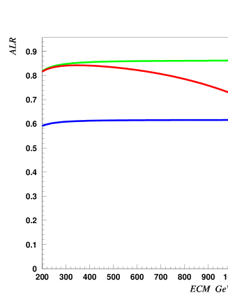
Figure 4: Energy dependence of the Left–Right polarization asymmetry for $b$–quarks in the SM and the RSa (left) and RSb (right) case including the KK contributions and in the pure mixing case. The blue curve is for the SM, the green curve corresponds to mixing only while the red curve takes into account KK exchange.

The lower part of Table 2 shows the accuracy of the $A_{LR}$ measurement with ${\cal L}=500$ fb^-1; it is lower than at GigaZ but the effect is much larger as one can already notice at LEP2 energy from Fig. 4. The study of the energy dependence of appropriate observables will allow to estimate the masses of the KK excitations. This is shown in Fig. 4 for the RSa case where one sees a clear difference between a pure mixing effect [the flat green curve] which dominates a low energies and the contribution of the KK states [the red curve which contains both contributions] which has an energy slope which allows to estimate the KK mass. If one uses the high energy data alone, without any theoretical input and without using the measurement of the mixing effect dominant at low energy, the error on the KK mass would be at the 10% level for a 3 TeV KK state. One can perform much better by noting that the mixing effect is proportional to $F(c_{q_{R}})/(\sin\theta^{\prime}M_{KK})^{2}$. For the heavy top quark, one can assume that $F(c_{t_{R}})$ is close to the asymptotic value, $\sim-8$, so that the mixing determines the denominator. This allows to extract the $c_{f_{R}}$ values for the electron and the $b$ quarks and thus the $Z^{\prime}$ couplings; in this case one can estimate $M_{KK}$ to about a percent. This argument indicates how ILC could allow to extract precisely the various parameters of the RS model.

5.2 Expectations for top quarks

Excellent statistical accuracies are expected for the channel $e^{+}e^{-}\to t\bar{t}$ since $\sim 4\times 10^{5}$ events can be collected with ${\cal L}=500$ fb^-1 at $\sqrt{s}=500$ GeV. A key issue will be the signal/background ratio which drives systematic errors of the measurements. Since top quark pairs are mostly made of six–jet events or four–jet events with one isolated lepton, with two of these jets being $b$ quarks, they can be very well separated from background events by using the following observations: $i)$ $W^{+}W^{-}$ events which do not contain $b$–jets, have 4 jets and are very forward peaked; $ii)$ $ZZ$ events are an order of magnitude less numerous, have 4 jets and are forward peaked; $iii)$ $b\bar{b}$ pairs with multi gluons give an incompressible but small background; $iv)$ $ZW^{+}W^{-}$ events are an order of magnitude below the signal at 500 GeV; the channel $Z\to b\bar{b}$ can fake the signal topology but is at the % level only.

One can thus clearly tag the latter background and eliminate it further by reconstructing the $Z$ boson mass using the resolution anticipated with particle flow methods developed for ILC detectors which should lead to a few percent resolution on the $Z$ boson mass. This method will also allow to reconstruct the $W$ boson mass which will further reduce the 4 jet QCD background. Note also that selecting isolated leptons would decrease the efficiency by a factor of two but allows for a $\sim 100\%$ purity. Therefore, one can conclude that the statistical accuracy achievable at the ILC is unlikely to be jeopardized by an insufficient knowledge of the background contamination or of the signal efficiency. This, however, needs confirmation with appropriate simulation and reconstruction tools.

Energy	Observables	Error %	Deviation %
500 GeV	$R_{\rm t}$	0.2	+24
	$A_{\rm LR}$	0.1	+200

Table 3: Deviations and accuracies expected at ILC in the top sector assuming $\sqrt{s}=500$ GeV and ${\cal L}=500$ fb^-1 and electron polarization.

Table 3 displays the expected accuracies in the measurement of $R_{t}$ and $A_{LR}^{t}$ with $\sqrt{s}=500$ GeV and ${\cal L}=500$ fb^-1, with longitudinally polarized beams. Taking as an example the LR asymmetry, the energy dependence of which is shown in Fig. 5, a huge deviation is expected from the SM case, if one assumes $c(t_{R})=-0.5$ as previously discussed. This means that given the accuracies expected at the ILC, one could as for GigaZ, allow for two orders magnitude reduction in the KK effect and still clearly observe a significant deviation. Thus, in the top quark sector, the sensitivity of the ILC is also sufficient to exclude or confirm the RS scenario; see also Ref. [37] for instance.

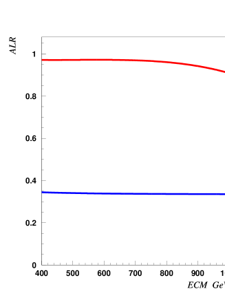
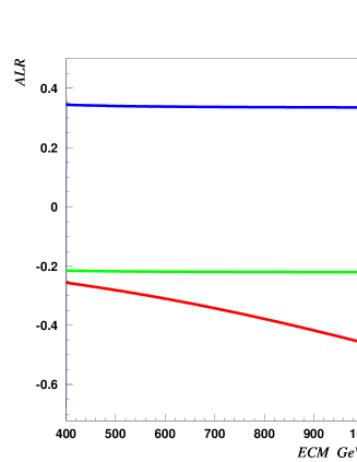
Figure 5: Energy dependence of the Left–Right polarization asymmetry for top quarks in the SM and in the RSa and RSb scenarios. Conventions are as in the previous figure.

5. Conclusion

In this paper, we have analyzed the impact of a RS extra dimensional model with the extended ${\rm SU(2)_{L}\times SU(2)_{R}\times U(1)_{X}}$ gauge structure allowing relatively light KK excitations, on the high precision electroweak data. In this model, in order to interpret the mass hierarchies, the fermions are localized differently along the extra dimension so that the electroweak interactions for the heavy third generation fermions are naturally different from those of light fermions. The mixing between the $Z$ boson with its KK excitations and those of the new $Z^{\prime}$ boson, is then large enough to significantly affect the $Zb\bar{b}$ vertex, while keeping the $Z$ coupling to light fermions almost unchanged. We have shown that with a judicious choice of the parameter assignments in the $b$–quark sector and for order TeV KK states, so that the gauge hierarchy problem is addressed, the $\sim 3\sigma$ discrepancy of the forward–backward asymmetry of $b$–quark jets, $A_{FB}^{b}$, with measurements performed on the $Z$–pole can be resolved, while all other precision electroweak data including the normalized $Z\to b\bar{b}$ partial decay width $R_{b}$, stay almost unaffected.

The key point of the analysis is to generate a rather large contribution to the right–handed $Zb_{R}\bar{b}_{R}$ charge which is small in the SM, to provide the required negative shift in $A_{FB}^{b}$; this contribution is annihilated by a relatively smaller contribution to the left–handed $Zb_{L}\bar{b}_{L}$ charge, leading to an almost constant $R_{b}$ value. In this context, we have analyzed two possible scenarios. In a first scenario, in which the U(1) group is identified with ${\rm U(1)_{B-L}}$, a large contribution to the $Zb_{R}\bar{b}_{R}$ charge is needed as to flip its sign. However, at energies below and above the $Z$ resonance, although the experimental uncertainties are larger than at LEP1, the theoretical predictions for $A_{FB}^{b}(s)$ are in a rather poor agreement with the experimentally measured values. In a second scenario, the charges of the U(1) group have been chosen such that the $b_{R}$ quark has isospin $I_{3R}^{b_{R}}=+\frac{1}{2}$ with respect to the new ${\rm SU(2)_{R}}$ group. In this case, only a $\sim 30\%$ change of the $Zb_{R}\bar{b}_{R}$ charge is needed to resolve the $A_{FB}^{b}$ anomaly. In this scenario, the predictions for the asymmetry outside the $Z$–pole are also in a good agreement with the experimental data.

This scenario can be tested in detail at future high–energy colliders, and in particular at the ILC. At GigaZ, i.e. when running ILC at energies close to the Z–pole, the LEP1 and SLC precision measurements of $A_{FB}^{b},A_{e}$ and $R_{b}$ can be vastly improved, as longitudinal polarization will be available and the planed luminosities will be much higher. With the expected high accuracies, one could allow for two orders magnitude reduction in the new effects and still clearly observe a significant deviation. At high energies, $\sqrt{s}\raisebox{-3.69899pt}{~{}\shortstack{$>$ \\ [-0.07cm] $\sim$}}~{}500$ GeV, measurements in heavy quark production, in particular in the process $e^{+}e^{-}\to t\bar{t}$, will allow to perform precision measurement of the masses of the KK states and their couplings to fermions. For instance, KK masses of the order of 15–30 TeV can be probed and a mass $M_{KK}\sim 3$ TeV can be measured at the percent level. A detailed discussion of the impact of this model at the LHC and ILC will be given in a forthcoming publication [35].

Acknowledgments: Discussions with Christophe Grojean and Ritesh Singh are greatfully acknowledged; G.M. thanks K. Agashe for useful conversations. The work of A.D. and G.M. is supported by the ANR for the project PHYS@COL&COS under the number NT05-1_43598.

References

- [1] S. Glashow, Nucl. Phys. 22 (1961) 579; S. Weinberg, Phys. Rev. Lett. 19 (1967) 1264; A. Salam, in “Elementary Particle Theory”, ed. N. Svartholm, Almqvist and Wiksells, Stockholm (1969) p. 367.
- [2] Particle Data Group, K. Hagiwara et al., Phys. Rev. D66 (2002) 010001 and S. Eidelman et al., Phys. Let. B592 (2004) 1.
- [3] The LEP Collaborations (ALEPH, DELPHI, L3 and OPAL), the LEP Electroweak Working Group and the SLD Heavy Flavour Group, A combination of preliminary Electroweak measurements and constraints on the Standard Model, Phys. Rep. 427 (2006) 257, hep-ex/0509008, http://lepewwg.web.cern.ch/LEPEWWG. We use the updated values given in the talk of C. Parkes at ICHEP 2006, Moscow.
- [4] A. Djouadi, J. Kühn and P.M. Zerwas, Z. Phys. C46 (1990) 411.
- [5] TASSO Collaboration, M. Althoff et al., Phys. Lett. B146 (1984) 443; TPC Collaboration, H. Aihara et al., Phys. Rev. D31 (1985) 2719; JADE Collaboration, E. Elsen et al., Z. Phys. C46 (1990) 349; TOPAZ Collaboration, A. Shimonoka et al., Phys. Lett. B268 (1991) 457 and Y. Inoue et al., Eur. Phys. J. C18 (2000) 213.
- [6] For a review, see: K. Monig, Rept. Prog. Phys.61 (1998) 999.
- [7] D. Choudhury, T.M.P. Tait and C.E.M. Wagner, Phys. Rev. D65 (2002) 053002.
- [8] The LEP Collaborations and the LEP Electroweak Working Group, hep-ex/0511037.
- [9] See for instance, M.S. Chanowitz, Phys. Rev. Lett. 87 (2001) 231802; G. Altarelli and M.W. Grunewald, Phys. Rept. 403-404 (2004) 189; P. Gambino, Int. J. Mod. Phys. A19 (2004) 808; A. Djouadi, hep-ph/0503172, sec. 1.
- [10] M. Boulware and D. Finell, Phys. Rev. D349 (1991) 48; A. Djouadi, G. Girardi, C. Verzegnassi, W. Hollik and F.M. Renard, Nucl. Phys. B349 (1991) 48.
- [11] X.G. He and G. Valencia, Phys. Rev. D66 (2002) 013004; Phys. Rev. D68 (2003) 033011.
- [12] D. Chang, W.F. Chang and E. Ma, Phys. Rev. D61 (2000) 037301; F. del Aguila , M. Perez-Victoria and J. Santiago JHEP 0009 (2000) 011; R.A. Diaz, R. Martinez and F. Ochoa, Phys.Rev. D72 (2005) 035018.
- [13] See for instance: E. Malkawi, T. Tait and C.P. Yuan, Phys. Lett. B385 (1996) 304; R.S. Chivukula, E.H. Simmons, Phys. Rev. D66 (2002) 015006.
- [14] K. Agashe, R. Contino, L. Da Rold and A. Pomarol, Phys. Lett. B641 (2006) 62.
- [15] G. Cacciapaglia, C. Csaki, G. Marandella and J. Terning, hep-ph/0607146.
- [16] M. Carena, E. Ponton, J. Santiago and C.E.M. Wagner, hep-ph/0607106.
- [17] L. Randall and R. Sundrum, Phys. Rev. Lett. 83 (1999) 3370; M. Gogberashvili, Int. J. Mod. Phys. D11 (2002) 1635.
- [18] A. Pomarol, Phys. Rev. Lett. 85 (2000) 4004; L. Randall and M.D. Schwartz, JHEP 0111 (2001) 003; Phys. Rev. Lett. 88 (2002) 081801; W.D. Goldberger and I.Z. Rothstein, Phys. Rev. D68 (2003) 125011; K. Choi and I.W. Kim, Phys. Rev. D67 (2003) 045005; K. Agashe, A. Delgado and R. Sundrum, Annals Phys. 304 (2003) 145.
- [19] K. Agashe and G. Servant, Phys. Rev. Lett. 93 (2004) 231805; JCAP 0502 (2005) 002.
- [20] T. Gherghetta and A. Pomarol, Nucl. Phys. B586 (2000) 141.
- [21] S. J. Huber and Q. Shafi, Phys. Lett. B498 (2001) 256; Phys. Lett. B544 (2002) 295; Phys. Lett. B583 (2004) 293; Phys. Lett. B512 (2001) 365; S. J. Huber, Nucl. Phys. B666 (2003) 269; S. Chang et al., Phys. Rev. D73 (2006) 033002; G. Moreau and J. I. Silva-Marcos, JHEP 0601 (2006) 048; JHEP 0603 (2006) 090.
- [22] Y. Grossman and M. Neubert, Phys. Lett. B474 (2000) 361; T. Appelquist et al., Phys. Rev. D65 (2002) 105019; T. Gherghetta, Phys. Rev. Lett. 92 (2004) 161601; G. Moreau, Eur. Phys. J. C40 (2005) 539.
- [23] K. Agashe, A. Delgado, M. J. May and R. Sundrum, JHEP 0308 (2003) 050.
- [24] G. Burdman, Phys. Rev. D66 (2002) 076003; C.S. Kim et al., Phys. Rev. D67 (2003) 015001; J.L. Hewett, F.J. Petriello and T.G. Rizzo, JHEP 0209 (2002) 030; S.J. Huber and Q. Shafi, Phys. Rev. D63 (2001) 045010; S.J. Huber, C.A. Lee and Q. Shafi, Phys. Lett. B531 (2002) 112; C. Csaki et al., Phys. Rev. D66 (2002) 064021.
- [25] F. del Aguila, M. Perez-Victoria and J. Santiago, JHEP 0302 (2003) 051; M. Carena, T.M. P. Tait and C.E.M. Wagner, Acta Phys. Polon. B33 (2002) 2355.
- [26] M. Carena, E. Ponton, T.M.P. Tait and C.E.M. Wagner, Phys. Rev. D67 (2003) 096006; M. Carena et al., Phys. Rev. D68 (2003) 035010; Phys. Rev. D71 (2005) 015010.
- [27] A. Kehagias and K. Tamvakis, Phys. Lett. B504 (2001) 38.
- [28] H. Davoudiasl, J.L. Hewett and T.G. Rizzo, Phys. Rev. D63 (2001) 075004.
- [29] M. Peskin and T. Takeuchi, Phys. Rev. Lett. 65 (1990) 964; ibid. Phys. Rev. D46 (1992) 381. For a similar approach, see: G. Altarelli and R. Barbieri, Phys. Lett. B253 (1991) 161.
- [30] K. Agashe et al., Phys. Rev. Lett. 93 (2004) 201804; K. Agashe et al., Phys. Rev. D71 (2005) 016002; K. Agashe et al., hep-ph/0606021; hep-ph/0606293.
- [31] F. del Aguila et al., Phys. Lett. B492 (2000) 98; D. E. Kaplan and T. M. Tait, JHEP 0111 (2001) 051; F. del Aguila and J. Santiago, Phys. Lett. B493 (2000) 175.
- [32] L.M. Sehgal and P.M. Zerwas, Nucl. Phys. B183 (1981) 417; A. Djouadi, A. Leike, T. Riemann, D. Schaile and C. Verzegnassi, Z. Phys. C56 (1992) 289.
- [33] J. Jerzak, E. Laemann and P. Zerwas, Phys. Rev. D25 (1982) 1218; A. Djouadi, Z. Phys. C39 (1988) 561; A. Arbuzov, D. Bardin and A. Leike, Mod. Phys. Lett. A7 (1992) 2029; A. Djouadi, B. Lampe and P. Zerwas, Z. Phys. C67 (1995) 123; G. Altarelli and B. Lampe, Nucl. Phys. B391 (1993) 3; V. Ravindran and W. van Neerven, Phys. Lett. B445 (1998) 214; S. Catani and M.H. Seymour, JHEP 9907 (1999) 023; W. Bernreuter et al., Nucl. Phys. B750 (2006) 83.
- [34] T.G. Rizzo JHEP 0306 (2003) 021 and hep-ph/0610104; see also: T. Han, G. Valencia and Y. Wang, Phys. Rev. D70 (2004) 034002.
- [35] A. Djouadi, G. Moreau, F. Richard and R. Singh, analysis in progress.
- [36] J.L. Hewett et al., JHEP 0209 (2002) 030.
- [37] E. De Pree and M. Sher, Phys. Rev. D73 (2006) 095006.