Analysis of Y(2175) as a tetraquark state with QCD sum rules

Zhi-Gang Wang 111E-mail,wangzgyiti@yahoo.com.cn.

Department of Physics, North China Electric Power University, Baoding 071003, P. R. China

Abstract

In this article, we take the point of view that $Y(2175)$ be a tetraquark state which consists of color octet constituents, and calculate its mass and decay constant within the framework of the QCD sum rule approach. We release standard criterion in the QCD sum rules approach and take more phenomenological analysis, the value of the mass of $Y(2175)$ is consistent with experimental data; there may be some tetraquark components in the state $Y(2175)$. If we retain standard criterion, larger mass than experimental data can be obtained, the current $J_{\mu}(x)$ can interpolate a tetraquark state with larger mass, or $Y(2175)$ has some components with larger mass. The dominating contribution comes from the perturbative term, which is in contrast to the sum rules with interpolating currents constructed from diquark pairs. The tetraquark states may consist of color octet constituents rather than diquark pairs.

PACS number: 12.38.Aw, 12.38.Qk

Key words: Y(2175), QCD sum rules

1 Introduction

Recently, Babar collaboration observed a resonance with the quantum numbers $J^{PC}=1^{--}$ near the threshold in process $e^{+}e^{-}\to\phi f_{0}(980)$ via initial-state radiation [1]. Breit-Wigner mass is $m_{Y}=(2.175\pm 0.010\pm 0.015)GeV$ and width is narrow $\Gamma_{Y}=(58\pm 16\pm 20)MeV$. The resonance may be interpreted as an $\bar{s}s$ analogue of $Y(4260)$, or as an $\bar{s}s\bar{s}s$ state that decays predominantly to $\phi f_{0}(980)$. In this article, we take the point of view that the state $Y(2175)$ (thereafter we take the notation $Y(2175)$) be a tetraquark state with the quantum numbers $J^{PC}=1^{--}$, and calculate its mass and decay constant in the framework of the QCD sum rules approach [2, 3, 4]. In the QCD sum rules, operator product expansion is used to expand the time-ordered currents into a series of quark and gluon condensates which parameterize long distance properties of the QCD vacuum. Based on current-hadron duality, we can obtain copious information about the hadronic parameters at phenomenological side.

Whether or not there exists a tetraquark configuration $\bar{s}s\bar{s}s$ which can result in baryonium state is of great importance itself, because it provides a new opportunity for a deeper understanding of low energy QCD. We explore this possibility, later experimental data can confirm or reject this assumption. Interactions of one-gluon exchange and direct instantons lead to significant attractions between the quarks in $0^{+}$ channel, $Y(4260)$ can be taken as consist of scalar diquark ($\epsilon_{kij}c^{T}_{i}C\gamma_{5}s_{j}$) pairs in relative $P$-wave [5]. However, two $s$ quarks cannot cluster together to form a scalar diquark, if $Y(2175)$ is the cousin of $Y(4260)$, why they have so different substructures?

Existence of the tetraquark states has not been confirmed with experimental data yet, however, there are evidences for those exotic states. Numerous candidates with the same quantum numbers $J^{PC}=0^{++}$ below $2GeV$ can not be accommodated in one $q\bar{q}$ nonet, some are supposed to be glueballs, molecules and multiquark states [6, 7]. There maybe different dynamics that dominate $0^{++}$ mesons below and above $1GeV$, which results in two scalar nonets below $1.7GeV$. Attractive interactions of one-gluon exchange favor formation of diquarks in color antitriplet $\overline{3}_{c}$, flavor antitriplet $\overline{3}_{f}$ and spin singlet $1_{s}$. Strong attractions between the states $(qq)_{\overline{3}}$ and $(\bar{q}\bar{q})_{3}$ in $S$-wave may result in a nonet manifested below $1GeV$, while the conventional ${}^{3}P_{0}$ $\bar{q}q$ nonet would have masses about $1.2-1.6GeV$. Furthermore, there are enough candidates for ${}^{3}P_{0}$ $\bar{q}q$ nonet mesons, $a_{0}(1450)$, $f_{0}(1370)$, $K^{*}(1430)$, $f_{0}(1500)$ and $f_{0}(1710)$ [6, 7]. If we take scalar diquarks $U^{a}=\epsilon_{abc}d_{b}^{T}(x)C\gamma_{5}s_{c}(x)$, $D^{a}=\epsilon_{abc}u_{b}^{T}(x)C\gamma_{5}s_{c}(x)$ and $S^{a}=\epsilon_{abc}u_{b}^{T}(x)C\gamma_{5}d_{c}(x)$ as basic constituents, the mass formula of $0^{++}$ nonet mesons below $1GeV$ can be naturally explained. Comparing with the traditional ${\bar{q}}q$ nonet mesons, the mass spectrum is inverted. The lightest state is the non-strange isosinglet ($\bar{S}^{a}S^{a}$), the heaviest are the degenerate isosinglet and isovectors with hidden $\bar{s}s$ pairs, while the four strange states lie in between [6, 7]. The mass spectrum of the scalar nonet mesons as tetraquark states below $1GeV$ has been studied with the QCD sum rules approach [8, 9], for more literature on the tetraquark states consist of diquark pairs with the QCD sum rules approach, one can consult e.g. Refs.[10, 11].

The article is arranged as follows: we derive the QCD sum rules for the mass and decay constant of $Y(2175)$ in section 2; in section 3, numerical results and discussions; section 4 is reserved for conclusion.

2 QCD sum rules for the mass of the $Y(2175)$

In the following, we write down the two-point correlation function Πμ​ν​(p2)subscriptΞ πœ‡πœˆsuperscript𝑝2\Pi_{\mu\nu}(p^{2}) in the QCD sum rules approach,

Πμ​ν​(p2)subscriptΞ πœ‡πœˆsuperscript𝑝2\displaystyle\Pi_{\mu\nu}(p^{2}) $\displaystyle=$ $\displaystyle i\int d^{4}xe^{ip\cdot x}\langle 0|T\{J_{\mu}(x)J_{\nu}^{+}(0)\}|0\rangle\,,$ (1)
$\displaystyle J_{\mu}(x)$ $\displaystyle=$ s¯​(x)​γμ​λa​s​(x)​s¯​(x)​λa​s​(x),¯𝑠π‘₯subscriptπ›Ύπœ‡superscriptπœ†π‘Žπ‘ π‘₯¯𝑠π‘₯superscriptπœ†π‘Žπ‘ π‘₯\displaystyle\bar{s}(x)\gamma_{\mu}\lambda^{a}s(x)\bar{s}(x)\lambda^{a}s(x)\,, (2)
$\displaystyle f_{Y}m^{4}_{Y}\epsilon_{\mu}$ $\displaystyle=$ $\displaystyle\langle 0|J_{\mu}(0)|Y\rangle\,.$ (3)

Where $\lambda^{a}$’s are Gell-Mann matrixes for color $SU(3)$ group, $\epsilon_{\mu}$ and $f_{Y}$ stand for the polarization vector and decay constant of $Y(2175)$, respectively. We take color octet operators s¯​(x)​γμ​λa​s​(x)¯𝑠π‘₯subscriptπ›Ύπœ‡superscriptπœ†π‘Žπ‘ π‘₯\bar{s}(x)\gamma_{\mu}\lambda^{a}s(x) and s¯​(x)​λa​s​(x)¯𝑠π‘₯superscriptπœ†π‘Žπ‘ π‘₯\bar{s}(x)\lambda^{a}s(x) as basic constituents in constructing the vector current $J_{\mu}(x)$. Originally, color octet operators s¯​λa​s¯𝑠superscriptπœ†π‘Žπ‘ \bar{s}\lambda^{a}s, $\bar{q}\lambda^{a}q$ , s¯​γ5​λa​s¯𝑠subscript𝛾5superscriptπœ†π‘Žπ‘ \bar{s}\gamma_{5}\lambda^{a}s and $\bar{q}\gamma_{5}\lambda^{a}q$ were used to construct the interpolating currents for the scalar mesons $a_{0}(980)$ and $f_{0}(980)$ as tetraquark states [12]. There are other two vector current operators $J^{A}_{\mu}(x)$ and $J^{B}_{\mu}(x)$ with the same quantum numbers $J^{PC}=1^{--}$ as $Y(2175)$,

$\displaystyle J^{A}_{\mu}(x)$ $\displaystyle=$ s¯​(x)​γμ​s​(x)​s¯​(x)​s​(x),¯𝑠π‘₯subscriptπ›Ύπœ‡π‘ π‘₯¯𝑠π‘₯𝑠π‘₯\displaystyle\bar{s}(x)\gamma_{\mu}s(x)\bar{s}(x)s(x)\,,
$\displaystyle J^{B}_{\mu}(x)$ $\displaystyle=$ $\displaystyle\epsilon^{kij}\epsilon^{kmn}\left\{s^{T}_{i}(x)C\sigma_{\mu\nu}s_{j}(x)\bar{s}_{m}(x)C\gamma^{\nu}\gamma_{5}\bar{s}^{T}_{n}(x)\right.$ (4)
$\displaystyle\left.+\bar{s}_{i}(x)C\sigma_{\mu\nu}\bar{s}^{T}_{j}(x)s^{T}_{m}(x)C\gamma^{\nu}\gamma_{5}s_{n}(x)\right\}\,.$

Where $k$, $i$, $j$, $m$, $n$ are color indexes, $C$ is charge conjunction matrix, $\mu$ and $\nu$ are Lorentz indexes. If we take color singlet operators s¯​(x)​γμ​s​(x)¯𝑠π‘₯subscriptπ›Ύπœ‡π‘ π‘₯\bar{s}(x)\gamma_{\mu}s(x) and $\bar{s}(x)s(x)$ as basic constituents, and choose the current operator $J^{A}_{\mu}(x)$, which can interpolate a tetraquark state, whether compact state or loose deuteron-like $\phi f_{0}(980)$ bound state, it is difficult to separate the contributions of bound state from scattering $\phi f_{0}(980)$ state. In this article, we take $Y(2175)$ as a baryonium state and choose the current $J_{\mu}(x)$, although $J^{A}_{\mu}(x)$ has non-vanishing coupling with $Y(2175)$. In the diquark-antidiquark model [5], $Y(4260)$ is taken as consist of scalar diquark ($\epsilon_{kij}c^{T}_{i}C\gamma_{5}s_{j}$) pairs in relative $P$-wave. One can take $Y(2175)$ as the cousin of $Y(4260)$, decays $Y(4260)\to J/\psi f_{0}(980)$ and $Y(2175)\to\phi f_{0}(980)$ occur with the same mechanism, however, $Y(2175)$ can not be constructed from scalar $ss$ diquark pairs, because two $s$ quarks can not cluster together to form a scalar diquark due to Fermi statistics, we have to resort to the constituents, a tensor diquark and a vector diquark in relative $S$-wave, to construct the interpolating current, if one insist on that the multiquark current operators should be constructed from diquark pairs [8, 10]. It is odd that the cousins have very different substructures, $Y(4260)$ may have structure c¯​γμ​λa​c​s¯​λa​s+s¯​γμ​λa​s​c¯​λa​c¯𝑐subscriptπ›Ύπœ‡superscriptπœ†π‘Žπ‘Β―π‘ superscriptπœ†π‘Žπ‘ Β―π‘ subscriptπ›Ύπœ‡superscriptπœ†π‘Žπ‘ Β―π‘superscriptπœ†π‘Žπ‘\bar{c}\gamma_{\mu}\lambda^{a}c\bar{s}\lambda^{a}s+\bar{s}\gamma_{\mu}\lambda^{a}s\bar{c}\lambda^{a}c.

The correlation function Πμ​ν​(p)subscriptΞ πœ‡πœˆπ‘\Pi_{\mu\nu}(p) can be decomposed as follows:

Πμ​ν​(p)subscriptΞ πœ‡πœˆπ‘\displaystyle\Pi_{\mu\nu}(p) $\displaystyle=$ βˆ’Ξ 1​(p2)​(gΞΌβ€‹Ξ½βˆ’pμ​pΞ½p2)+Ξ 0​(p2)​pμ​pΞ½p2,subscriptΞ 1superscript𝑝2subscriptπ‘”πœ‡πœˆsubscriptπ‘πœ‡subscriptπ‘πœˆsuperscript𝑝2subscriptΞ 0superscript𝑝2subscriptπ‘πœ‡subscriptπ‘πœˆsuperscript𝑝2\displaystyle-\Pi_{1}(p^{2})\left(g_{\mu\nu}-\frac{p_{\mu}p_{\nu}}{p^{2}}\right)+\Pi_{0}(p^{2})\frac{p_{\mu}p_{\nu}}{p^{2}}, (5)

due to Lorentz covariance. The invariant functions Ξ 1subscriptΞ 1\Pi_{1} and Ξ 0subscriptΞ 0\Pi_{0} stand for the contributions from the vector and scalar mesons, respectively. In this article, we choose the tensor structure $g_{\mu\nu}-\frac{p_{\mu}p_{\nu}}{p^{2}}$ to study the mass of the vector meson.

According to basic assumption of current-hadron duality in the QCD sum rules approach [2], we insert a complete series of intermediate states satisfying unitarity principle with the same quantum numbers as the current operator $J_{\mu}(x)$ into the correlation function in Eq.(1) to obtain the hadronic representation. After isolating the pole term of the lowest state $Y(2175)$, we obtain the following result:

Πμ​ν​(p2)subscriptΞ πœ‡πœˆsuperscript𝑝2\displaystyle\Pi_{\mu\nu}(p^{2}) $\displaystyle=$ $\displaystyle i\int d^{4}xe^{ip\cdot x}\langle 0|J_{\mu}(x)\sum_{n,\epsilon_{n}}\int\frac{d^{3}q}{(2\pi)^{3}2E_{n}}|q_{n},\epsilon_{n}\rangle\langle q_{n},\epsilon_{n}|J_{\nu}^{+}(0)|0\rangle\Theta(t)\,,$ (6)
$\displaystyle=$ $\displaystyle-\frac{f_{Y}^{2}m_{Y}^{8}}{m_{Y}^{2}-p^{2}}\left\{g_{\mu\nu}-\frac{p_{\mu}p_{\nu}}{p^{2}}\right\}+\cdots\,,$
Im​Π1​(s)Ο€ImsubscriptΞ 1π‘ πœ‹\displaystyle\frac{\mbox{Im}\Pi_{1}(s)}{\pi} $\displaystyle=$ fY2​mY8+ρQ​C​Dβ€‹Ξ˜β€‹(sβˆ’s0).superscriptsubscriptπ‘“π‘Œ2superscriptsubscriptπ‘šπ‘Œ8subscriptπœŒπ‘„πΆπ·Ξ˜π‘ subscript𝑠0\displaystyle f_{Y}^{2}m_{Y}^{8}+\rho_{QCD}\Theta(s-s_{0})\,. (7)

The intermediate states are saturated by the states $|q_{n},\epsilon_{n}\rangle$ with the same quantum numbers as $Y(2175)$, high resonances (if there are some) $Y_{1}$, $Y_{2}$, $Y_{3}$ $\cdots$ appear consequentially before continuum states (which can be described by the contributions from asymptotic quarks and gluons) set on. If we choose standard criterion that the dominating contribution comes from the pole terms, $Y_{1}$, $Y_{2}$, $\cdots$ should be concluded in besides $Y(2175)$. It is difficult to analyze those terms qualitatively or quantitatively without experimental data. We approximate the hadronic spectral density Ξ 1​(s)subscriptΞ 1𝑠\Pi_{1}(s) with the corresponding one $\rho_{QCD}$ from perturbative QCD above the threshold $s_{0}$. We will revisit this subject in next section.

In the following, we briefly outline operator product expansion for the correlation function Πμ​ν​(p)subscriptΞ πœ‡πœˆπ‘\Pi_{\mu\nu}(p) in perturbative QCD theory. The calculations are performed at large space-like momentum region $p^{2}\ll 0$, which corresponds to small distance $x\approx 0$ required by validity of operator product expansion approach. We write down the ”full” propagator $S_{ab}(x)$ of a massive light quark in the presence of the vacuum condensates firstly [2]222One can consult the last article of Ref.[2] for technical details in deriving the full propagator.,

$\displaystyle S_{ab}(x)$ $\displaystyle=$ i​δa​b​​x2​π2​x4βˆ’Ξ΄a​b​ms4​π2​x2βˆ’Ξ΄a​b12β€‹βŸ¨s¯​s⟩+i​δa​b48​msβ€‹βŸ¨s¯​sβŸ©β€‹β€‹xβˆ’π‘–subscriptπ›Ώπ‘Žπ‘π‘₯2superscriptπœ‹2superscriptπ‘₯4subscriptπ›Ώπ‘Žπ‘subscriptπ‘šπ‘ 4superscriptπœ‹2superscriptπ‘₯2subscriptπ›Ώπ‘Žπ‘12delimited-βŸ¨βŸ©Β―π‘ π‘ limit-from𝑖subscriptπ›Ώπ‘Žπ‘48subscriptπ‘šπ‘ delimited-βŸ¨βŸ©Β―π‘ π‘ π‘₯\displaystyle\frac{i\delta_{ab}\!\not\!{x}}{2\pi^{2}x^{4}}-\frac{\delta_{ab}m_{s}}{4\pi^{2}x^{2}}-\frac{\delta_{ab}}{12}\langle\bar{s}s\rangle+\frac{i\delta_{ab}}{48}m_{s}\langle\bar{s}s\rangle\!\not\!{x}- (8)
Ξ΄a​b​x2192β€‹βŸ¨s¯​gs​σ​G​s⟩+i​δa​b​x21152​msβ€‹βŸ¨s¯​gs​σ​G​sβŸ©β€‹β€‹xβˆ’subscriptπ›Ώπ‘Žπ‘superscriptπ‘₯2192delimited-βŸ¨βŸ©Β―π‘ subscriptπ‘”π‘ πœŽπΊπ‘ limit-from𝑖subscriptπ›Ώπ‘Žπ‘superscriptπ‘₯21152subscriptπ‘šπ‘ delimited-βŸ¨βŸ©Β―π‘ subscriptπ‘”π‘ πœŽπΊπ‘ π‘₯\displaystyle\frac{\delta_{ab}x^{2}}{192}\langle\bar{s}g_{s}\sigma Gs\rangle+\frac{i\delta_{ab}x^{2}}{1152}m_{s}\langle\bar{s}g_{s}\sigma Gs\rangle\!\not\!{x}-
$\displaystyle\frac{i}{32\pi^{2}x^{2}}\frac{\lambda^{A}_{ab}}{2}G^{A}_{\mu\nu}(\!\not\!{x}\sigma^{\mu\nu}+\sigma^{\mu\nu}\!\not\!{x})+\cdots\,,$

where ⟨s¯​gs​σ​G​s⟩=⟨s¯​gs​σα​β​Gα​β​s⟩delimited-βŸ¨βŸ©Β―π‘ subscriptπ‘”π‘ πœŽπΊπ‘ delimited-βŸ¨βŸ©Β―π‘ subscript𝑔𝑠subscriptπœŽπ›Όπ›½superscript𝐺𝛼𝛽𝑠\langle\bar{s}g_{s}\sigma Gs\rangle=\langle\bar{s}g_{s}\sigma_{\alpha\beta}G^{\alpha\beta}s\rangle , then contract the quark fields in the correlation function Πμ​ν​(p)subscriptΞ πœ‡πœˆπ‘\Pi_{\mu\nu}(p) with Wick theorem, and obtain the result:

Πμ​ν​(p)subscriptΞ πœ‡πœˆπ‘\displaystyle\Pi_{\mu\nu}(p) $\displaystyle=$ $\displaystyle i\lambda^{a}_{ij}\lambda^{a}_{mn}\lambda^{b}_{i^{\prime}j^{\prime}}\lambda^{b}_{m^{\prime}n^{\prime}}\int d^{4}x\,e^{ip\cdot x}$ (9)
$\displaystyle\left\{Tr\left[\gamma_{\mu}S_{ji^{\prime}}(x)\gamma_{\nu}S_{j^{\prime}i}(-x)\right]Tr\left[S_{nm^{\prime}}(x)S_{n^{\prime}m}(-x)\right]\right.$
$\displaystyle\left.+Tr\left[\gamma_{\mu}S_{jm^{\prime}}(x)S_{n^{\prime}i}(-x)\right]Tr\left[S_{ni^{\prime}}(x)\gamma_{\nu}S_{j^{\prime}m}(-x)\right]\right\}\,.$

Substitute the full $s$ quark propagator into above correlation function and complete integral in coordinate space, we can obtain the correlation function Ξ 1subscriptΞ 1\Pi_{1} at the level of quark-gluon degree of freedom:

Ξ 1subscriptΞ 1\displaystyle\Pi_{1} $\displaystyle=$ βˆ’p827648​π6​log​(βˆ’p2)βˆ’msβ€‹βŸ¨s¯​sβŸ©β€‹p472​π4​log​(βˆ’p2)+p413824​π4β€‹βŸ¨Ξ±s​G​GΟ€βŸ©β€‹log​(βˆ’p2)superscript𝑝827648superscriptπœ‹6logsuperscript𝑝2subscriptπ‘šπ‘ delimited-βŸ¨βŸ©Β―π‘ π‘ superscript𝑝472superscriptπœ‹4logsuperscript𝑝2superscript𝑝413824superscriptπœ‹4delimited-⟨⟩subscriptπ›Όπ‘ πΊπΊπœ‹logsuperscript𝑝2\displaystyle-\frac{p^{8}}{27648\pi^{6}}\mbox{log}(-p^{2})-\frac{m_{s}\langle\bar{s}s\rangle p^{4}}{72\pi^{4}}\mbox{log}(-p^{2})+\frac{p^{4}}{13824\pi^{4}}\langle\frac{\alpha_{s}GG}{\pi}\rangle\mbox{log}(-p^{2}) (10)
βˆ’βŸ¨s¯​s⟩2​p227​π2​log​(βˆ’p2)+msβ€‹βŸ¨s¯​gs​σ​G​sβŸ©β€‹p2216​π4​log​(βˆ’p2)+⟨s¯​sβŸ©β€‹βŸ¨s¯​gs​σ​G​s⟩18​π2​log​(βˆ’p2)superscriptdelimited-βŸ¨βŸ©Β―π‘ π‘ 2superscript𝑝227superscriptπœ‹2logsuperscript𝑝2subscriptπ‘šπ‘ delimited-βŸ¨βŸ©Β―π‘ subscriptπ‘”π‘ πœŽπΊπ‘ superscript𝑝2216superscriptπœ‹4logsuperscript𝑝2delimited-βŸ¨βŸ©Β―π‘ π‘ delimited-βŸ¨βŸ©Β―π‘ subscriptπ‘”π‘ πœŽπΊπ‘ 18superscriptπœ‹2logsuperscript𝑝2\displaystyle-\frac{\langle\bar{s}s\rangle^{2}p^{2}}{27\pi^{2}}\mbox{log}(-p^{2})+\frac{m_{s}\langle\bar{s}g_{s}\sigma Gs\rangle p^{2}}{216\pi^{4}}\mbox{log}(-p^{2})+\frac{\langle\bar{s}s\rangle\langle\bar{s}g_{s}\sigma Gs\rangle}{18\pi^{2}}\mbox{log}(-p^{2})
βˆ’40​msβ€‹βŸ¨s¯​s⟩327​p2βˆ’βŸ¨s¯​gs​σ​G​s⟩272​π2​p2βˆ’16​msβ€‹βŸ¨s¯​s⟩2β€‹βŸ¨s¯​gs​σ​G​s⟩81​p4+β‹―,40subscriptπ‘šπ‘ superscriptdelimited-βŸ¨βŸ©Β―π‘ π‘ 327superscript𝑝2superscriptdelimited-βŸ¨βŸ©Β―π‘ subscriptπ‘”π‘ πœŽπΊπ‘ 272superscriptπœ‹2superscript𝑝216subscriptπ‘šπ‘ superscriptdelimited-βŸ¨βŸ©Β―π‘ π‘ 2delimited-βŸ¨βŸ©Β―π‘ subscriptπ‘”π‘ πœŽπΊπ‘ 81superscript𝑝4β‹―\displaystyle-\frac{40m_{s}\langle\bar{s}s\rangle^{3}}{27p^{2}}-\frac{\langle\bar{s}g_{s}\sigma Gs\rangle^{2}}{72\pi^{2}p^{2}}-\frac{16m_{s}\langle\bar{s}s\rangle^{2}\langle\bar{s}g_{s}\sigma Gs\rangle}{81p^{4}}+\cdots\,,

where ⟨αs​G​GΟ€βŸ©=⟨αs​Gα​β​GΞ±β€‹Ξ²Ο€βŸ©delimited-⟨⟩subscriptπ›Όπ‘ πΊπΊπœ‹delimited-⟨⟩subscript𝛼𝑠subscript𝐺𝛼𝛽superscriptπΊπ›Όπ›½πœ‹\langle\frac{\alpha_{s}GG}{\pi}\rangle=\langle\frac{\alpha_{s}G_{\alpha\beta}G^{\alpha\beta}}{\pi}\rangle. We carry out operator product expansion to the vacuum condensates adding up to dimension-11. In calculation, we take assumption of vacuum saturation for high dimension vacuum condensates, they are always factorized to lower condensates with vacuum saturation in the QCD sum rules, factorization works well in large $N_{c}$ limit. In this article, we take into account the contributions from the quark condensate ⟨s¯​s⟩delimited-βŸ¨βŸ©Β―π‘ π‘ \langle\bar{s}s\rangle, mixed condensate ⟨s¯​gs​σ​G​s⟩delimited-βŸ¨βŸ©Β―π‘ subscriptπ‘”π‘ πœŽπΊπ‘ \langle\bar{s}g_{s}\sigma G{s}\rangle, gluon condensates ⟨αs​G​GΟ€βŸ©delimited-⟨⟩subscriptπ›Όπ‘ πΊπΊπœ‹\langle\frac{\alpha_{s}GG}{\pi}\rangle, and neglect the contributions from other high dimension condensates (for example, $\langle g_{s}^{3}G^{3}\rangle$), which are suppressed by large denominators and would not play significant roles.

Once analytical results are obtained, then we can take current-hadron duality below the threshold $s_{0}$ and perform Borel transformation with respect to variable $P^{2}=-p^{2}$, finally we obtain the following sum rule:

$\displaystyle f_{Y}^{2}m_{Y}^{8}e^{-\frac{m_{Y}^{2}}{M^{2}}}$ $\displaystyle=$ ∫16​ms2s0𝑑t​eβˆ’tM2​Im​Π​(t)Ο€+⟨s¯​gs​σ​G​s⟩272​π2+40​msβ€‹βŸ¨s¯​s⟩327βˆ’16​msβ€‹βŸ¨s¯​s⟩2β€‹βŸ¨s¯​gs​σ​G​s⟩81​M2,superscriptsubscript16superscriptsubscriptπ‘šπ‘ 2subscript𝑠0differential-d𝑑superscript𝑒𝑑superscript𝑀2ImΞ π‘‘πœ‹superscriptdelimited-βŸ¨βŸ©Β―π‘ subscriptπ‘”π‘ πœŽπΊπ‘ 272superscriptπœ‹240subscriptπ‘šπ‘ superscriptdelimited-βŸ¨βŸ©Β―π‘ π‘ 32716subscriptπ‘šπ‘ superscriptdelimited-βŸ¨βŸ©Β―π‘ π‘ 2delimited-βŸ¨βŸ©Β―π‘ subscriptπ‘”π‘ πœŽπΊπ‘ 81superscript𝑀2\displaystyle\int_{16m_{s}^{2}}^{s_{0}}dte^{-\frac{t}{M^{2}}}\frac{\mbox{Im}\Pi(t)}{\pi}+\frac{\langle\bar{s}g_{s}\sigma Gs\rangle^{2}}{72\pi^{2}}+\frac{40m_{s}\langle\bar{s}s\rangle^{3}}{27}-\frac{16m_{s}\langle\bar{s}s\rangle^{2}\langle\bar{s}g_{s}\sigma Gs\rangle}{81M^{2}}\,,
Im​Π​(t)Ο€ImΞ π‘‘πœ‹\displaystyle\frac{\mbox{Im}\Pi(t)}{\pi} $\displaystyle=$ t427648​π6+msβ€‹βŸ¨s¯​sβŸ©β€‹t272​π4βˆ’t213824​π4β€‹βŸ¨Ξ±s​G​GΟ€βŸ©βˆ’msβ€‹βŸ¨s¯​gs​σ​G​sβŸ©β€‹t216​π4superscript𝑑427648superscriptπœ‹6subscriptπ‘šπ‘ delimited-βŸ¨βŸ©Β―π‘ π‘ superscript𝑑272superscriptπœ‹4superscript𝑑213824superscriptπœ‹4delimited-⟨⟩subscriptπ›Όπ‘ πΊπΊπœ‹subscriptπ‘šπ‘ delimited-βŸ¨βŸ©Β―π‘ subscriptπ‘”π‘ πœŽπΊπ‘ π‘‘216superscriptπœ‹4\displaystyle\frac{t^{4}}{27648\pi^{6}}+\frac{m_{s}\langle\bar{s}s\rangle t^{2}}{72\pi^{4}}-\frac{t^{2}}{13824\pi^{4}}\langle\frac{\alpha_{s}GG}{\pi}\rangle-\frac{m_{s}\langle\bar{s}g_{s}\sigma Gs\rangle t}{216\pi^{4}} (12)
+⟨s¯​s⟩2​t27​π2βˆ’βŸ¨s¯​sβŸ©β€‹βŸ¨s¯​gs​σ​G​s⟩18​π2.superscriptdelimited-βŸ¨βŸ©Β―π‘ π‘ 2𝑑27superscriptπœ‹2delimited-βŸ¨βŸ©Β―π‘ π‘ delimited-βŸ¨βŸ©Β―π‘ subscriptπ‘”π‘ πœŽπΊπ‘ 18superscriptπœ‹2\displaystyle+\frac{\langle\bar{s}s\rangle^{2}t}{27\pi^{2}}-\frac{\langle\bar{s}s\rangle\langle\bar{s}g_{s}\sigma Gs\rangle}{18\pi^{2}}\,.

Differentiate the above sum rule with respect to variable $\frac{1}{M^{2}}$, then eliminate the quantity $f_{Y}$, we obtain the QCD sum rule for the mass:

$\displaystyle m_{Y}^{2}$ $\displaystyle=$ $\displaystyle\left\{\int_{16m_{s}^{2}}^{s_{0}}dtte^{-\frac{t}{M^{2}}}\frac{\mbox{Im}\Pi(t)}{\pi}+\frac{16m_{s}\langle\bar{s}s\rangle^{2}\langle\bar{s}g_{s}\sigma Gs\rangle}{81}\right\}/$
{∫16​ms2s0𝑑t​eβˆ’tM2​Im​Π​(t)Ο€+⟨s¯​gs​σ​G​s⟩272​π2+40​msβ€‹βŸ¨s​s⟩327βˆ’16​msβ€‹βŸ¨s¯​s⟩2β€‹βŸ¨s¯​gs​σ​G​s⟩81​M2}.superscriptsubscript16superscriptsubscriptπ‘šπ‘ 2subscript𝑠0differential-d𝑑superscript𝑒𝑑superscript𝑀2ImΞ π‘‘πœ‹superscriptdelimited-βŸ¨βŸ©Β―π‘ subscriptπ‘”π‘ πœŽπΊπ‘ 272superscriptπœ‹240subscriptπ‘šπ‘ superscriptdelimited-βŸ¨βŸ©π‘ π‘ 32716subscriptπ‘šπ‘ superscriptdelimited-βŸ¨βŸ©Β―π‘ π‘ 2delimited-βŸ¨βŸ©Β―π‘ subscriptπ‘”π‘ πœŽπΊπ‘ 81superscript𝑀2\displaystyle\left\{\int_{16m_{s}^{2}}^{s_{0}}dte^{-\frac{t}{M^{2}}}\frac{\mbox{Im}\Pi(t)}{\pi}+\frac{\langle\bar{s}g_{s}\sigma Gs\rangle^{2}}{72\pi^{2}}+\frac{40m_{s}\langle ss\rangle^{3}}{27}-\frac{16m_{s}\langle\bar{s}s\rangle^{2}\langle\bar{s}g_{s}\sigma Gs\rangle}{81M^{2}}\right\}\,.

It is easy to integrate over the variable $t$, we prefer this formulation for simplicity. From Eq.(13), we can obtain the mass $m_{Y}$, then take $m_{Y}$ as input parameter, we obtain the decay constant $f_{Y}$ from Eq.(11) with the same values of the vacuum condensates.

3 Numerical results and discussions

The input parameters are taken to be the standard values $\langle\bar{q}q\rangle=-(0.24\pm 0.02GeV)^{3}$, ⟨s¯​s⟩=(0.8Β±0.2)β€‹βŸ¨q¯​q⟩delimited-βŸ¨βŸ©Β―π‘ π‘ plus-or-minus0.80.2delimited-βŸ¨βŸ©Β―π‘žπ‘ž\langle\bar{s}s\rangle=(0.8\pm 0.2)\langle\bar{q}q\rangle, ⟨s¯​gs​σ​G​s⟩=m02β€‹βŸ¨s¯​s⟩delimited-βŸ¨βŸ©Β―π‘ subscriptπ‘”π‘ πœŽπΊπ‘ superscriptsubscriptπ‘š02delimited-βŸ¨βŸ©Β―π‘ π‘ \langle\bar{s}g_{s}\sigma Gs\rangle=m_{0}^{2}\langle\bar{s}s\rangle, $m_{0}^{2}=(0.8\pm 0.2)GeV^{2}$, ⟨αs​G​GΟ€βŸ©=(0.33​G​e​V)4delimited-⟨⟩subscriptπ›Όπ‘ πΊπΊπœ‹superscript0.33𝐺𝑒𝑉4\langle\frac{\alpha_{s}GG}{\pi}\rangle=(0.33GeV)^{4} and ms=(0.14Β±0.02)​G​e​Vsubscriptπ‘šπ‘ plus-or-minus0.140.02𝐺𝑒𝑉m_{s}=(0.14\pm 0.02)GeV [2, 3, 4]. For the multiquark states, the contribution from terms with the gluon condensate ⟨αs​G​GΟ€βŸ©delimited-⟨⟩subscriptπ›Όπ‘ πΊπΊπœ‹\langle\frac{\alpha_{s}GG}{\pi}\rangle is of minor importance [9, 11, 13]. The contribution from ⟨αs​G​GΟ€βŸ©delimited-⟨⟩subscriptπ›Όπ‘ πΊπΊπœ‹\langle\frac{\alpha_{s}GG}{\pi}\rangle in Eq.(11) is less than $2\%$, and uncertainty is neglected here.

The main contribution in Eq.(11) comes from the perturbative term, (a piece of) standard criterion of the QCD sum rules can be satisfied; which is in contrast to the ordinary sum rules with the interpolating currents constructed from the multiquark configurations, where the contribution comes from the perturbative term is very small [14], the main contributions come from the terms with the quark condensates $\langle\bar{q}q\rangle$ and ⟨s¯​s⟩delimited-βŸ¨βŸ©Β―π‘ π‘ \langle\bar{s}s\rangle, sometimes the mixed condensates ⟨q¯​gs​σ​G​q⟩delimited-βŸ¨βŸ©Β―π‘žsubscriptπ‘”π‘ πœŽπΊπ‘ž\langle\bar{q}g_{s}\sigma Gq\rangle and ⟨s¯​gs​σ​G​s⟩delimited-βŸ¨βŸ©Β―π‘ subscriptπ‘”π‘ πœŽπΊπ‘ \langle\bar{s}g_{s}\sigma Gs\rangle also play important roles [9, 11, 13].

The values of the vacuum condensates have been updated with experimental data for $\tau$ decays, the QCD sum rules for the baryon masses and analysis of the charmonium spectrum [15, 16, 17]. As the main contribution comes from the perturbative term, uncertainties of the vacuum condensates can only result in very small uncertainty for numerical values of the mass $m_{Y}$ and decay constant $f_{Y}$, the standard values and updated values of the vacuum condensates can only lead to results of minor difference, we choose the standard values of the vacuum condensates in the calculation.

Neglecting the contributions from the vacuum condensates and taking the parameters $\sqrt{s_{0}}=2.4GeV$, $M^{2}=(3-7)GeV^{2}$, we can obtain the value $m_{Y}=2.17GeV$. It is indeed the main contribution comes from the perturbative term. If we take color octet operators $\bar{q}\lambda^{a}q$, $\bar{q}i\gamma_{5}\lambda^{a}q$, $\bar{q}\gamma_{\mu}\lambda^{a}q$, $\bar{q}\gamma_{\mu}\gamma_{5}\lambda^{a}q$ and $\bar{q}\sigma_{\mu\nu}\lambda^{a}q$ as basic constituents to construct the tetraquark currents, the contributions of the perturbative terms may have dominant contributions, in other words, the tetraquark states may consist of color octet constituents rather than diquark pairs [5, 8, 9, 10, 11].

For the conventional (two-quark) mesons and (three-quark) baryons, the hadronic spectral densities are experimentally well known, separation between the ground state and excited states is large enough, the ”single-pole + continuum states” model works well in representing the phenomenological spectral densities. The continuum states can be approximated by the contributions from the asymptotic quarks and gluons, and the single-pole dominance condition can be well satisfied,

$\displaystyle\int_{s_{0}}^{\infty}\rho_{A}e^{-\frac{s}{M^{2}}}ds<\int^{s_{0}}_{0}(\rho_{A}+\rho_{B})e^{-\frac{s}{M^{2}}}ds\,,$ (14)

where $\rho_{A}$ and $\rho_{B}$ stand for the contributions from the perturbative and non-perturbative part of the spectral density, respectively. From criterion in Eq.(14), we can obtain the maximal value of the Borel parameter $M_{max}$, exceed this value, single-pole dominance will be spoiled. On the other hand, the Borel parameter must be chosen large enough to warrant convergence of operator product expansion and the contributions from the high dimension vacuum condensates, which are known poorly, are of minor importance, the minimal value of the Borel parameter $M_{min}$ can be determined.

For the conventional mesons and baryons, the Borel window $M_{max}-M_{min}$ is rather large and reliable QCD sum rules can be obtained. However, for the multiquark states i.e. tetraquark states, pentaquark states, hexaquark states, etc, the spectral densities $\rho\sim s^{n}$ with $n$ is larger than the ones for the conventional hadrons, integral $\int_{0}^{\infty}s^{n}\exp\{-\frac{s}{M^{2}}\}ds$ converges more slowly [14]. If one do not want to release the criterion in Eq.(14), we have to either postpone the threshold parameter $s_{0}$ to very large value or choose very small value for the Borel parameter $M_{max}$. With large value for the threshold parameter $s_{0}$ , for example, $s_{0}\gg M_{gr}^{2}$, here $gr$ stands for the ground state, the contributions from high resonance states and continuum states are included in, we cannot use single-pole (or ground state) approximation for the spectral densities; on the other hand, with very small value for the Borel parameter $M_{max}$, operator product expansion is broken down, and the Borel window $M_{max}-M_{min}$ shrinks to zero or negative values. We should resort to ”multi-pole $+$ continuum states” to approximate the phenomenological spectral densities. Onset of the continuum states is not abrupt, the ground state, the first excited state, the second excited state, etc, the continuum states appear sequentially; the excited states may be loose bound states and have large widths. The threshold parameter $s_{0}$ is postponed to large value, at that energy scale, the spectral densities can be well approximated by the contributions from the asymptotic quarks and gluons, and of minor importance for the sum rules[11].

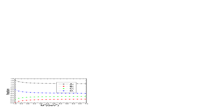
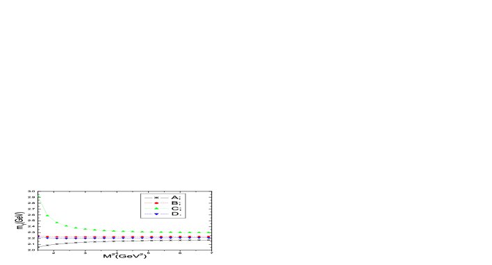
From Figs.1-2, we can see that the main contribution comes from the perturbative term, the hadronic spectral density above and below the threshold can be successfully approximated by the perturbative term. If we take typical values for the parameters $\sqrt{s_{0}}=2.4GeV$ and $M^{2}=4.0GeV^{2}$, the contributions from continuum states are dominating,

$\displaystyle\frac{\int_{0}^{s_{0}}dtt^{4}e^{-t/M^{2}}}{\int_{0}^{\infty}dtt^{4}e^{-t/M^{2}}}<2\%\,.$ (15)

It is not an indication that non-existence of the tetraquark states due to lack experimental information about physics above the threshold $s_{0}$. One may refuse the value extracted from continuum dominating QCD sum rules as quantitatively reliable if one insists on that contribution from the pole term should be larger than (or about) $50\%$ in conventional QCD sum rules.

In this article, we cannot find the conventional Borel window (or the Borel window is too small to make robust prediction) and threshold parameter for the sum rule in Eq.(11); and release standard criterion and prefer more phenomenological analysis. We choose the suitable values for the Borel parameter $M$, on the one hand, the minimal values $M_{min}$ are large enough to warrant the convergence of operator product expansion, for $M_{min}>\sqrt{3}GeV$, the dominating contribution comes from the perturbative term in Eq.(11), larger than $90\%$; on the other hand, the maximal values $M_{max}$ are small enough to suppress the contributions from the high resonance (or excited) states and continuum states, we choose naive analysis $e^{-s_{0}/(M_{max})^{2}}\leq e^{-1}$.

Refer to caption
Figure 1: Fractions of different terms with Borel parameter $M^{2}$ in the right hand side of Eq.(11). $A$, $B$, $C$ and $D$ stand for the contributions from the terms proportional to $t^{4}$, ⟨s¯​s⟩delimited-βŸ¨βŸ©Β―π‘ π‘ \langle\bar{s}s\rangle, ⟨s¯​sβŸ©β€‹βŸ¨s¯​gs​σ​G​s⟩delimited-βŸ¨βŸ©Β―π‘ π‘ delimited-βŸ¨βŸ©Β―π‘ subscriptπ‘”π‘ πœŽπΊπ‘ \langle\bar{s}s\rangle\langle\bar{s}g_{s}\sigma Gs\rangle and ⟨s¯​s⟩2superscriptdelimited-βŸ¨βŸ©Β―π‘ π‘ 2\langle\bar{s}s\rangle^{2}, respectively. The contributions from the terms of minor importance (less than $10\%$) are not shown explicitly. The input parameters are taken as $\sqrt{s_{0}}=2.4GeV$, and central values of the vacuum condensates.
Refer to caption
Figure 2: Mass from different terms with Borel parameter $M^{2}$ in Eq.(13), $A$, $B$, $C$ and $D$ from the terms proportional to $t^{4}$, t4+⟨s¯​s⟩superscript𝑑4delimited-βŸ¨βŸ©Β―π‘ π‘ t^{4}+\langle\bar{s}s\rangle, t4+⟨s¯​s⟩+⟨s¯​sβŸ©β€‹βŸ¨s¯​gs​σ​G​s⟩superscript𝑑4delimited-βŸ¨βŸ©Β―π‘ π‘ delimited-βŸ¨βŸ©Β―π‘ π‘ delimited-βŸ¨βŸ©Β―π‘ subscriptπ‘”π‘ πœŽπΊπ‘ t^{4}+\langle\bar{s}s\rangle+\langle\bar{s}s\rangle\langle\bar{s}g_{s}\sigma Gs\rangle and t4+⟨s¯​s⟩+⟨s¯​sβŸ©β€‹βŸ¨s¯​gs​σ​G​s⟩+⟨s¯​s⟩2superscript𝑑4delimited-βŸ¨βŸ©Β―π‘ π‘ delimited-βŸ¨βŸ©Β―π‘ π‘ delimited-βŸ¨βŸ©Β―π‘ subscriptπ‘”π‘ πœŽπΊπ‘ superscriptdelimited-βŸ¨βŸ©Β―π‘ π‘ 2t^{4}+\langle\bar{s}s\rangle+\langle\bar{s}s\rangle\langle\bar{s}g_{s}\sigma Gs\rangle+\langle\bar{s}s\rangle^{2}, respectively. The contributions from the terms of minor importance are not shown explicitly. The input parameters are taken as $\sqrt{s_{0}}=2.4GeV$, and central values of the vacuum condensates.

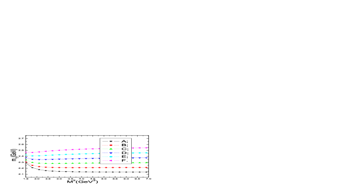
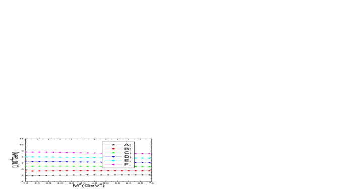
In Figs.3-4, we plot the values of the mass $m_{Y}$ and decay constant $f_{Y}$ with variation of the threshold parameter $s_{0}$. From those figures, we can see that the values increase steadily with increase of $s_{0}$, the QCD sum rules cannot indicate existence of the tetraquark state $Y(2175)$ strictly, we should adopt more phenomenological analysis.

The vector current $J^{c}_{\mu}=\bar{c}\gamma_{\mu}c$ can interpolate the vector mesons $J/\psi(1S)$, $\psi(2S)$, $\psi(3770)$, $\psi(4040)$, $\psi(4160)$ and $\psi(4415)$, the correlation function Πμ​νcsubscriptsuperscriptΞ π‘πœ‡πœˆ\Pi^{c}_{\mu\nu},

Πμ​νc=iβ€‹βˆ«d4​x​ei​pβ‹…xβ€‹βŸ¨0|T​{JΞΌc​(x)​JΞ½c​(0)}|0⟩,subscriptsuperscriptΞ π‘πœ‡πœˆπ‘–superscript𝑑4π‘₯superscript𝑒⋅𝑖𝑝π‘₯quantum-operator-product0𝑇subscriptsuperscriptπ½π‘πœ‡π‘₯subscriptsuperscriptπ½π‘πœˆ00\displaystyle\Pi^{c}_{\mu\nu}=i\int d^{4}xe^{ip\cdot x}\langle 0|T\left\{J^{c}_{\mu}(x)J^{c}_{\nu}(0)\right\}|0\rangle\,, (16)

can be saturated by $J/\psi(1S)$, $\psi(2S)$, $\psi(3770)$, $\psi(4040)$, $\psi(4160)$, $\psi(4415)$ and continuum states at the phenomenological side [18]. The masses and widths of those vector mesons are well known, one can consult PDG for details [19]. If experimental data about the higher resonances $Y_{1}$, $Y_{2}$, $\cdots$ are available (suppose there are some), we can make analogous analysis as in the vector hidden charm channels to avoid difficulty in choosing the Borel parameter $M^{2}$ and threshold parameter $s_{0}$.

However, present experimental knowledge about the phenomenological hadronic spectral densities of the multiquark states is rather vague, even existence of the multiquark states is not confirmed with confidence, and no knowledge about either there are high resonances or not. Criterion in Eq.(14) cannot lead to reasonable Borel parameter $M$ and threshold parameter $s_{0}$ for the multiquark states, we can either reject the QCD sum rules for the multiquark states or release the condition, we are optimistical participators333We take the point of view that although the standard criterion of the QCD sum rules cannot be satisfied for the multiquark states, experimental data about the high resonances is of great importance; we should analyze the ground state and high resonances together and come out the difficulty. .

In this article, we approximate the spectral density with the contribution from the single-pole term, the threshold parameter $s_{0}$ is taken slightly above the ground state mass ( $\sqrt{s_{0}}>m_{Y}+\frac{\Gamma_{Y}}{2}$) to subtract the contributions from the high resonances and continuum states. We take $\sqrt{s_{0}}=(2.3-2.5)GeV>2.2GeV$, it is reasonable for Breit-Wigner mass $m_{Y}=2.175\pm 0.010\pm 0.015GeV$ and width $\Gamma_{Y}=58\pm 16\pm 20MeV$. The Borel parameter $M$ can be chosen to be $M^{2}=(3.0-7.0)GeV^{2}$, in this region, the values of the mass and decay constant are rather stable with respect to variation of the Borel parameter, which are shown in Fig.3 and Fig.4 respectively.

Refer to caption
Figure 3: $m_{Y}$ with the central values of the vacuum condensates. $A$, $B$, $C$, $D$, $E$ and $F$ stand for $\sqrt{s_{0}}=$ $2.3GeV$, $2.4GeV$, $2.5GeV$, $2.6GeV$, $2.7GeV$ and $2.8GeV$ respectively.
Refer to caption
Figure 4: $f_{Y}$ with the central values of the vacuum condensates. $A$, $B$, $C$, $D$, $E$ and $F$ stand for $\sqrt{s_{0}}=$ $2.3GeV$, $2.4GeV$, $2.5GeV$, $2.6GeV$, $2.7GeV$ and $2.8GeV$ respectively.

Finally, we obtain the values of the mass and decay constant of $Y(2175)$,

$\displaystyle m_{Y}$ $\displaystyle=$ $\displaystyle(2.21\pm 0.09)GeV\,,$
$\displaystyle f_{Y}$ $\displaystyle=$ $\displaystyle(5.78\pm 0.89)10^{-4}GeV\,.$ (17)

The main uncertainty comes from the threshold parameter $s_{0}$, uncertainties of the vacuum condensates and mssubscriptπ‘šπ‘ m_{s} can only lead to minor uncertainty.

If we take smaller values for the Borel parameter $M^{2}$ and larger values for the threshold parameter $s_{0}$, for example, $M^{2}=(1.5-3.0)GeV^{2}$ and $\sqrt{s_{0}}=(2.3-2.9)GeV$, the contribution from the pole term (or ground state) can be greatly enhanced, which is shown in table.1. From the table, we can see that if we take $M^{2}=(1.5-2.0)GeV^{2}$ and $\sqrt{s_{0}}=(2.6-2.8)GeV$ , the contribution from the pole term (or ground state) is about $(25-60)\%$, the phenomenological spectral density can be roughly approximated by the ”single-pole $+$ continuum states” model 444 The Borel window is rather small, that may impair the predicative ability. . Taking into account all the uncertainties, we obtain the values of the mass and decay constant from Eqs.(11-13)

$\displaystyle m_{Y}$ $\displaystyle=$ $\displaystyle(2.46\pm 0.16)GeV\,,$
$\displaystyle f_{Y}$ $\displaystyle=$ $\displaystyle(8.06\pm 0.87)10^{-4}GeV\,.$ (18)
$M^{2}(GeV^{2})$ $\mbox{Pole}(\%)$ $\sqrt{s_{0}}(GeV)$ $m_{Y}(GeV)$
$1.5-2.0$ $13-28$ $2.3$ $1.98-2.02$
$1.5-2.0$ $16-34$ $2.4$ $2.05-2.09$
$1.5-2.0$ $21-40$ $2.5$ $2.12-2.17$
$1.5-2.0$ $25-47$ 2.6 $2.18-2.24$
$1.5-2.0$ $30-53$ $2.7$ $2.25-2.32$
$1.5-2.0$ $36-60$ $2.8$ $2.30-2.39$
$1.5-2.0$ $41-66$ $2.9$ $2.36-2.45$
$2.5-3.0$ $8-14$ $2.6$ $2.28-2.30$
$2.5-3.0$ $10-17$ $2.7$ $2.35-2.38$
$2.5-3.0$ $12-21$ $2.8$ $2.43-2.46$
$2.5-3.0$ $15-25$ $2.9$ $2.50-2.53$
Table 1: The relation among the Borel parameter, pole term (or ground state) contribution, threshold parameter and mass with the spectral density approximated by the perturbative term.

4 Conclusion

In this article, we take the point of view that $Y(2175)$ be a tetraquark state which consists of color octet constituents, and calculate its mass and decay constant within the framework of the QCD sum rules approach. We release standard criterion in the QCD sum rules approach and take more phenomenological analysis, the value of the mass of $Y(2175)$ is consistent with experimental data; there may be some tetraquark components in the state $Y(2175)$. On the other hand, if we retain standard criterion and take a rather small Borel window, larger mass than the experimental data can be obtained, the current $J_{\mu}(x)$ can interpolate a tetraquark state with larger mass, or $Y(2175)$ has some components with larger mass. More experimental data are needed to select the ideal sum rule for the tetraquark states. We can take color octet operators as basic constituents in constructing the tetraquark currents, because the perturbative term may have dominant contribution, in other words, the tetraquark states may consist of color octet constituents rather than diquark pairs.

Acknowledgments

This work is supported by National Natural Science Foundation, Grant Number 10405009, and Key Program Foundation of NCEPU.

References

  • [1] B. Aubert, et al, Phys. Rev. D74 (2006) 091103.
  • [2] M. A. Shifman, A. I. Vainshtein and V. I. Zakharov, Nucl. Phys. B147 (1979) 385, 448; L. J. Reinders, H. Rubinstein and S. Yazaki, Phys. Rept. 127 (1985) 1.
  • [3] S. Narison, QCD Spectral Sum Rules, World Scientific Lecture Notes in Physics 26 (1989) 1.
  • [4] P. Colangelo and A. Khodjamirian, hep-ph/0010175.
  • [5] L. Maiani, F. Piccinini, A. D. Polosa, V. Riquer, Phys. Rev. D72 (2005) 031502; Phys. Rev. D71 (2005) 014028; Phys. Rev. Lett. 93 (2004) 212002.
  • [6] F. E. Close and N. A. Tornqvist, J. Phys. G28 (2002) R249; and references therein.
  • [7] R. L. Jaffe, Phys. Rept. 409 (2005) 1; C. Amsler and N. A. Tornqvist, Phys. Rept. 389 (2004) 61; and references therein.
  • [8] T. V. Brito, F. S. Navarra, M. Nielsen, M. E. Bracco, Phys. Lett. B608 (2005) 69; H. J. Lee, N. I. Kochelev, Phys. Lett. B642 (2006) 358; H. X. Chen, A. Hosaka, S. L. Zhu, Phys. Rev. D74 (2006) 054001.
  • [9] Z. G. Wang, W. M. Yang and S. L. Wan, J. Phys. G31 (2005) 971; Z. G. Wang and W. M. Yang, Eur. Phys. J. C42 (2005) 89.
  • [10] R. D. Matheus, S. Narison, M. Nielsen, J. M. Richard, Phys. Rev. D75 (2007) 014005; M. E. Bracco, A. Lozea, R. D. Matheus, F. S. Navarra and M. Nielsen, Phys. Lett. B624 (2005) 217; H. Kim and Y. Oh, Phys. Rev. D72 (2005) 074012; F. S. Navarra, M. Nielsen , Phys. Lett. B639 (2006) 272.
  • [11] Z. G. Wang, S. L. Wan, Nucl. Phys. A778 (2006) 22; Z. G. Wang, S. L. Wan, J. Phys. G34 (2007) 505; Z. G. Wang, S. L. Wan, Chin. Phys. Lett. 23 (2006) 3208.
  • [12] J. I. Latorre and P. Pascual, J. Phys. G11 (1985) L231; S. Narison, Phys. Lett. B175 (1986) 88.
  • [13] N. Kodama, M. Oka and T. Hatsuda, Nucl. Phys. A580 (1994) 445.
  • [14] R. D. Matheus and S. Narison, hep-ph/0412063; W. Wei, P. Z. Huang, H. X. Chen, S. L. Zhu, JHEP 0507 (2005) 015; Z. G. Wang, S. L. Wan and W. M. Yang, Eur. Phys. J. C45 (2006) 201.
  • [15] B. L. Ioffe, K. N. Zyablyuk, Nucl. Phys. A687 (2001) 437; B. V. Geshkenbein, B. L. Ioffe, K. N. Zyablyuk, Phys. Rev. D64 (2001) 093009; K. Zyablyuk, JHEP 0301 (2003) 081.
  • [16] B. L. Ioffe, Prog. Part. Nucl. Phys. 56 (2006) 232; and references therein.
  • [17] M. Davier, A. Hocker, Z. Zhang, Rev. Mod. Phys. 78 (2006) 1043; and references therein.
  • [18] B. L. Ioffe, K. N. Zyablyuk, Eur. Phys. J. C27 (2003) 229; M. Eidemuller, M. Jamin, Phys. Lett. B498 (2001) 203.
  • [19] W. M. Yao, et al, J. Phys. G33 (2006) 1.