The Charm Quark Contribution to the Proton Structure Function

Abstract

The charm quark structure function $F^{c}_{2}$ and the longitudinal structure function $F_{l}^{p}$ are directly sensitive to the gluon content of proton and therefore are crucial in understanding of proton structure function, in particular at low momentum transfer $Q^{2}$ and low Bjorken x. In the framework of perturbative QCD the charm structure function is calculated in the leading order (LO) and the proton structure function is investigated in the next leading order (NLO) at small x region. The valence quark distribution is obtained from the relativistic quark-exchange model. The calculated $F_{2}^{c}(x,Q^{2})$, $F_{2}^{p}(x,Q^{2})$ and $F_{L}^{p}(x,Q^{2})$, are compared with the present available experimental data.

I Valence Quark Distribution

In the evaluation of valence quark distribution, we assumed that the nucleon is composed of three valence-quarks in the following way ref1 :

$$|{\alpha}{\rangle}={\cal N}^{{\alpha}^{\dagger}}|0{\rangle}={1\over\sqrt{3!}}{\cal N}^{\alpha}_{{\mu}_{1}{\mu}_{2}{\mu}_{3}}q^{\dagger}_{{\mu}_{1}}q^{\dagger}_{{\mu}_{2}}q^{\dagger}_{{\mu}_{3}}|0{\rangle},$$ (1)

where $\alpha$ designate the nucleon states ${\{\vec{P}},M_{S},M_{T}\}$ and ${\mu}$ stand for the quark states ${\{\vec{k}},m_{s},m_{t},c\}$. With the convention that there is a summation on the repeated indices as well as integration over $\vec{k}$. $q^{\dagger}$ $({\cal N}^{{\alpha}^{\dagger}})$ are the creation operators for quarks (nucleons) and ${\cal N}^{\alpha}_{{\mu}_{1}{\mu}_{2}{\mu}_{3}}$ are the totally antisymmetric nucleon wave functions, i.e.

$${\cal N}^{\alpha}_{{\mu}_{1}{\mu}_{2}{\mu}_{3}}=D(\mu_{1},\mu_{2},\mu_{3};\alpha_{i})\times{\delta({\vec{k}_{1}}+{\vec{k}_{2}}+{\vec{k}_{3}}-{\vec{P}}})$$

$$\times{\phi({\vec{k}_{1}},{\vec{k}_{2}},{\vec{k}_{3}},{\vec{P}})}.$$ (2)

The $D(\mu_{1},\mu_{2},\mu_{3};\alpha_{i})$ depend on the Clebsch-Gordon coefficients $C^{{j_{1}}{j_{2}}{j}}_{{m_{1}}{m_{2}}{m}}$ and the color factor $\epsilon_{{c_{1}}{c_{2}}{c_{3}}}$,

$$D(\mu_{1},\mu_{2},\mu_{3};\alpha_{i})={1\over\sqrt{3!}}\epsilon_{c_{1}c_{2}c_{3}}{1\over\sqrt{2}}\sum_{s,t=0,1}C^{{1\over 2}s{1\over 2}}_{m_{s_{\sigma}}m_{s}M_{S_{\alpha_{i}}}}C^{{1\over 2}{1\over 2}s}_{m_{s_{\mu}}m_{s_{\nu}}m_{s}}C^{{1\over 2}t{1\over 2}}_{m_{t_{\sigma}}m_{t}M_{T_{\alpha_{i}}}}C^{{1\over 2}{1\over 2}t}_{m_{t_{\mu}}m_{t_{\nu}}m_{t}}$$ (3)

The ${\phi({\vec{k}_{1}},{\vec{k}_{2}},{\vec{k}_{3}},{\vec{P}})}$ are the nucleon wave functions in terms of quarks and we write it in a Gaussian form (b $\simeq$ nucleon radius) :

$$\phi({\vec{k}_{1}},{\vec{k}_{2}},{\vec{k}_{3}},{\vec{P}})={\left(\frac{3b^{4}}{{\pi}^{2}}\right)^{3\over 4}}\times~{}~{}~{}~{}~{}~{}~{}~{}~{}~{}~{}~{}~{}~{}~{}~{}~{}~{}~{}~{}~{}~{}~{}~{}$$

$$\exp[-b^{2}(\frac{(k_{1}^{2}+k_{2}^{2}+k_{3}^{2})}{2}+\frac{{b^{2}}{P^{2}}}{6}].$$ (4)

We can define the nucleus state based on nucleon creation operators, i.e.

$$|{\cal A}_{i}=3{\rangle}={(3!)^{-{1\over 2}}}{\chi}^{{\alpha}_{1}{\alpha}_{2}{\alpha}_{3}}{\cal N}^{{{\alpha}_{1}}^{\dagger}}{\cal N}^{{{\alpha}_{2}}^{\dagger}}{\cal N}^{{{\alpha}_{3}}^{\dagger}}|0{\rangle},$$ (5)

where ${\chi}^{{\alpha}_{1}{\alpha}_{2}{\alpha}_{3}}$ are the complete antisymmetric nuclear wave functions (they are taken from Faddeev calculations with Reid soft core potential.

The quark momentum distributions with fixed flavour in a three nucleon system are defined as,

$${\rho}_{\bar{\mu}}(\vec{k};{\cal A}_{i})={{\langle}{\cal A}_{i}=3|q^{\dagger}_{\bar{\mu}}q_{\bar{\mu}}|{\cal A}_{i}=3{\rangle}\over{\langle}{\cal A}_{i}=3|{\cal A}_{i}=3{\rangle}}~{}~{}~{}~{}~{},$$ (6)

where the sign bar means no summation on $m_{t}$ and integration over $\vec{k}$ in the $\mu$ indices. By using the above definition, we can calculate the quark momentum distribution for each flavour. In the above equation we use, $\chi(x,y,cos\theta)$, the Fourier transform of the nucleus wave function.

By considering the relativistic correction, the valence parton distribution at each $Q^{2}$ can be related to momentum distribution for each flavour according to the following equation,

$$q^{v}(x,Q^{2};{\cal A}_{i})={1\over(1-x)^{2}}\int\rho_{q}({\vec{k}};{\cal A}_{i})\times~{}~{}~{}~{}~{}~{}~{}~{}~{}~{}~{}~{}~{}~{}~{}$$

$$\delta({x\over(1-x)}-{k_{+}\over M})\ d{\vec{k}}.$$ (7)

Evaluating the angular integration, we find that,

$$q^{v}(x,Q^{2};{\cal A}_{i})={{2\pi M}\over{(1-x)^{2}}}{\int_{k_{min}}^{\infty}}\rho_{q}({\vec{k}};{\cal A}_{i})k\ dk$$ (8)

with

$$k_{min}(x)={{({{xM}\over{1-x}}+\epsilon_{0})^{2}-m^{2}}\over{2({{xM}\over{1-x}}+\epsilon_{0})}},$$ (9)

where m (M) is the quark (nucleon) mass , $k_{+}$ is the light-cone momentum of initial quark and $\epsilon_{0}$ is the quark binding energy. The valence quark distribution of a bound nucleon can be derived from the free nucleon valence quark distribution function by using the convolution approximation,

$$q^{v}(x,Q^{2};{\cal A}_{i})=\sum_{N}\int q^{v}({x\over y_{{\cal A}_{i}}},Q^{2};N)f_{N/{\cal A}_{i}}(y_{{\cal A}_{i}})\ d{y_{{\cal A}_{i}}},$$ (10)

where $f_{N/{\cal A}_{i}}(y_{{\cal A}_{i}})$ are the nucleon momentum distributions in the nucleus. By taking into account the fact that $f_{N/{\cal A}_{i}}(y_{{\cal A}_{i}})$ are large only around $x\over{\langle y_{{\cal A}_{i}}\rangle}$ we can write [23]

$$\Delta q^{v}({x\over{\langle y_{{\cal A}_{i}}\rangle}},Q^{2};N)=\Delta q^{v}(x,Q^{2};{\cal A}_{i})$$ (11)

with ${\langle y_{{\cal A}_{i}}\rangle}=1+{{\bar{\epsilon}}\over M}$ and $\bar{\epsilon}$ being the average removal energy of the nucleon. A typical ansatz for the parton distribution is usually parameterized as,

$$x~{}{\cal P}(x,Q^{2})=A_{\cal P}{\eta_{\cal P}}x^{a_{\cal P}}(1-x)^{b_{\cal P}}(1+\gamma_{\cal P}x+\varrho_{\cal P}x^{1\over 2})$$ (12)

where $A_{\cal P}$ is the normalization factor.

II NLO Evolution Procedure

It is appropriate to use the Mellin and inverse Mellin transformation to calculate the NLO parton distributions in the $(x,Q^{2})$-plane ref1 .

In the NLO, $F^{p}_{2}(x,Q^{2})$ is related to the quark, antiquark and gluon distributions, as follows:

$$F^{p}_{2}(x;Q^{2})=x\sum_{q=u,d,s}{e_{q}^{2}}\{q(x,Q^{2})+{\bar{q}}(x,Q^{2})\}+{\alpha_{s}(Q^{2})\over 2\pi}[C_{q}\otimes({q(x,Q^{2})+{\bar{q}}^{N}(x,Q^{2}})+{2}C_{g}\otimes G(x,Q^{2})]+F_{2}^{c}(x,Q^{2},m_{c}^{2}),$$ (13)

where $\otimes$ means the convolution and it is defined as,

$$C_{\cal P}\otimes{\cal P}=\int_{x}^{1}{\ dy\over y}C_{\cal P}({x\over y}){\cal P}(y,Q^{2}).$$ (14)

The charm quark contribution to the proton structure function $F_{2}^{c}(x,Q^{2},m_{c}^{2})$ has the following form in the LO limit, if ${1\over x}\geq 1+({2m_{c}\over Q})^{2}$, (note that for small x, with this condition $Q^{2}$ can become less than $m^{2}_{c}$,

$$F_{2}^{c}(x,Q^{2},m_{c}^{2})=2xe^{2}_{c}{\alpha_{s}({\mu^{\prime}}^{2})\over 2\pi}\int_{ax}^{1}{dy\over y}C^{c}_{g}({x\over y},({m_{c}\over Q})^{2})$$

$$\times g(y,{\mu^{\prime}}^{2})~{}~{}~{}~{}~{}~{}~{}$$ (15)

where $a=1+4{m_{c}^{2}\over Q^{2}}$ and ($n_{f}$ is the number of active flavours)

$$\alpha_{s}(Q^{2})={4\pi\over\beta_{0}\ln(Q^{2}/\Lambda^{2})}-{4\pi\beta_{1}\over\beta_{0}^{3}}{\ln\ln(Q^{2}/\Lambda^{2})\over\ln(Q^{2}/\Lambda^{2})}$$ (16)

with ($\Lambda_{\overline{MS}}=200MeV$)

$$\beta_{0}=11-{2\over 3}n_{f},\ \ \ \beta_{1}=102-{38\over 3}n_{f}.$$ (17)

The longitudinal SF,$F^{p}_{L}(x;Q^{2})$ is obtained as:

$$F^{p}_{L}(x;Q^{2})=x{\alpha_{s}(Q^{2})\over 2\pi}\sum_{q=u,d,s}[C_{q,L}\otimes({q(x,Q^{2})+{\bar{q}}^{N}(x,Q^{2}})+{2}C_{g,L}\otimes G(x,Q^{2})]+F_{L}^{c}(x,Q^{2},m_{c}^{2})$$ (18)

with

$$C_{q,L}={8\over 3}z,\ \ C_{g,L}=2z(z-1).$$ (19)

We use the LO expression for $F_{L}^{c}(x,Q^{2},m_{c}^{2})$, which is the same as equation (3) i.e.

$$F_{L}^{c}(x,Q^{2},m_{c}^{2})=2xe^{2}_{c}{\alpha_{s}({\mu^{\prime}}^{2})\over 2\pi}\int_{ax}^{1}{dy\over y}C^{c}_{g,L}({x\over y},({m_{c}\over Q})^{2})$$

$$\times g(y,{\mu^{\prime}}^{2})~{}~{}~{}~{}~{}~{}~{}$$ (20)

Here we assume the SU(3) flavour-symmetric sea quark distributions ${\bar{q}}={\bar{u}}={\bar{d}}={\bar{s}}={s}$. In addition we consider the sea quark and gluon contributions to vanish in the static point $\mu_{0}^{2}\ll Q^{2}$, ( we set $\mu_{0}^{2}=0.32GeV^{2}$),i.e,

$$G(x,\mu_{0}^{2})=0~{}~{}~{}~{}~{}~{}~{}~{}~{}~{}~{}~{}~{}~{}~{}\bar{q}(x,\mu_{0}^{2})=0.$$ (21)

Note that, this is the scale where the above initial condition is approximately satisfied i.e. the $\mu_{0}^{2}$ scale is determined from the intermediate $Q^{2}_{0}$ scale by evolving downward the second moment of the valence quark distributions such that the gluon and sea quark distributions are approximately zero at the $\mu_{0}^{2}$ scale.

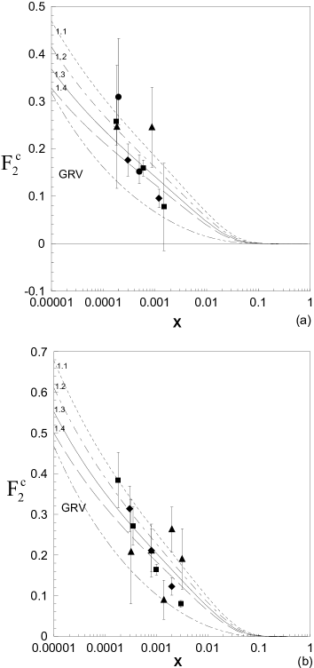
Figure 1: The charm contribution to the proton structure function at (a) $Q^{2}=6GeV^{2}$ and (b) $Q^{2}=10GeV^{2}$ for various charm mass. The data are from various ZEUS and H1 collaborations experiments.

III Results and discussions

In figure 1, we present the charm quark contribution to the Structure function of proton at ( $Q^{2}=6GeV^{2}$) with different charm mass values i.e. $m_{c}=1.1GeV$ (small-dash curve), $m_{c}=1.2GeV$ (dash-small-dash curve), $m_{c}=1.3GeV$( full curve) and $m_{c}=1.4GeV$ (dash curve). The data are those of H1 ref2 and ZEUS collaborations ref3 , i.e. the squares (ZEUS,1997), circles (H1,2000), diamonds (ZEUS,2000) and triangles (ZEUS,2004). Our results are in very good agreement with the present available data. By reducing the charm mass, the charm structure function of proton increases but it still passes though the data. It also becomes zero for $x>0.1$. Obviously the structure function becomes larger as we increase $Q^{2}$. The calculated $F_{2}^{c}(x,Q^{2})$ by using the gluon distribution of GRV (heavy-full curves) with $m_{c}=1.3$ shows less charm quark contribution to the structure function of proton.

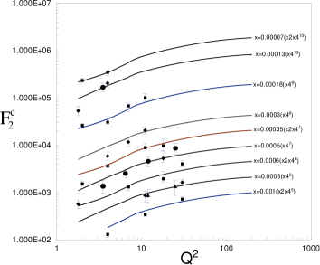
Figure 2: The $Q^{2}(GeV^{2})$ dependence of charm contribution to SF of proton for the various x values. The data are from ZEUS [2] and H1 [3] collaboration experiments.

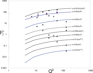
Figure 3: As figure. 2.

Figures 2 and 3 show the comparison of $Q^{2}$ dependence of charm contribution to the structure function of proton for various x values with the available ZEUS data (the triangles (1997), circles (2000) and squares (2004)). We get a reasonable result with respect to the data [2].

The $Q^{2}$ dependence of longitudinal structure function of proton are given in figure 4. The data are from H1 collaboration experiments: the circles (H1,2001) and triangles (H1,1996). Again there are a good agreement between our calculated results and the experimental predictions data. These show that our gluon distribution can reasonably well treat the PGF process.

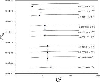
Figure 4: The $Q^{2}(GeV^{2})$ dependence of longitudinal SF of Proton. The data are from H1 collaboration experiments.

We have observed a linear $Q^{2}$-dependence in the unpolarized structure function which is in a very good agreement with the available data. A smooth behavior was found for the sea-quark and gluon distribution functions. The agreement between our uniquely gluon and sea quarks distributions and the available data are encouraging. In particular we fully reproduced the gluon distribution. We note that the above assumption where the gluon and the sea-quark distributions can be generated entirely radiatively from valence quark may not be valid, especially at small x.

In summary, by using our recent complete NLO calculation in the conventional $\overline{MS}$ factorization scheme, we have updated our previous NLO results by including the charm contribution to the SF of proton. We have found that the proton structure function has approximately the same $Q^{2}$-dependence as the data and the whole results are consistent with the available experiments. Our calculation shows a similar scaling violation as the one observed in the experiment for the small x. The idea that at low x the scaling violation of $F^{N}_{2}(x,Q^{2})$ comes from the gluon density alone and does not depend on the quark density which was tested in our previous work, is still valid with a good accuracy. So, as before, we may conclude that the gluon is the dominant source of the parton in the small x region. However, it is well known that the theoretical interpretation of SF is complicated at low $Q^{2}$. Since, in this region the higher twist contributions which are proportional to $Q^{-2}$ and $Q^{-4}$ are not included in the DGLAP equations.

References

(1)M. M. Yazdanpanah and M. Modarres, Eur.Phys.J.A, 7
(2000) 573.
M. M. Yazdanpanah and. M. Modarres, Eur.Phys.J.A, 6 (1999) 91.
(2)H1 collaboration, T. Ahmed et al, Nucl.Phys.B, 439 (1995)
471; S. Aid et al, Nucl.Phys.B, 445 (1996) 3; I. Abt et al.,
Nucl.Phys., B407 (1993) 515; C. Adloff et al , Eur.Phys.J.C, 19
(2001) 269; Eur. Phys. J. C21 (2001) 33; Eur. Phys.J.C, 13 (2000)
609; A. Aktas et al., Phys.Lett.B, 598 (2004) 159 and Phys.Lett.
B407 (2002) 402.
(3)ZEUS collaboration, M. Derrick et al., Z.Phys.C, 72 (1996) 399;
M. Derrick et al., Phys.Lett.B, 316 (1993) 412 and Phys.Lett.B,
407 (1997) 402; J. Breitwag et al., Euro.Phys.J.C 12 (2000) 35 and
Eur.Phys.J.C, 7 (1999) 609; S. Chekanov et al., Phys.Rev.D, 69
(2004) 012004; S.Chekanov et al, Eur.Phys.J.C, 21 (2001) 443.