NUMERICALLY STABLE CALCULATIONS OF RADIATIVE CORRECTIONS TO BREMSSTRAHLUNG IN $e^{+}e^{-}$ ANNIHILATION

Abstract

We discuss techniques for obtaining a numerically stable evaluation of the fully differential cross section for the virtual photon correction to single hard photon bremsstrahlung in two different computational schemes. We also compare the role of finite mass corrections in these schemes.

BU-HEPP-06/09

1 Introduction

Electron-positron annihilation to fermions, $e^{+}e^{-}\rightarrow f{\overline{f}}$, plays a critical role in extracting precision electroweak physics from $e^{+}e^{-}$ colliders. Precise calculations are needed for the final data analysis of LEP and the anticipated ILC. Thus, the basic process must be augmented by radiative effects, in particular bremsstrahlung from a fermion line, $e^{+}e^{-}\rightarrow f{\overline{f}}\gamma$. More photons may be added as needed, including virtual photons exchanged in internal lines to the desired order. Single hard bremstrahlung is also of importance in “radiative return” experiments, where the radiated photon is used to reduce the effective energy of the collision, permitting a range of energies to be studied at a fixed-energy accelerator. This technique is useful at B factories and high-energy colliders.

In this note, we will be concerned with the accurate calculation of one-loop corrections to single real photon emissions, where there is one extra virtual photon in the process.[1] We will discuss some aspects of calculating these corrections in a manner stable enough to permit high-precision Monte Carlo comparisons to related results.[2, 3] We will also discuss the role of finite-mass corrections, and compare our approach to that of Ref. [3], examining the role of mass corrections in the level of agreement found for these results.

2 Virtual Corrections to Bremsstrahlung

The one-loop virtual correction to initial or final-state bremsstrahlung was calculated in Ref. [1] using helicity spinor methods, which provide an efficient representation of massless fermion scattering, including a “magic” choice for the photon polarization vectors which eliminates many terms from the calculation.[4, 5, 6] The amplitudes were simplified using the symbolic manipulation FORM,[7] and the scalar one-loop Feynman integrals were evaluated using the FF package.[8] Eventually, these integrals were replaced by the analytic expressions in Ref. [1] as shown in the appendix of that paper. The amplitudes are then evaluated by the ${\cal KK}$ Monte Carlo program,[9] which squares and sums them numerically when creating events to obtain the scattering cross section.

The initial state virtual photon contribution to the cross-section may be expressed as

$$\frac{{d\sigma}^{(1)}_{1}}{d\Omega dr_{1}dr_{2}}=\frac{1}{(8\pi)^{4}}\sum_{\lambda_{i},\sigma}2\,{\rm Re}\left[({\cal M}^{(0)}_{1})^{*}{\cal M}^{(1)}_{1}\right]$$ (1)

where the tree-level result is

$$\frac{{d\sigma}^{(0)}_{1}}{d\Omega dr_{1}dr_{2}}=\frac{1}{(8\pi)^{4}}\sum_{\lambda_{i},\sigma}\left|{\cal M}^{(0)}_{1}\right|^{2}$$ (2)

with summed-squared matrix element

$$\sum_{\lambda_{i},\sigma}\left|{\cal M}^{(0)}_{1}\right|^{2}=\frac{16e^{6}}{s^{2}s^{\prime}r_{1}r_{2}}\left\{\left(t_{1}^{2}+u_{1}^{2}\right)\left(1-\frac{2m_{e}^{2}r_{1}}{s^{\prime}r_{2}}\right)+\left(t_{2}^{2}+u_{2}^{2}\right)\left(1-\frac{2m_{e}^{2}r_{2}}{s^{\prime}r_{1}}\right)\right\},$$ (3)

with $s=(p_{1}+p_{2})^{2}$, $s^{\prime}=(p_{3}+p_{4})^{2}$, $t_{1}=(p_{1}-p_{3})^{2}$, $t_{2}=(p_{2}-p_{4})^{2}$, $u_{1}=(p_{1}-p_{4})^{2}$, $u_{2}=(p_{2}-p_{3})^{2}$, $r_{i}=2p_{i}\cdot k/s$, where $p_{1},p_{2},p_{3},p_{4},k$ are the momenta of the $e^{-},e^{+},f,{\overline{f}},$ and $\gamma$. The explicit mass corrections in Eq. 3 are obtained using the method of Ref. [12], as discussed in Sec. 3. The matrix element for hard photon initial-state emission with one virtual photon may be expressed as

$${\cal M}^{(1)}_{1}=\frac{\alpha}{4\pi}{\cal M}^{(0)}_{1}(f_{0}+f_{1}I_{1}+f_{2}I_{2}),$$ (4)

where $f_{i}$ are scalar form factors and $I_{i}$ are spinor factors defined in Ref. [1].

The expressions for the $f_{i}$ include differences between logarithms and dilogarithms with arguments which are very similar in collinear limits, and these differences are frequently divided by the collinear factors $r_{i}$, so that the result is finite in the collinear limits. Evaluating such expressions in a numerically stable manner requires expansions where appropriate. A set of functions useful for this purpose are the logarithmic and dilogarithmic difference functions ${\rm Lf}_{n}(x)$ and ${\rm Sf}_{n}(x,y)$ introduced in Refs. [10, 11] and defined recursively via

$${\rm Lf}_{0}(x) = \ln(1+x),$$

$${\rm Lf}_{n+1}(x) = \frac{1}{x}\left({\rm Lf}_{n}(x)-{\rm Lf}_{n}(0)\right),$$

$${\rm Sf}_{0}(x,y) = {\rm Sp}\;(x+y),$$ (5)

$${\rm Sf}_{n+1}(x,y) = \frac{1}{y}\left({\rm Sf}_{n}(x,y)-{\rm Sf}_{n}(x,0)\right),$$

with ${\rm Sp}\;(x)$ the dilogarithm (Spence function). A set of identities and expansions for these functions may be found in the appendix of Ref. [11]. Thus, for example, the form factor $f_{0}$ (the only term in Eq. 4 which survives in the collinear limits), may be expressed as, without mass corrections,

$$f_{0} = \left(2\ln\frac{\lambda^{2}}{m_{e}^{2}}+3-i\pi\right)\left(L-1-i\pi\right)-L^{2}-1+\frac{\pi^{2}}{3}$$ (6)

$$+ \frac{r_{2}(2+r_{1})}{(1-r_{1})(1-r_{2})}\left\{\ln\left(\frac{r_{2}}{1-v}\right)+i\pi\right\}+\frac{r_{2}}{1-r_{2}}$$

$$- \left\{3v+\frac{2r_{2}}{1-r_{2}}\right\}{\rm Lf}_{1}\left(-v\right)+\frac{v}{(1-r_{2})}\;R_{1}(r_{1},r_{2})+r_{2}R_{1}(r_{2},r_{1})$$

with $L=\ln(s/m_{e}^{2})$ the “big logarithm” of a leading log expansion, $v=r_{1}+r_{2}$ the fraction of the beam energy radiated into the hard photon, and

$$R_{1}(x,y) = {\rm Lf}_{1}(-x)\left\{\ln\left(\frac{1-x}{y^{2}}\right)-2\pi i\right\}\$$ (7)

$$+ \frac{2(1-x-y)}{1-x}\ {\rm Sf}_{1}\left(\frac{y}{1-x},\frac{x(1-x-y)}{1-x}\right).$$

The parameter $\lambda$ is a photon mass cutoff for the infrared divergence. The expression for $f_{0}$ appearing here and in Ref. [11] is analytically identical to the expression in Ref. [1], but is preferable for numerical evaluation, because it can be evaluated in a stable manner in collinear limits.

3 Finite Mass Corrections

It may not be immediately clear that there is any need to consider the finite mass of the electron in high energy scattering: for the ILC, $m_{e}^{2}/s$ is of order $10^{-12}$. But in fact, in any process where collinear photon emission is possible, the electron mass cannot be neglected, regardless of the scattering energy. This is because integrating terms of the form $m_{e}^{2}/(p\cdot k)^{2}$ over photon momentum $k$ always gives contributions of order 1. Obtaining precise results for collinear emission therefore requires mass corrections to be added. Nevertheless, most finite mass terms are negligible, so it makes sense to use a massless helicity-amplitude technique, but supplement it with a procedure[12] to restore the essential collinear mass terms.

For ISR, the net result is to add a mass term to the squared amplitude of the form

$$\left|{\cal M}^{(m)}_{1}\right|^{2}=-\sum_{i}\frac{e^{2}m_{e}^{2}}{(p_{i}\cdot k)^{2}}\Big{|}{\cal M}_{\rm Born}(p_{i}-k)\Big{|}^{2},$$ (8)

where the sum is over the two incoming fermion lines. The effect on the form factors is that the spin-averaged value of $f_{0}$ receives an additional mass term

$$\langle f_{0}\rangle^{(m)} = \frac{2m_{e}^{2}}{sr_{1}r_{2}}\frac{(1-v)(r_{1}^{2}+r_{2}^{2})}{(1-r_{1})^{2}+(1-r_{2})^{2}}$$

$$\times \left\{\langle f_{0}\rangle+\ln\left(\frac{s}{m_{e}^{2}}\right)\left[\ln(1-v)-1\right]-\frac{3}{2}\ln(1-v)+\frac{1}{2}\ln^{2}(1-v)+1\right\}.$$

This representation of the mass corrections is very compact and well suited to Monte Carlo integration.

4 Comparison of Virtual Photon Corrections to ISR

Another expression for the virtual photon corrections to initial state radiation (ISR) has been calculated in Refs. [2, 3] using a “leptonic tensor” and an expansion in factors of $m_{e}^{2}/p_{i}\cdot k$. This result incorporates the same processes as Ref. [1] and claims the same order of exactness, but was obtained by very different means, so it provides a valuable cross-check.

An analytic comparison[11, 13] showed that the massless parts (without explicit electron mass corrections) of the results were identical in collinear limits (small $p_{i}\cdot k$), which means that the results are identical to NLL order (order $L$) in an expansion in a leading-log expansion. In this limit, the functions $f_{1}$ and $f_{2}$ in Eq. 4 vanish and $f_{0}$ simplifies greatly. The massless spin-averaged NLL limit is

$${\rm Re}\;\langle f_{0}\rangle^{\rm NLL} = \left(2\ln\frac{\lambda^{2}}{m_{e}^{2}}+3\right)(L-1)-L^{2}-1+\frac{4\pi^{2}}{3}+\frac{r_{1}(1-r_{1})}{1+(1-r_{1})^{2}}$$

$$+ \frac{r_{2}(1-r_{2})}{1+(1-r_{2})^{2}}+2\ln r_{1}\ln(1-r_{2})+2\ln r_{2}\ln(1-r_{1})$$

$$- \ln^{2}(1-r_{1})-\ln^{2}(1-r_{2})+3\ln(1-r_{1})+3\ln(1-r_{2}),$$

and mass corrections can be added via the collinear limits of Eq. 3.

The mass corrections are more difficult to compare analytically, both because the mass corrections of Ref. [3] are much longer, and because those expressions include terms proportional to $m_{e}^{4}(p_{i}\cdot k)^{-3}$ which are absent in Ref. [1]. Rewriting the mass corrections using the functions ${\rm Lf}_{n}$ and ${\rm Sf}_{n}$ shows that all such factors actually cancel, and the two expressions for the mass corrections agree to NLL order,[11] in the sense that all terms producing at least one factor of $L$ upon integration agree. In the case of mass corrections, this statement is not as strong as saying that the collinear limits agree. In fact, we have shown that the soft collinear limits agree analytically, but the $L^{0}$ hard collinear limits are not identical.

      

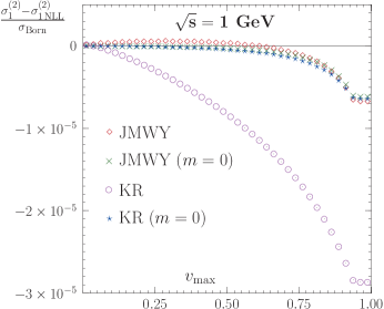
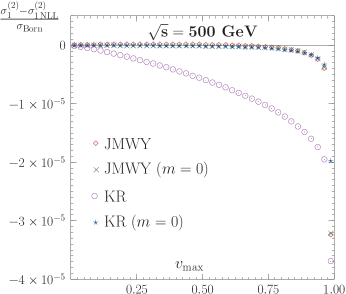
Figure 1: Differences between the exact and massless NLL results for the virtual correction to single photon ISR, both with and without mass corrections, in a ${\cal KK}$MC run of $10^{8}$ events. Results are shown for two different energy scales, $\sqrt{s}=$ 1 GeV and 500 GeV. JMWY is the expression of Ref. [1] and KR is the expression of Ref. [3], and $v_{\max}$ is the limit on the radiated photon energy, relative to the beam energy.

Detailed numerical comparisons[11, 14, 15] have been made using the ${\cal KK}$MC, both at 1 GeV and 500 GeV, corresponding to typical energies for B factories and the ILC, respectively. Since the massless NLL limits are known to agree, we have subtracted the NLL limit (Eq. 4) in each case, and plotted the remaining contribution, both with and without explicit mass terms. The results of MC runs for $10^{8}$ events are shown in Fig. 1, normalized to the Born cross section.

The plots show that the massless results agree to within $10^{-6}$ for all but the last bin of the 500 GeV run. The main difference is evident in the mass corrections. The maximum difference between the integrated cross sections is found to be $2.2\times 10^{-5}$ at 1 GeV and $1.6\times 10^{-5}$ at 500 GeV, in units of the Born cross section. While this is an excellent level of agreement, it is clear that there is some disagreement in the mass corrections, which are responsible for almost the entire difference. It would be desirable to understand the origin of this difference more completely.

References

- [1] S. Jadach, M. Melles, B.F.L. Ward and S.A. Yost, Phys. Rev. D65, 073030 (2002).
- [2] G. Rodrigo, A. Gehrmann-De Ridder, M. Guilesaume, J.H. Kühn, Eur. Phys. J. C22, 81 (2001)
- [3] J.H. Kühn and G. Rodrigo, Eur. Phys. J. C25, 215 (2002).
- [4] R. Kleiss and W.J. Stirling, Nucl. Phys. B262, 235 (1985); Phys. Lett. B179, 159 (1986).
- [5] F.A. Berends, P. De Causmaecker, R. Gastmans, R. Kleiss, W. Troost and T.T. Wu, Nucl. Phys. B264, 243 (1986); ibid., 265.
- [6] Z. Xu, D.-H. Zhang and L. Chang, Nucl. Phys. B291, 392 (1987).
- [7] J.A.M. Vermaseren, Symbolic Manipulation with FORM (Computer Algebra Netherlands, Amsterdam, 1991).
- [8] G.J. van Oldenbourgh and J.A.M. Vermaseren; Zeit. Phys. C46, 425 (1990); G.J. van Oldenbourgh, FF, a package to evaluate one-loop Feynman diagrams (NIKHEF-H/90-15, 1990).
- [9] S. Jadach, B.F.L. Ward, and Z. Wa̧s, Phys. Rev. D63, 113009 (2001); Comput. Phys. Commun. 130, 260 (2000).
- [10] S.A. Yost, C. Glosser, S. Jadach and B.F.L. Ward, Linear Collider Workshop 2004, Paris, hep-ph/0409041.
- [11] S. Jadach, B.F.L. Ward and S.A. Yost, Phys. Rev. D73, 073001 (2006).
- [12] F.A. Berends, R. Kleiss, P. De Causmaecker, R. Gastmans, W. Troost, T.T. Wu, Nucl. Phys. B206, 61 (1982).
- [13] S.A. Yost, C. Glosser, S. Jadach, B.F.L. Ward, in ICHEP 2004: Proceedings of the 32nd International Conference on High Energy Physics, Beijing (World Scientific, Singapore, 2005), 478. hep-ph/0410238.
- [14] S.A. Yost, S. Jadach, and B.F.L. Ward, Acta Phys. Polon. B36, 2379 (2005).
- [15] C. Glosser, S. Jadach, B.F.L. Ward and S.A. Yost, Phys. Lett. B605, 123 (2005).