Toward the AdS/CFT gravity dual for High Energy Collisions:
I.Falling into the AdS

Abstract

In the context of the AdS/CFT correspondence we discuss the gravity dual of a high energy collision in a strongly coupled ${\cal N}=4$ SYM gauge theory. We suggest a setting in which two colliding objects are made of non-dynamical heavy quarks and antiquarks, which allows to treat the process in classical string approximation. Collision “debris” consist of closed as well as open strings. If the latter have ends on two outgoing charges, they are being “stretched” along the collision axes. We discuss motion in AdS of some simple objects first – massless and massive particles – and then focus on open strings. We study the latter in a considerable detail, concluding that they rapidly become “rectangular” in proper time -spatial rapidity $\tau-y$ coordinates with well separated fragmentation part and a near-free-falling rapidity-independent central part. Assuming that in the collisions of “walls” of charges multiple stretching strings are created, we also consider the motion of a 3d stretching membrane. We then argue that a complete solution can be approximated by two different vacuum solutions of Einstein eqns, with matter membrane separating them. We identify one of this solution with Janik-Peschanski stretching black hole solution, and show that all objects approach its (retreating) horizon in an universal manner.

I Introduction

The AdS/CFT correspondence adscft is a duality of the conformal (CFT) $\cal N$=4 supersymmetric Yang-Mills theory and string theory in 5d Anti-de-Sitter space ($AdS_{5}$). Multiple papers use this fascinating theoretical tool, in a regime in which the gauge theory is in a strong coupling regime while string part is in weak coupling – the classical SUGRA regime. The equilibrium finite temperature version of this correspondence, using a black-hole background, was suggested by Witten witten1 . Applications of this version of correspondence to properties of strongly coupled high-T phase of QCD are very actively pursued: we will briefly review those in the next subsection.

The aims of this series of works are however quite different: instead of focusing on equilibrium thermal matter, we hope to develop a gravity dual framework to time-dependent process of high energy collisions. We will not assume equilibration or use macroscopic variables like temperature or hydrodynamic flows: we hope to be able to understand how they naturally appear for collisions of large systems. Instead we focus on motion of strings in $AdS_{5}$ in this work, and, in the second one, on “holograms” which an observer will see in our world – the $AdS_{5}$ boundary – as a function of time.

Since this is the first paper of the series, we decided to start with rather extensive introduction, which describes similar works and summaries our current understanding of the subject.

I.1 Strongly coupled Quark-Gluon Plasma

It is well known that non-perturbative properties of the QCD vacuum phase – confinement and chiral symmetry breaking – are absent above some critical temperature, where matter is in the so called Quark-Gluon Plasma (QGP) phase. Although at high $T$ one naturally expects the QGP to be in a weakly coupled regime, it has been conjectured recently SZ12 that at least at $T=(1-2)T_{c}$ – known as the RHIC domain – it is closer to a ’strongly coupled’ regime (sQGP).

This was a significant “paradigm shift” in the field, and various directions toward the understanding of sQGP constitute a mainstream of the field. Basically there are two competing options: one, based on electric-magnetic duality Liao:2006ry , relates small viscosity and diffusion of sQGP to presence of magnetic monopoles and predicts that it will disappear at $T$ away from critical region. Another – based on AdS/CFT – relates it to “quasiconformal behavior” of QGP at $T>2T_{c}$. A comparison between experimental results from RHIC ($T=(1-2)T_{c}$) with those at LHC (higher $T$) will hopefully shed light on it in near future.

Let us only mention some important developments related to the latter approach, AdS/CFT. In a static finite-$T$ setting with AdS-black hole metric witten1 the study started with classic results on bulk thermodynamics Gubser:1998nz and transport coefficients Policastro:2001yc : those works provided intriguing results. It was shown that while the Equation of State can be quite close to that of weakly coupled plasma, the transport properties can differ from them by orders of magnitude. It is enough to mention that while viscosity to entropy ratio is believed to be limited by the AdS/CFT value from below Kovtun:2004de

$${\eta\over s}>{1\over 4\pi}$$ (1)

recent hydrodynamical studies by three groups visc_hydro have concluded that the experimental data on the so called elliptic flow are better reproduced if this ratio is even smaller than that! (For a possible way out of this puzzle, also based on AdS/CFT, see e.g. Lublinsky:2007mm .)

Then attention focused on high energy jet quenching, with the result that a heavy quark pulls a string, with specific and calculable shape. The AdS/CFT result for the drag force jet and heavy quark diffusion CT , turned out to be correctly related by the Einstein relation. For a recent brief summary see e.g. Shu_adv06 : it is sufficient to mention here that all these results seem to be in much better agreement with what is seen phenomenologically in heavy-ion collisions at RHIC than their weak-coupling counterparts.

Further development of the jet quenching problem was related to the question where does the lost energy go?. In a hydrodynamical context it was suggested that the so called “conical flow” conical of matter should develop, induced by a heavy charge moving in a strongly coupled plasma. The “hologram” of the dragging string has been calculated by Princeton and Seattle groups Gubser ; Chesler:2007an : it described the conical flow picture in stunning detail.

I.2 Gravity dual for heavy Ion collisions

The results mentioned above are all equilibrium ones, obtained using static AdS-black hole metric. Although they should be applicable for a macroscopically large and slowly expanding fireball, one may proceed to more demanding issues related with AdS/CFT in time-dependent out-of-equilibrium setting. Those will provide new insights into equilibration issues, explaining when and with what accuracy thermo- and hydrodynamics become applicable.

In AdS/CFT language going from cold vacuum to hot plasma means going from pure AdS (extremal black hole) to black-hole AdS via creation of trapped surface. Therefore the problem to be considered is a kind of gravitational collapse, occuring in gravity-dual as a result of high energy collision.

The quest for black hole formation in collisions has a long history we would not attempt to review here. Let us just mention that it was discussed for “real” gravity at colliders, which may get possible provided it gets strong due to extra dimensions. Black hole production in AdS spaces were discussed both in cosmological brane world models, as well as in AdS/CFT framework from late 90s: we only mention few papers most related to our work. Black hole emerging from collisions were discussed in $AdS_{5}$ background by Horowitz and ItzhakiHorowitz:1999gf , who considered departing black hole. Giddings and KatzGiddings:2000ay have discussed holograms of the falling objects in $AdS_{5}$ background, in cosmological setting (which has some differences with AdS/CFT one in boundary conditions). In Matschull:1998rv a solution for black hole creation from collision of particles was obtained for a simpler case of $AdS_{3}$ background. It was recently further stuided by Kajantie et al. Kajantie:2007bn .

In the context of gravity dual to heavy ion collisions, the problem of black hole formation was discussed by Sin, Shuryak and Zahed SSZ (SSZ below). One specific solution they discussed in the paper was a “hologram” of a departing black hole, corresponding to a spherically symmetric (Big-Bang-like) solution with a decreasing $T$ . SSZ also proposed two other idealized settings, with d-dimensional stretching, corresponding for d=1 to a collision of two infinite thin walls and subsequent “Bjorken” rapidity-independent expansionBj , with 2d and 3d corresponding to cylindrical and spherical relativistic collapsing walls.

Janik and PeschanskiJanik2 (below referred to as JP) have addressed the simplest wall-on-wall collision. In this case the time and longitudinal coordinate $x_{1}$ are naturally substituted by the proper time and spatial rapidity

$$\tau=\sqrt{t^{2}-x_{1}^{2}},\,\,\,y={1\over 2}log({t-x_{1}\over t+x_{1}})$$ (2)

since the rapidity-independent solution depends on only $\tau$. Instead of solving Einstein equations with certain source, describing gravitationally collapsing “debries” of the collision, JP applied an “inverse logic”, extrapolating into the bulk the metric which yield expected hydrodynamical solution at the boundary. JP found an $asymptotic$ (large-time) solution for a “stretching AdS-BH”. As expected, it indeed possesses a horizon moving away from the $AdS$ boundary, as $z_{horizon}\sim\tau^{1/3}$. A very important feature of the leading-order JP solution is entropy conservation: is that while their presumed horizon is stretching in one direction and contracting in others, to the leading order two effects compensate each other and keep the total horizon area constant. We will discuss a bit more this solution and use it in section IV.1.

Further discussion of the subleading (next power of inverse time) terms has been made by Sin and Nakamura SinNak who identified corrections to the JP solution with the viscosity effects. Terms of still higher order have been subsequently studied Heller:2007qt , but eventually Janik et al Benincasa:2007tp concluded that the expansion series are inconsistent beyond the first few orders. Our view is that this is how it should be, and the arising near-horizon singularity indicate that presence of matter term (absent in JP) is inevitable.

Unlike JP et al we will not use any “inverse logic” and will not be looking for the solutions corresponding to pre-determined hydro on the boundary. Instead we will focus on the formation stage, whether black hole is or is not formed, and will $calculate$ the (time-dependent) stress tensor on the boundary, whether it is a hydro-type on not.

I.3 Hadron collisions in QCD, the Lund model and the “Color Glass”

Rather early in development of QCD, when the notion of confinement and electric flux tubes – known also as the QCD strings – were invented in 1970’s, B.Andersen and collaborators Andersson:1983ia developed what gets to be known as the Lund model of hadronic collisions. Its main idea is that during short time of passage of one hadron through another, the strings can get reconnected, and therefore with certain probability some strings become connected to color charges in two different hadrons. Those strings get stretched longitudinally and then break up into parts, making secondary mesons and (with smaller probability) baryons. Many variants of string-based models were developed, and some descendants –e.g. PYTHIA – remain widely “event generators” till today.

If there are several string stretched, it is usually assumed that both their interaction and influence on breaking is negligible.

However if one either considers very high energy collisions, when a single hadron should be viewed as being made of many color charges (partons), or heavy ion collision, a different asymptotic picture has been proposed. McLerran and Venugopalan McLerran:1993ni argued that instead of multiple string the fields produced should be considered as classical gauge fields –known as Color Glass model – and their subsequent evolution be derived from solution of classical Yang-Mills equation RAJU . They suggested this regime is true at very high parton density, when the effective coupling is weak. Accepting the Color Glass picture as a correct asymptotic for very high parton density and large saturation scale $Q_{s}\rightarrow\infty$, one still wanders what should happen in the case of intermediate scale $Q_{s}\sim.3-1.5\,GeV$.

Recent developments of the so called AdS/QCD proposed a view that this interval of scales in QCD constitute a “strong coupling window”. In particular, Brodsky and Teramond Brodsky:2007vk have argued that the power scaling observed for large number of exclusive processes is not due to perturbative QCD (as suggested originally in 1970’s) but to a strong coupling regime with near-constant coupling (quasi-conformal regime). Polchinski and Strassler Polchinski:2001tt have shown that in spite of exponential string amplitudes one does get power laws scaling for exclusive processes, due to convolution (integration over the $z$ variable) with the power tails of hadronic wave functions. One of us proposed a scenario mydomain for AdS/QCD in which there are two domains, with weak and strong coupling. The gauge coupling rapidly rises at the “domain wall” associated with instantons. Such approach looks now natural in comparison to what happens in heavy ion/finite T QCD, where we do know that at comparable parton densities the system indeed is in a strong coupling regime.

I.4 The goals of this series of papers

In short, it is to study self-consistently the collision process in AdS/CFT. For hadronic collisions we basically follow QCD-string-inspired (Lund) picture of the collision. While QCD phenomenology focused on “string breaking”, in AdS/CFT setting we will have instead their “falling” (departure from the boundary) into the IR.

In this paper we will study in detail motion of “debris” – massless and massive particles and open strings, and membranes – in $AdS_{5}$. In the second paper we will calculate the corresponding “holograms” of these objects – the stress tensor of matter created on the boundary. Although “debris” fly away into the 5-th direction, the usual energy and momenta are conserved in our world, and those “holograms” describe a flow of matter outward from the collision point. As we mentioned already, this can be viewed as a strongly-coupled version of Color Glass, put in the realm of $\cal N$=4 SYM theory.

We hope in subsequent works to go beyond the linearized gravity and follow nonlinear effects leading to a gravitational collapse of debris and formation of trapped surfaces. This would be dual to information loss (entropy production) and appearance of equilibration.

Figure 1: Schematic view of the collision setting. The classical heavy charges move along directions $x_{\pm}$ and collide at the origin. String snapping leads to longitudinally stretched strings (wide black line) which are also extended into the 5-th coordinate $r$ toward the AdS center at $r=0$. The heavy charges move on the plane $r=\infty$

II The setting

One important suggestion made by SSZ is that heavy ion collisions posses “some internal high momentum scale”, usually called $Q_{saturation}$, related to high density of color charges in boosted heavy ions. In order to model it more simply, we now propose substitute energetic light quarks by heavy ones, with the mass $M_{Q}$ of heavy fundamental quarks $Q$ introduced into AdS/CFT via $D_{7}$ braneKarch:2002sh . As soon as $M_{Q}$ is at the scale of $Q_{saturation}$, it makes little dynamical difference: but in the AdS/CFT language treatment of heavy quarks is simpler, as they are sources of classical strings. (This simplifying feature has been put to heavy use in treatment of the heavy quark jet quenching jet .)

We will further assume that heavy quarks have no dynamics of their own, as they are moving along straight lines

$$x_{\pm}=x_{1}\pm vt$$ (3)

with constant velocity $v$, both before and after the collisions, see Fig.1. If so, there is no conventional gluonic radiation on the brane or gravitational radiation from them in the bulk, as there is no acceleration.

The dynamical objects we will focus on are classical strings, ending at these heavy quarks and propagating in the bulk (for metrics changing from AdS to JP-like one). We will study which solutions exist as a function of collision rapidity and whether they are stable or not: we will conclude that at sufficiently large $v>v_{c}$ these strings basically go into free fall toward the AdS center.

The next step is to consider not a single pair of charges (a single stretching string), but many. One limit is a pair of colliding “walls of matter”, containing multiple heavy quarks. For simplicity, think of these two walls as CP mirror images of each other, made of colorless “dipoles”. “Snapping” of their string at the collision leads to multiple strings, all of which being stretched longitudinally.

We then argue that many such strings combined could be considered as a thin singular sheet of matter, referred to below as “membrane”. (Note an important distinction between a membrane and a “true brane”: since the former has only energy-momentum but lacks the RR charges and consequent Coulomb repulsion, it cannot “levitate” like branes, and simply falls under gravity.)

It has been shown by Israel Israel how a gravitational collapse of a thin layer of matter can be described via two different discontinuous $vacuum$ solutions of the Einstein equation without matter ($T_{\mu\nu}=0$). Self-consistency of the solution is then reached by fulfilling covariant junction conditions, resulting in membrane equation of motion.

The issue of self-consistency will not be addressed in this work: we will discuss below falling of various objects – particles and open strings, as well as 3+1 membranes – ignoring for now the effect of their own weight on the metric. The proposed evolution of the system is explained schematically in Fig2. Part (a) of it shows some snapshots of this surface, at some early time and then at a later stage. The horizontal direction is the collision direction $x_{1}$ while the one along the circles represent any of the two other transverse directions $x_{2},x_{3}$ (on which no dependence is expected). The radial direction $r$ in part (b) is the 5-th AdS radial direction, a distance from the AdS center. Since the “membrane” is being stretched in $x_{1}$ (linearly in time), it has to retreat in $r$ and become a thinner cylinder, just as a stretching soap film will do in a similar setting.

At this point we would like to emphasize a close analogy, as well as differences, with the jet quenching problem. One studied first a single falling string governed by simple Nambu-Goto action and the overall metric. The complicated picture of matter flow is then recovered using weak (linearized) gravity. One difference is that in a jet quenching problem the string is stationary (in the charge frame) while in our case it is not. Furthermore, we will discuss also multiple strings, which may form another singular object – the $membrane$. Also the metric in our problem is first considered to be just AdS, but eventually it will be non-trivially affected by the membrane’s own weight. If so, one should no longer use the linearized gravity but solve Einstein equations in its full nonlinear form.

Needless to say, this is a very difficult task, amenable to analytic treatment only if some drastic simplifications are made. A scenario outlined in Fig2(a) would have metric dependent on 3 variables: time, longitudinal direction and the AdS radial one, $t,x_{1},r$. We thus propose a further simplification of the problem: changing variables to proper time and spatial rapidity (2) we would look for $y$-independent solutions, corresponding to purely cylindrical part of the membrane in the middle of Fig2(a), ignoring the curved “fragmentation” regions. With only two variables, $\tau,r$ one has a problem of similar level of complexity as the one addressed by Israel, for a spherical gravitational collapse.

Further clarification of the proposed scenario is shown in Fig.2(b), displaying a trajectory of the membrane $r(\tau)$. During the first stage of the process the “debris” of a collision in a bulk – the particles and open strings – are accelerated by the AdS gravity and fall into the 5-th dimension till they reach the relativistic velocity $v\approx 1$ (stage 2)). If there be only one object falling, its gravity being negligible compared to overall gravity of the $N$ branes at the AdS center and they would simply continue their relativistic fall. However large number of them have enough mass to create a horizon which suddenly slows down the membrane (as a distance observer sees it ): at stage 3 the membrane is trailing the receding horizon (the dashed line).

If we would discuss pure AdS/CFT theory this would be the end of the story: but in other more QCD-like setting one can have an additional potential which will stop membrane because of existence of a stationary “deconfinement” horizon. If so, the system reaches a “mixed phase” era with stationary horizon and fixed $T$, similar to static fireball discussed by Aharoni et al Aharoni except that in our setting the longitudinal stretching continues.

The trajectory of the collapsing matter sheet should be such as to provide a consistent solution to Einstein equations, combining the JP-like vacuum solution outside the falling sheet, with the “stretching AdS” inside it.

Figure 2: (a=upper) Two snapshot of the membrane shapes, at different time moments. See text for explanation of the coordinates. (b=lower)Schematic view of the four periods in gravity dual solution in which falling objects are (1) accelerated into the 5-th dimension $r$ till they reach a relativistic velocity $v\approx 1$, then (2) continue their relativistic fall till (3) breaking near the retreating horizon.

The paper is structured as follows. In the next section we solve equation of motion for different objects falling in AdS. We start with massless and massive particles in subsection III.1.

The main part of this work is study of the open strings, being stretched between two departing charges. We derive analytically the so called $scaling$ (factorisable) solution in section III.2. Similar solutions have been used previously in connection to anomalous dimensions of “kinks”. New part is discussion of the limits for its existence and stability.

We then find more general non-factorisable solutions in section III.3 which can only be obtained numerically. We find that in proper time -spatial rapidity coordinates $\tau,y$ we use those basically becomes “rectangular” , with a nearly free-falling rapidity-independent part. We conclude this section with results for falling membranes. The next section starts with an introduction to the issue of “stretching black holes” in section IV.1, and concludes with section IV.2 in which we show that all objects considered above are approaching the (retreating) horizon in a very universal fashion. We conclude with some discussion and outlook in section V.

In the second paper of the series we will calculate back reaction of gravity, by solving linearized Einstein equations and obtaining stress tensor on the boundary (“holograms”) for some of these falling objects.

III Objects falling in $AdS_{5}$

The collisions creates a lot of “debris” in form of various excitations. Since we would like to follow the collision in the bulk, we naturally have to think of them in terms of string theory. Thus there are the following types of objects: (i) massless and massive particles; (ii) open strings, with ends at the receding walls; (iii) membrane. The “open string” category is naturally split into “mesons” with both ends on the $same$ wall, and “stretched strings”, with both ends attached to different walls and moving in the opposite direction. We will consider a set of multiple strings copied many times in transverse dimensions $x_{2},x_{3}$ as a 3-d membrane. The validity of this approximation will be explained later.

III.1 Falling particles

As is usually done in this kind of problems, the AdS radius is inverted, so that a coordinate $z=1/r$ is used instead of $r$. The AdS boundary is thus at $z=0$ and “falling” objects move away from it toward infinity. The $AdS_{5}\times S^{5}$ metric in such coordinates is

$$ds^{2}={R^{2}\over z^{2}}(d\vec{x}^{2}-dt^{2}+dz^{2})+R^{2}\,d\Omega_{5}^{2}$$ (4)

where the last term, related to angles of $S^{5}$ is of no importance in this work. We choose to work in $\tau$, $y$ coordinates mentioned above (2). The metric is translated into the following form:

$$ds^{2}={R^{2}\over z^{2}}(-d\tau^{2}+\tau^{2}dy^{2}+dz^{2})$$ (5)

where we ignore the transverse coordinates and the $S_{5}$ part.

One feature of $AdS_{5}$ metric is its boost invariance, the importance of which will be seen later. Let us assume particles move with constant spatial rapidity $y$, so the trajectory can be described by $z(\tau)$. Massless particles move along the geodesics with zero interval $ds^{2}=0$ which in the metric (5) simply means $z=\tau$.

Massive falling objects were already discussed in Danielsson:1998wt , but here we present it in a different form, more closely resembling much more nontrivial ones in the next sections. Using the coordinate time $\tau$ one simply write down the interval as an action for a particle moving in the 5-th direction of

$$S\sim\int d\tau{\sqrt{1-\dot{z}(\tau)^{2}}\over z(\tau)}$$ (6)

where the non-trivial trace of the AdS metric is $z$ in the denominator. This leads to well known EOM

$$\ddot{z}(\tau)={1-\dot{z}(\tau)^{2}\over z(\tau)}$$ (7)

Nonrelativistically, one can neglect $\dot{z}(\tau)$ and think thus about a motion in a logarithmic potential well. Ultrarelativistically, one finds instead that as $\dot{z}(\tau)\rightarrow 1$ the acceleration goes to zero, as needed. Thus, in the standard coordinates, very little seems to happen after the particle reaches ultrarelativistic regime: it runs forever toward $z\rightarrow\infty$ with speed of light. But this is a (well known) illusion due to relativistic time slowing: in its own proper time, the particle continue to accelerate and reaches the AdS center in finite proper time.

This EOM is easily integrated yielding

$$z(\tau)=\sqrt{\tau^{2}+v_{0}z_{0}\tau+z_{0}^{2}}$$ (8)

III.2 Falling open strings: the scaling solution

After this little warm-up, let us consider motion of the open strings. Its action is given by Nambu-Goto, and if one ignores two transverse coordinates $x_{2},x_{3}$ and uses as two internal coordinates the $t,x$ (time and longitudinal coordinate) the string is described by by one function of two variables $z(x,t)$. The corresponding string action is then

$$S=-{R^{2}\over 2\pi\alpha^{\prime}}\int dt\int{dx\over z^{2}}\sqrt{1+({\partial z\over\partial x})^{2}-({\partial z\over\partial t})^{2}}$$ (9)

Note that only one term, the time derivative, is different from long-used static action used in MALDA2_REY for static calculation of the inter-charge potential. The boundary conditions would be $z=0$ at two rays $x=\pm vt$, the world lines of the heavy quarks.(The boost invariance of the $AdS_{5}$ metric allows us to work in a frame where the open string endpoints move with opposite velocities)

Translating into the $\tau,y$ language, the boundary conditions are now determined at fixed $y=\pm Y$ where $v=tanhY$ and $Y$ is the rapidity of the heavy quarks (colliding walls). by doing so, we transfer time dependence from the boundary conditions into the equations themselves. The corresponding action is now

$$S=-{R^{2}\over 2\pi\alpha^{\prime}}\int{\tau d\tau dy\over z^{2}}\sqrt{1-\left({\frac{\partial z}{\partial\tau}}\right)^{2}+{\frac{\left({\frac{\partial z}{\partial y}}\right)^{2}}{{\tau}^{2}}}}$$ (10)

Before solving the corresponding equation in full, we will first discuss “scaling” solutions in the separable form

$$z(\tau,y)={\tau\over f(y)}$$ (11)

suggested by conformal properties of the theory. Such solutions were known in literature Gross_Makeenko , in Euclidean context, they were used for AdS/CFT calculation of the anomalous dimensions of “kinks” on the Wilson lines (of which our produced pair of charges is one).

The scaling ansatz leads to a simple action

$$S=-{R^{2}\over 2\pi\alpha^{\prime}}\int{d\tau dy\over\tau}\sqrt{f^{\prime 2}+f^{4}-f^{2}}$$ (12)

Using the fact that $y$ does not appear in the action, there is a conserved “energy”

$${V\over\sqrt{f^{\prime 2}+V}}=E$$ (13)

with the “potential” $V=f^{4}-f^{2}$, and thus the derivative of the function $f$ can be readily obtained

$$f^{\prime}={\sqrt{V(V-E^{2})}\over E}$$ (14)

Note that the function $f$ decreases from infinity on the boundaries to its lowest value at the middle of the string which we will call $f_{0}$, so $f>f_{0}$. At $f=f_{0}$ the derivative vanishes, so (14) provides also a simple equation $f_{0}^{4}-f_{0}^{2}-E^{2}=0$ relating $E$ to $f_{0}$.

Integration of (14) gives the following solution

$$y=f_{0}\sqrt{\frac{f_{0}^{2}-1}{2f_{0}^{2}-1}}{\it F}\left(\sqrt{{\frac{{f}^{2}-{f_{0}^{2}}}{{f}^{2}-1}}},\frac{f_{0}}{\sqrt{2f_{0}^{2}-1}}\right)$$

$$-\frac{1}{f_{0}}\sqrt{\frac{\left(f_{0}^{2}-1\right)^{3}}{\left(2f_{0}^{2}-1\right)}}{\it\Pi}\left(\sqrt{{\frac{{f}^{2}-{f_{0}^{2}}}{{f}^{2}-1}}},{1\over{f_{0}^{2}}},\frac{f_{0}}{\sqrt{2f_{0}^{2}-1}}\right)$$ (15)

where ${\it F}$ and ${\it\Pi}$ are elliptic integral of the first and the third kind. $f_{0}^{2}$ depends on collision rapidity $Y=arctanh(v)$ via the boundary condition at $f(Y)=\infty$, as shown in Fig. 3.

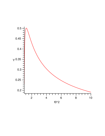
Figure 3: Rapidity of the collision $Y=arctanh(v)$ vs $f_{0}^{2}$. The maximum gives a critical rapidity $Y_{c}$. For $Y<Y_{c}$, two $f_{0}^{2}$ are possible, corresponding two string configurations. For $Y=Y_{c}$ ,only one $f_{0}^{2}$ is possible. The region $Y>Y_{c}$ cannot be reached

The existence of a maximum means that there are no scaling solutions when the rapidity $Y$ is larger than some critical value, while if the quarks move on the boundary slower that the critical rapidity, there are $two$ solutions.

In order to characterize the solutions, it is useful to introduce “effective potential” for two separating quarks for each scaling solution, defined as instantaneous energy $U=\Delta S/\Delta t$, where $\Delta S$ is action given by the area of the string world sheet, $\Delta t$ is the time interval. $U$ needs to be regulated, which is obtained by subtracting the Wilson loop corresponding to two non-interacting moving quarks. In other words, we calculate the subtracted area:

$$S_{reg}=-{R^{2}\over 2\pi\alpha^{\prime}}\int{dt\over t}\int dy\sqrt{f^{\prime 2}+V}-\int_{0}^{\infty}df$$

$$=-{R^{2}\over 2\pi\alpha^{\prime}}\int{dt\over t}\left({\int_{f_{0}}^{\infty}df\sqrt{{\frac{V}{V-E^{2}}}}}-{\int_{0}^{\infty}df}\right)$$ (16)

The second term corresponds to $f^{\prime}=\infty$, precisely the straight string going in $z$ direction, which is AdS solution for a moving quark. Note that we have switched to $t$,$y$ coordinates, which does not change the form of the string action (12). With this prescription, we calculated $U$ for solutions in both branches, which are compared in Fig. 4. The solution with the lower potential has a chance to be the stable one, while the higher potential one (with large $f_{0}$, or longer string) must be metastable.

Let us now comment on the $small$ v limit of the scaling solution. At large separation (realized at late time) the quarks can be considered as quasi-static. At small v, or large $f_{0}^{2}$, the effective potential can be simplified to the following form

$$dS_{reg}/dt=-{R^{2}\over 2\pi\alpha^{\prime}}\int df\left(\sqrt{V\over V-{E}^{2}}-1\right)/t$$

$$=-{R^{2}\over 2\pi\alpha^{\prime}}\left(-0.5991\,\sqrt{f_{0}}-0.1780\,{1\over{f_{0}}}\right)\,{2v\over L}$$ (17)

and relate more simply the velocity and $f_{0}$

$$v={0.5991\over{f_{0}}}-{0.03115\over{f_{0}}^{3}}$$ (18)

Combining (III.2) and (18), we obtain the effective potential for small velocity and large separation to be

$$V=0.2285\,\frac{\left(1+0.6830\,v^{2}\right)\sqrt{g^{2}\,N}}{L}$$ (19)

The coefficient in front (the leading term at $v\rightarrow 0$) coincides with the well known coefficient of static Maldacena potential.

The second term is thus the velocity-dependent “Ampere’s law” $O(v^{2})$ correction to it. We are not aware of any other previous calculation of this term, except for the paper by Zahed and one of us SZ_spin in which, based on resummation of ladder diagrams via Bethe-Salpeter eqn, the result was that the velocity dependence is

$$U(v)/U(v=0)=\sqrt{1-\vec{v}_{1}\vec{v}_{2}}\approx 1+.5v^{2}+...$$ (20)

It is close but not the same.

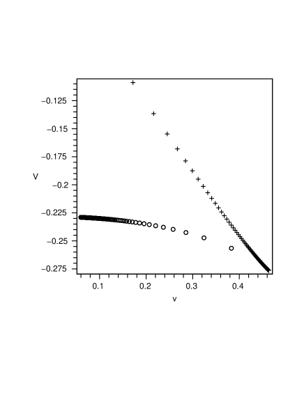
Figure 4: the potential V as a function of v for different branches of solution. circles for large-$f_{0}^{2}$ branch, crosses for small-$f_{0}^{2}$ branch V is plotted in unit of $\sqrt{g^{2}\,N}/L$ The potential from the large $f_{0}^{2}$ branch is lower than that from small $f_{0}^{2}$ branch

Both branches of the scaling solution was also confirmed by solving the equation numerically, starting from the middle point and scanning all values of $f_{0}$.

The applicability of the scaling solution for a particular $Y$ depends of course not only on availability of a solution, but also on its $stability$ i.e. how does the scaling solution evolve with time($\tau$), given some perturbation at initial time. Denoting scaling solution $g_{s}(y)={1\over{f(y)}}$ and perturbation as

$$z(\tau,y)=\tau g(\tau,y)\hskip 28.45274ptg(\tau,y)=g_{s}(y)+\delta g(\tau,y)$$ (21)

we want to know whether the perturbation will grow or decay with time. The EOM for $g(\tau,y)$

$$-2-{\tau}^{3}g({\frac{\partial g}{\partial\tau}})^{3}+2\tau g({\frac{\partial g}{\partial y}})^{2}{\frac{\partial g}{\partial\tau}}-2\tau g^{2}{\frac{\partial g}{\partial y}}{\frac{\partial^{2}g}{\partial\tau\partial y}}+$$

$${\tau}^{2}g({\frac{\partial g}{\partial y}})^{2}{\frac{\partial^{2}g}{\partial{\tau}^{2}}}+2\tau{\frac{\partial^{2}g}{\partial{y}^{2}}}g^{2}{\frac{\partial g}{\partial\tau}}+{\tau}^{2}{\frac{\partial^{2}g}{\partial{y}^{2}}}g({\frac{\partial g}{\partial\tau}})^{2}-2{\frac{\partial g}{\partial y}}-g^{4}$$

$$-{\frac{\partial^{2}g}{\partial{y}^{2}}}g^{2}+7\tau g{\frac{\partial g}{\partial\tau}}-3\tau g^{3}{\frac{\partial g}{\partial\tau}}-3{\tau}^{2}g^{2}({\frac{\partial g}{\partial\tau}})^{2}+{\tau}^{2}g{\frac{\partial^{2}g}{\partial{\tau}^{2}}}$$

$$+3g^{2}+2{\tau}^{2}({\frac{\partial g}{\partial\tau}})^{2}+{\frac{\partial^{2}g}{\partial{y}^{2}}}g^{3}-2{\tau}^{2}g{\frac{\partial g}{\partial y}}{\frac{\partial g}{\partial\tau}}{\frac{\partial^{2}g}{\partial\tau\partial y}}=0$$ (22)

can be used by plugging (21) in (III.2), and keeping only term linear in $\delta g(\tau,y)$(consider only sufficient small perturbation), we obtain the following linearized EOM for the perturbation:

$$\left[A+B\frac{\partial}{\partial\tau}+C\frac{\partial}{\partial y}+D\frac{\partial^{2}}{\partial\tau\partial y}+E\frac{\partial^{2}}{\partial\tau^{2}}+F\frac{\partial^{2}}{\partial y^{2}}\right]\delta g(\tau,y)$$

$$=0$$ (23)

with

$$A=g_{s}^{\prime\prime}g_{s}^{2}+6g_{s}-4g_{s}^{3}-g_{s}^{\prime\prime}$$

$$B=\tau(2g_{s}g_{s}^{\prime 2}+2g_{s}^{\prime\prime}g_{s}^{2}+7g_{s}-3g_{s}^{3})$$

$$C=-4g_{s}^{\prime}$$

$$D=-\tau(2g_{s}^{2}g_{s}^{\prime})$$

$$E=\tau^{2}(g_{s}g_{s}^{\prime 2}+g_{s})$$

$$F=g_{s}^{3}-g_{s}$$

define $\tilde{\tau}=ln\tau$ as our time, the EOM simplifies to:

$$\left[\tilde{A}+\tilde{B}\frac{\partial}{\partial\tilde{\tau}}+\tilde{C}\frac{\partial}{\partial y}+\tilde{D}\frac{\partial^{2}}{\partial\tilde{\tau}\partial y}+\tilde{E}\frac{\partial^{2}}{\partial\tilde{\tau}^{2}}+\tilde{F}\frac{\partial^{2}}{\partial y^{2}}\right]\delta g(\tau,y)$$

$$=0$$ (25)

with

$$\tilde{A}=A,\tilde{B}=B-E,\tilde{C}=C,\tilde{D}=D,\tilde{E}=E,\tilde{F}=F$$ (26)

(To make it easier to get all these functions one can approximate scaling solution $g_{s}(y)$ with some parameterizations: we found that $({\frac{g_{s}}{g_{s}(0)}})^{3}+({\frac{y}{Y}})^{n}=1$ fits all the scaling solution very well.)

We need to seek eigenfunction $\delta g(\tau,y)=e^{\lambda\tilde{\tau}}\psi(y)$ satisfying (III.2) and boundary condition $\psi(y=\pm Y)=0$ In general, out of many eigenvalues $\lambda$ we should be interested in those with positive real part, which will allow us to conclude when the solution is unstable.

The eigenfunction results in the following EOM:

$$\left[C_{0}+C_{1}\frac{\partial}{\partial y}+C_{2}\frac{\partial^{2}}{\partial y^{2}}\right]\psi(y)=0$$ (27)

with

$$C_{0}=\lambda^{2}g_{s}(g_{s}^{\prime 2}+1)+\lambda(g_{s}g_{s}^{\prime 2}+6g_{s}+2g_{s}^{2}g_{s}^{\prime\prime}-3g_{s}^{3})$$

$$+3g_{s}^{\prime\prime}g_{s}^{2}+6g_{s}-4g_{s}^{3}-g_{s}^{\prime\prime}$$

$$C_{1}=-2g_{s}^{\prime}(\lambda g_{s}^{2}+2)$$

$$C_{2}=g_{s}(g_{s}^{2}-1)$$

Due to the symmetry $y\leftrightarrow-y$ of the problem, we can solve it in the positive-$y$ region, with boundary condition $\psi(Y)=0$,$\psi^{\prime}(0)=0$. To solve this Schrodinger-like eqn, we use the iterative method. Starting on one boundary with $\psi^{\prime}(0)=0$,$\psi(0)=1$, the second condition only affects the normalization of $\psi(y)$. With some initial value of $\lambda$, we can obtain the $\psi(Y)$ from the EOM. then we variate the value such that $\psi(Y)$ converge to 0. The resulting $\lambda$ gives the eigenvalue. Without much difficulty, we found the following set of eigenvalue for different $Y$, shown in Table.1. We also plot the eigenvalue $\lambda$ in the complex plane Fig.5. The evolution trend of this set of eigenvalues suggests that the transition from stable to unstable occurs at $Y_{m}$ inside .22-.27 interval, which is way below the critical value $Y\sim.5$ above which there were no scaling solutions at all. This shows that we essentially lose the scaling solution to instability for $Y>Y_{m}$: we were not able to tighten this limits any further.

Table 1: one set of eigenvalue for different rapidity

$\lambda(10^{-2})$	4.2+94.8i	3.3+126.7i	2.8+157.5i	2.0+188.5i
$Y$	0.48	0.45	0.42	0.40
$\lambda(10^{-2})$	1.2+222.1i	0.78+265.7i	0.38+299.5i	0.12+346.4i
$Y$	0.37	0.33	0.30	0.27
$\lambda(10^{-2})$	-0.27+404.2i	-0.63+492.9i	-0.80+569.8i
$Y$	0.24	0.21	0.18

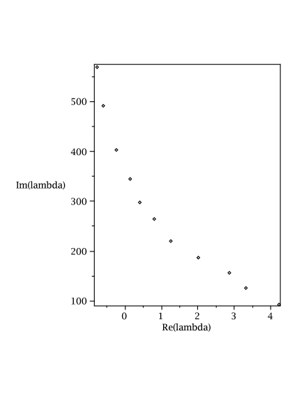
Figure 5: The evolution of eigenvalue $\lambda$ from Y=0.48 to 0.18 in the complex plane

In summary, the scaling solution exist only for sufficiently small rapidities $Y<Y_{c}\sim 0.5$. Furthermore, we were able to verify that it is classically unstable already for $Y>Y_{m}\approx 1/4$. Therefore solutions other than the scaling one is need for large rapidity, which is more important for our purpose.

III.3 Falling strings: the non-scaling solutions

In this section we study generic solutions outside the scaling ansatz. But before we do so, let us explain qualitatively why such solution must fail as the rapidity of the collision grows. The scaling solution, in which $\tau$ and $y$ dependences factorize, means that one tries to enforce a particular stable profile to a string. But as the rapidity gap $2Y$ between the walls grows, we so-to-say try to build wider and wider “suspension bridge” out of the string: it is going to break under its weight at some point.

We again use $z(\tau,y)=\tau g(\tau,y)$ and EOM (III.2). The boundary condition is $g(\tau,y=\pm Y)=0$. Due to the symmetry of the problem, it is sufficient to solve the dynamics of half of the string, with initial condition $g(\tau,Y)=0$ and $\frac{\partial g}{\partial y}(\tau,0)=0$.

However there are two potential problems in (III.2). (i)the $y$ derivative diverges on the boundary. (ii)the PDE is highly nonlinear and will show self-focusing of energy at certain “corners”, as we will see. These make it difficult to obtain a well-behaved numerical solution , and to improve the performance of Maple PDE solver we used function $h(\tau,y)=g(\tau,y)^{n}$ as dynamical variable, with properly chosen integer power $n$ so that the $y$ derivative is finite on the boundary.

Fig.6 shows the dynamics of the string with $Y=0.6$. We start from the initial condition $({g(1,y)\over 0.88})^{3}+({y\over Y})^{3}=1$ and $\frac{\partial g}{\partial\tau}(1,y)=0$. We choose the initial time $\tau=1$ to avoid the singularity at $\tau=0$. $n=6$ is used in solving the PDE. As time grows, the string profile approach a rectangular shape with sharper and sharper turn at the “corners”. Based on the numerical solution, we infer that in the $\tau,y$ coordinates, any point of the string other than the boundary will ultimately become free falling when time is sufficient large. This can be supported by the following qualitative argument. Any tiny piece of string experiences the AdS effective gravity and the drag from its neighbors. Since in the non-scaling solution, the whole string keeps falling, it is natural to expect any point of the string approach the speed of light asymptotically, end up with a rectangular profile. Therefore, we conclude the edge of the profile is not important asymptotically. It can be well approximated by a flat profile in $y$, which will be studied in the next section.

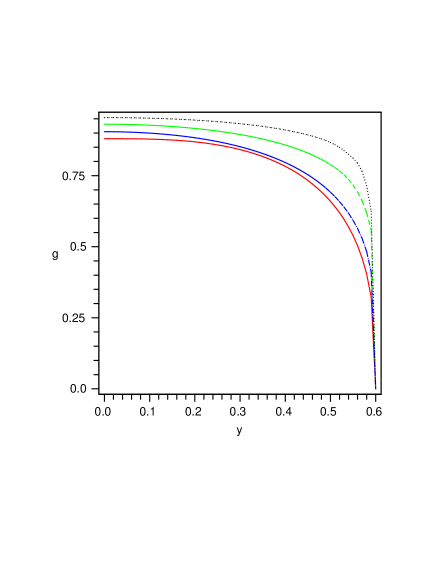
Figure 6: The dynamics of the string(half) $g(\tau,y)$ with $y=0.6$. The profiles from the innermost to the outermost correspond to $\tau=1$(solid red),$\tau=2$(dotted blue),$\tau=4$(dashed green), $\tau=8$(dot-dashed black).

III.4 Falling strings and membrane in $AdS_{5}$

The falling string can be considered as a solution at the center of the generic case considered above in the large rapidity limit of the ends $Y\rightarrow\infty$. which makes $z$ $y$-independent. Ignoring all derivatives over $y$ in the EOM above one gets an ODE problem with the following eqn:

$$-2\,\tau+{\dot{z}}\,z-{{\dot{z}}}^{3}z+\tau\,{\ddot{z}}\,z+2\,{{\dot{z}}}^{2}\tau=0$$ (28)

which is similar but not identical to that of a falling massive object (7): the difference comes from dimensionality of the object: $1/z^{2}$ in the action (instead of $1/z$), because the string action is a 2-dimensional integral. It is now explicitly depending on $\tau$: there is no integral of motion but one can straightforwardly solve the EOM for different initial conditions numerically. We found at large $\tau$, $g$ tends to 1. Therefore we show in this extreme case that the asymptotic solution is again $z\sim\tau$

Summarizing the falling of all string objects, they have a universal asymptotic behavior $z\sim\tau$. Therefore we may model the falling particles/open strings by a membrane, which is made of multiple strings and is flat in $x_{2}$, $x_{3}$ and $y$ coordinates

The coefficient in its DBI action, the membrane tension, is now proportional to the density of charges in the colliding walls, and thus can be very large. This fact would mean that the membrane should eventually be considered heavy enough, so that its weight would affect the metric itself. Since in this work we would not attempt to solve this problem yet, we treat the membrane as a test body falling in external AdS metric. In this case the value of its tension does not matter, and the action is very similar to Nambu-Goto string action except of the different power of $z$ (now $1/z^{4}$)

$$S\sim\int\tau d\tau dydx_{2}dx_{3}{\sqrt{1-({\partial z\over\partial\tau})^{2}}\over z^{4}}$$ (29)

We parametrize the membrane with $\tau$,$y$,$x_{2}$,$x_{3}$, and z-coordinate is a function of $\tau$ only, $z=z(\tau)$. The EOM is readily obtained, it is similar to the $y$-independent string case (coefficients 2 change to 4 in two terms):

$${\dot{z}}z-{\dot{z}}^{3}z+4\tau{\dot{z}}^{2}+\tau{\ddot{z}}z-4\tau=0$$ (30)

Its asymptotic solution is again $z\sim\tau$.

IV Near-horizon “braking”

IV.1 Stretching black holes

The JP solution we will now discuss addresses the first case, d=1. The main feature of the JP solution is that these two variables enter the metric via one specific combination

$$v={z\over\tau^{\gamma}}$$ (31)

which simplifies Einstein’s eqns and leads to a solution. JP have found that only for one particular power $\gamma=1/3$ there is no singularity at the horizon in one of the invariants – the square of the 4-index Riemann curvature, and argued that thus this solution should be preferred on this ground.

However it is not clear what the physical meaning and significance of this singularity may be, in general. Furthermore, in the “membrane scenario” proposed in this work the JP-like metric only extends from the AdS boundary till the falling membrane, while the would-be singularity is in the second domain, where this solution is not supposed to be used at all. It is, so to say, a “mirage behind the mirror”, singular or not does not matter.

There is another reason why this particular power should be selected: only in $\gamma=1/3$ case such that the total area of the horizon (3d object normal to time and z) is time independent: the factor $\tau$ (from stretching $y_{1}$) is canceled by the factor $1/z^{3}$ from contracting $z$. Thus, this stretching solution is area-preserving, and thus potentially dual to the entropy-conserving adiabatically expanding fireball.

The specific form of the JP metric is

$$ds^{2}=-\frac{(1-v^{4}{e_{0}\over 3})^{2}}{(1+v^{4}{e_{0}\over 3})}\frac{d\tau^{2}}{z^{2}}+(1+v^{4}{e_{0}\over 3})\frac{\tau^{2}dy^{2}+dx_{\perp}^{2}}{z^{2}}+\frac{dz^{2}}{z^{2}}$$ (32)

The horizon determined from $g_{\tau\tau}(v)=0$ is at $v_{h}=({3\over e_{0}})^{1/4}$, thus it is moving away from $z=0$ (the AdS boundary) as needed. The 4-th power of $v$ is related to the fact that its expansion near $z=0$ to the 4-th order is responsible for the stress tensor as observed on the boundary, which was tuned to correspond to the Bjorken boost invariant solution of ideal hydrodynamics Bj : the starting point for JP.

This metric provides an asymptotic (large $\tau$) solution to the Einstein eqns

$$R_{\mu\nu}-(R/2)g_{\mu\nu}-6g_{\mu\nu}=\kappa T_{\mu\nu}$$ (33)

After this metric is substituted to the l.h.s. one finds that all terms of the “natural” order of magnitude $O(\tau^{-2/3})$ cancel out, with only the higher order terms remaining. More specifically, we found that only the terms $T_{\mu\nu}\sim 1/\tau^{2}$ are present, with rather compact expressions such as

$$\tau^{2}T_{\tau\tau}=-{4v\over(3+v)^{2}}$$ (34)

$$\tau^{2}T_{zz}=-{4v^{2}\over(3+v)(v-3)^{2}}$$ (35)

$$\tau^{2}T_{yy}=(-4/9){v(4v^{2}-15v-63)\over(v-3)^{3}}$$ (36)

Please note that those terms are not only subleading at large $\tau$ but also are much simpler than all the terms which had canceled out. Also note that there is a significant singularity at the horizon ($v=3$ in these units) in this stress tensor, which is again irrelevant because this metric is not supposed to be used there.

IV.2 Objects approaching the horizon

Before we discuss the JP metric, let us remind the reader how this approach works in the usual black holes with the Schwartzschild metric: it will be needed to emphasize the difference between them.

Massless particle falling radially in the Schwartzschild metric satisfies the $ds^{2}=0$ eqn, which is

$$({dr\over dt})^{2}=(1-{r_{h}\over r})^{2}$$ (37)

leading to exponentially fast “freezeout”,

$$(r-r_{h})\sim exp(-t/r_{h})$$ (38)

The same is also true for other objects, of course.

We use the following rescaled coordinates:

$$z\rightarrow c\,z,\tau\rightarrow c\,\tau,y\rightarrow y,x_{\perp}\rightarrow c\,x_{\perp}$$

with $c=({\frac{3}{e_{0}}})^{\frac{3}{8}}$. The resultant metric is

$$ds^{2}=-\frac{\left(1-{\frac{{z}^{4}}{{\tau}^{4/3}}}\right)^{2}}{1+{\frac{{z}^{4}}{{\tau}^{4/3}}}}\frac{d{\tau}^{2}}{z^{2}}+\left(1+{\frac{{z}^{4}}{{\tau}^{4/3}}}\right)\frac{{\tau}^{2}dy^{2}+dx_{\perp}^{2}}{z^{2}}+\frac{dz^{2}}{z^{2}}$$ (39)

The massless particle moves according to $ds^{2}=0$, which in JP metric is

$$\frac{dz}{d\tau}=\frac{1-{\frac{{z}^{4}}{{\tau}^{4/3}}}}{\sqrt{1+{\frac{{z}^{4}}{{\tau}^{4/3}}}}}$$ (40)

We have assumed that the particle always starts from outside the horizon: $z<\tau^{\frac{1}{3}}$ This EOM is solved numerically for different initial conditions.(From here on, we always use $\tau=10$ as initial time for numerical solution, since the metric (39) is valid asymptoticly $\tau>>1$)

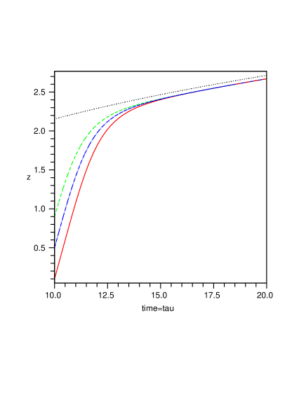
Figure 7: trajectories of massless particles, with initial z coordinates: z(10)=0.1(solid red) z(10)=0.5(dash-dotted blue) z(10)=0.9(dashed green) The horizon is also plotted(dotted black) for comparison. The trajectories of the massless particles approach each other asymptotically, but does not seem to approach the moving horizon.

To obtain the analytical form of the asymptotic behavior, we define:

$$u=\frac{z^{4}}{\tau^{\frac{4}{3}}}$$ (41)

and the EOM becomes

$${\frac{1-u}{\sqrt{1+u}}}=\frac{1}{4}\,{\frac{\dot{u}\,{\tau}^{1/3}}{{u}^{3/4}}}+\frac{1}{3}\,{\frac{{u}^{1/4}}{{\tau}^{2/3}}}$$ (42)

Note $u\rightarrow 1$ as $\tau\rightarrow\infty$. Assuming the second term dominates the first term on the RHS, we obtain the asymptotic form $u=1-\frac{\sqrt{2}}{3}\,\tau^{2/3}$, which confirms our assumption. In terms of $z$ and $\tau$, we have:

$$z=\tau^{1/3}\,\left(1-\frac{1}{6\sqrt{2}}\,\tau^{-2/3}\right)$$ (43)

For massive particle, the action is given by $S=m\int{ds}$. Similarly we focus on the case that particle moves in a trajectory with constant $y$ and $x_{\perp}$: EOM follows from variation on action. Let $z=\tau^{1/3}\,f$, then the function $f$ needs to satisfy the following eqn:

$$-27{\tau}^{2}{f}^{16}{{\dot{f}}}^{2}-6\tau{f}^{17}{\dot{f}}+18{\tau}^{2}{f}^{8}{{\dot{f}}}^{2}-108{\tau}^{2}{f}^{12}{{\dot{f}}}^{2}-6{f}^{14}$$

$$+4{f}^{10}+54\tau{f}^{5}{\dot{f}}-54\tau{f}^{13}{\dot{f}}+12\tau f{\dot{f}}+108{\tau}^{2}{f}^{4}{{\dot{f}}}^{2}$$

$$-6\tau{f}^{9}{\dot{f}}+6{f}^{6}-3{f}^{18}+9{\tau}^{2}{f}^{17}{\ddot{f}}+9{\tau}^{2}f{\ddot{f}}-9{\tau}^{4/3}$$

$$-18{\tau}^{2}{f}^{9}{\ddot{f}}-126{\tau}^{4/3}{f}^{12}+9{\tau}^{4/3}{f}^{20}+27{\tau}^{4/3}{f}^{16}$$

$$-27{\tau}^{4/3}{f}^{4}+126{\tau}^{4/3}{f}^{8}-{f}^{2}+9{\tau}^{2}{{\dot{f}}}^{2}=0$$ (44)

It is again solved numerically, with initial conditions satisfying $z_{0}<\tau_{0}^{1/3}$ and $\dot{z}(\tau_{0})<\frac{1-{\frac{{z_{0}}^{4}}{{\tau_{0}}^{4/3}}}}{\sqrt{1+{\frac{{z_{0}}^{4}}{{\tau_{0}}^{4/3}}}}}$. Note that free falling massive object will move with speed of light asymptotically. We expect (43) to be the asymptotic solution. By plugging (43) in (IV.2), we get the RHS: ${8\over 3}\tau^{-4/3}$, which tends to zero as $\tau$ grows

Furthermore, we compare numerical solution with the asymptotic solution in Fig.8. The two solutions agree well at large $\tau$. This confirms (43) is the correct asymptotic solution.

Figure 8: trajectory of massive particles starting with $f=0.8$ and $\dot{f}=0$.(solid red) at $\tau=10$. The trajectory is indistinguishable from the asymptotic solution(dashed black) at $\tau\sim 15$

To study the falling string, we first parameterize the string by $z=z(\tau,y)$. Instead of solving it this form. We recall our experience with non-scaling solution in AdS space. At large enough $\tau$, the edge of the string will be less important, with most part of the string falling freely. Therefore we ignore the y dependence of z: $z=z(\tau)$

Defining $f=\frac{z}{\tau^{1/3}}$, The EOM follows straightforwardly from the Nambu-Goto action with the metric (39). It is a quite lengthy expression, which we choose not to show here.

We expect the same asymptotic solution (43). By plugging (43) in the EOM, we get the RHS: $-\frac{95\sqrt{2}}{12}\tau^{-2/3}$, which tends to zero as $\tau$ grows. Fig.9 compares numerical solution with the asymptotic solution, which confirms it is the correct asymptotic solution.

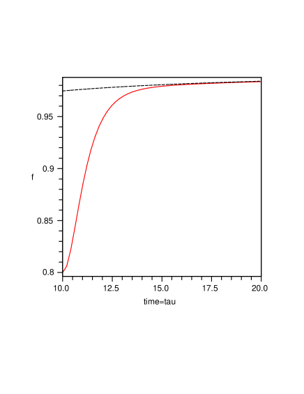
Figure 9: trajectory of string with initial condition $f=0.8$ and $\dot{f}=0$(solid red) at $\tau=10$. The trajectory is indistinguishable from the asymptotic solution(dashed black) at $\tau\sim 15$

Now we proceed to our final case, a $membrane$ falling in JP metric. Let $z(\tau,y,x_{2},x_{3})=\tau^{1/3}f(\tau)$: the EOM is again quite lengthy and not shown here.

We have solved it with a number of initial conditions and found that all extra terms are subleading near horizon, so this EOM gives the same asymptotic solution as the other cases, namely $f=1-({1\over{6\sqrt{2}}})\tau^{-2/3}$.

The numerical solutions are displayed in Fig.10, which confirm the asymptotic solution.

Figure 10: trajectory of membrane with initial condition $f=0.8$ and $\dot{f}=0$(solid red) at $\tau=10$. The trajectory is indistinguishable from the asymptotic solution(dashed black) at $\tau\sim 15$

We found that in all cases studied – massless and massive particles, string and membranes – their late time behavior can be approximated by the same asymptotic solution

$$(z-z_{h}(\tau))\sim[-{1\over{6\sqrt{2}}}\tau^{-1/3}+...]$$ (45)

V Summary

This is the first paper of the series, devoted to quantitative formulation of the “gravity dual” to high energy collisions of macroscopically large bodies (heavy ions). In it we have formulated the setting in which the problem is simplified sufficiently to be solvable.

Its central idea is that various “debris” from a collisions, in form of massless and massive particles or “stretching” open strings, all fall toward the AdS center. Although qualitatively such falling may look quite similar, the equations of motion and solutions are different for different objects. The main result of this work is a systematic demonstration of this statement in detail, both for initial time (when the underlying metric is supposed to be close to AdS) and at the late times (when the metric is close to JP solution). As we will see in subsequent papers later, small differences in “falling” leads to quite different “holograms” in form of stress tensor at the boundary.

One possible solution can be to unify all such “debris” as a single massive “membrane”, falling under its own weight. As shown first by Israel Israel long ago, in such case one can greatly simplify the gravitational aspect of the problem, using two different solutions of the sourceless Einstein equations inside both space-time domains, appropriately matched at the hypersurface made by the world-volume of the membrane. Two solutions are subject to “junction conditions” providing new EOM for the membrane itself. We will discuss those issues elsewhere.

Let us now point out few more specific results of this work. In the study of longitudinally stretched strings we have found that “scaling” solutions used previously for determination of “kink”’s anomalous dimensions are not at all adequate in Minkowski time. We found that while for wall rapidity $Y>Y_{max}\approx 1/2$ these solutions are absent, and there are two of them for smaller $Y$. We further studied stability of the solutions and have proven that at least for $Y>Y_{c}\sim 1/4$ they indeed are unstable.

Our main finding for generic non-scaling solutions (which come from numerical solutions of PDEs) is that while at small velocity of stretching there is the so called scaling solution, generically at high stretching one gets instead asymptotic approach to a “rectangular” solution, consisting basically of two near-vertical strings and freely falling horizontal part.

Another result which was not expected is that although all types of objects – massless and massive particles as well as open strings and membranes – approach the JP horizon in the same universal way. Unlike in the textbook case of the Schwartzschild metric, this approach does not happen exponentially but only as a power $\tau^{-2/3}$ of time. Note that this power is the same as appears in subleading terms, ignored by JP at late time. It remains a challenge to find an appropriate vacuum solution to Einstein equation complementing the late-time JP metric.

Acknowledgments We thank Ismail Zahed and San-Jing Sin for multiple discussions. Our work was partially supported by the US-DOE grants DE-FG02-88ER40388 and DE-FG03-97ER4014.s

References

- (1) J. M. Maldacena, Adv. Theor. Math. Phys. 2, 231 (1998) [Int. J. Theor. Phys. 38, 1113 (1999)] [arXiv:hep-th/9711200].
- (2) E.Witten, Adv.Theor.Math.Phys.2,235 (1998), hep-th/9802150.
- (3) E.V.Shuryak, Prog. Part. Nucl. Phys. 53, 273 (2004) [ hep-ph/0312227]. E.V.Shuryak and I. Zahed, hep-ph/0307267, Phys. Rev. C 70, 021901 (2004) Phys. Rev. D69 (2004) 014011. [ hep-th/0308073].
- (4) J. Liao and E. Shuryak, Phys. Rev. C 75, 054907 (2007) [arXiv:hep-ph/0611131].
- (5) S. S. Gubser, I. R. Klebanov and A. A. Tseytlin, Nucl. Phys. B 534, 202 (1998) [arXiv:hep-th/9805156].
- (6) G. Policastro, D. T. Son and A. O. Starinets, Phys. Rev. Lett. 87, 081601 (2001) [arXiv:hep-th/0104066].
- (7) P. Kovtun, D. T. Son and A. O. Starinets, Phys. Rev. Lett. 94, 111601 (2005) [arXiv:hep-th/0405231].
- (8) P. Romatschke and U. Romatschke, “How perfect is the RHIC fluid?,” arXiv:0706.1522 [nucl-th]. H. Song and U. W. Heinz, “Suppression of elliptic flow in a minimally viscous quark-gluon plasma,” arXiv:0709.0742 [nucl-th]. K. Dusling and D. Teaney, “Simulating elliptic flow with viscous hydrodynamics,” arXiv:0710.5932 [nucl-th].
- (9) M. Lublinsky and E. Shuryak, Phys. Rev. C 76, 021901 (2007) [arXiv:0704.1647 [hep-ph]].
- (10) J. Casalderrey-Solana and D. Teaney, Phys. Rev. D 74, 085012 (2006) [arXiv:hep-ph/0605199].
-
(11)
H. Liu, K. Rajagopal, and U. A. Wiedemann,
Phys. Rev. Lett. 97, 182301 (2006)
[arXiv:hep-ph/0605178].
A. Buchel, Phys. Rev. D 74, 046006 (2006) [arXiv:hep-th/0605178].
C. P. Herzog, A. Karch, P. Kovtun, C. Kozcaz, and L. G. Yaffe, JHEP 0607, 013 (2006) [arXiv:hep-th/0605158].
S. S. Gubser, Phys. Rev. D 74, 126005 (2006) [arXiv:hep-th/0605182]. - (12) E. V. Shuryak, “Strongly coupled quark-gluon plasma: The status report,” arXiv:hep-ph/0608177. “Electric-Magnetic Struggle in QGP, Deconfinement and Baryons,” arXiv:0709.2175 [hep-ph].
- (13) J. Casalderrey-Solana, E. V. Shuryak and D. Teaney, “Conical flow induced by quenched QCD jets,” hep-ph/0411315. arXiv:hep-ph/0602183. H. Stoecker, “Collective Flow signals the Quark Gluon Plasma,” Nucl. Phys. A 750, 121 (2005) [arXiv:nucl-th/0406018].
- (14) J. J. Friess, S. S. Gubser and G. Michalogiorgakis, JHEP 0609, 072 (2006) [arXiv:hep-th/0605292].
- (15) P. M. Chesler and L. G. Yaffe, Phys. Rev. Lett. 99, 152001 (2007) [arXiv:0706.0368 [hep-th]].
- (16) H. J. Matschull, Class. Quant. Grav. 16, 1069 (1999) [arXiv:gr-qc/9809087].
- (17) G. T. Horowitz and N. Itzhaki, JHEP 9902, 010 (1999) [arXiv:hep-th/9901012].
- (18) S. B. Giddings and E. Katz, J. Math. Phys. 42, 3082 (2001) [arXiv:hep-th/0009176].
- (19) K. Kajantie, J. Louko and T. Tahkokallio, arXiv:0705.1791 [hep-th].
- (20) E. Shuryak, S. J. Sin and I. Zahed, arXiv:hep-th/0511199.
- (21) J.D. Bjorken, Phys.Rev.D27 (1983) 140.
- (22) R. A. Janik and R. Peschanski, Phys. Rev. D 73, 045013 (2006) arXiv:hep-th/0512162, arXiv:hep-th/0606149.
- (23) S. Nakamura and S. J. Sin, arXiv:hep-th/0607123.
- (24) M. P. Heller and R. A. Janik, Phys. Rev. D 76, 025027 (2007) [arXiv:hep-th/0703243].
- (25) P. Benincasa, A. Buchel, M. P. Heller and R. A. Janik, arXiv:0712.2025 [hep-th].
- (26) B. Andersson, G. Gustafson, G. Ingelman and T. Sjostrand, Phys. Rept. 97, 31 (1983).
- (27) S. J. Brodsky and G. F. de Teramond, arXiv:0709.2072 [hep-ph].
- (28) L. D. McLerran and R. Venugopalan, Phys. Rev. D 49, 2233 (1994) [arXiv:hep-ph/9309289].
- (29) A. Krasnitz, Y. Nara and R. Venugopalan, Nucl. Phys. A 727, 427 (2003) [arXiv:hep-ph/0305112].
- (30) J. Polchinski and M. J. Strassler, Phys. Rev. Lett. 88, 031601 (2002) [arXiv:hep-th/0109174].
- (31) E. Shuryak, A ”Domain Wall” scenario for the AdS/QCD,arXiv:0711.0004
- (32) A. Karch and E. Katz, JHEP 0206, 043 (2002) [arXiv:hep-th/0205236].
- (33) W.Israel, Nuovo Cimento XLIV B,1 (1966)
- (34) O. Aharony, S. Minwalla and T. Wiseman, “Plasma-balls in large N gauge theories and localized black holes,” hep-th/0507219.
- (35) J. M. Maldacena, Phys. Rev. Lett. 80, 4859 (1998) [arXiv:hep-th/9803002]. S. J. Rey and J. T. Yee, Eur. Phys. J. C 22, 379 (2001) [arXiv:hep-th/9803001].
- (36) D. J. Gross, A. Mikhailov and R. Roiban, Annals Phys. 301, 31 (2002) [arXiv:hep-th/0205066]. Y. Makeenko, P. Olesen and G. W. Semenoff, Nucl. Phys. B 748, 170 (2006) [arXiv:hep-th/0602100].
- (37) U. H. Danielsson, E. Keski-Vakkuri and M. Kruczenski, JHEP 9901, 002 (1999) [arXiv:hep-th/9812007].
- (38) E. V. Shuryak and I. Zahed, Phys. Lett. B 608, 258 (2005) [arXiv:hep-th/0310031].