The NNLO non-singlet QCD analysis of parton distributions based on Bernstein polynomials

Abstract:

A non-singlet QCD analysis of the structure function $xF_{3}$ up to NNLO is performed based on the Bernstein polynomials approach. We use recently calculated NNLO anomalous dimension coefficients for the moments of the $xF_{3}$ structure function in $\nu N$ scattering. In the fitting procedure, Bernstein polynomial method is used to construct experimental moments from the $xF_{3}$ data of the CCFR collaboration in the region of $x$ which is inaccessible experimentally. We also consider Bernstein averages to obtain some unknown parameters which exist in the valence quark densities in a wide range of $x$ and $Q^{2}$. The results of valence quark distributions up to NNLO are in good agreement with the available theoretical models. In the analysis we determined the QCD-scale $\Lambda^{\overline{MS}}_{QCD,N_{f}=4}=211$ MeV (LO), $259$ MeV (NLO) and $230$ MeV (NNLO), corresponding to $\alpha_{s}(M_{Z}^{2})=0.1291$ LO, $\alpha_{s}(M_{Z}^{2})=0.1150$ NLO and $\alpha_{s}(M_{Z}^{2})=0.1142$ NNLO. We compare our results for the QCD scale and the $\alpha_{s}(M_{Z}^{2})$ with those obtained from deep inelastic scattering processes.

1 Introduction

The global parton analysis of deep inelastic scattering (DIS) and the related hard scattering data are generally performed at next-to leading order (NLO). Presently the next-to leading order is the standard approximation for most of the important processes in QCD. Analyzing DIS at next-to-next-to-leading order (NNLO) is important as we may be able to investigate the hierarchy LO $\rightarrow$ NLO $\rightarrow$ NNLO for the processes using the most precise available data.

The corresponding one- and two-loop splitting functions have been known for a long time [1-11]. The NNLO corrections should be included in order to arrive at quantitatively reliable predictions for hard processes occurring at present and future high-energy colliders. These corrections are so far known only for the structure functions in the deep-inelastic scattering [12-15], for the Drell-Yan lepton-pair and gauge-boson production in proton–(anti-)proton collisions [16-19], and the related cross sections for Higgs production in the heavy-top-quark approximation [17,20-22].

Recently much effort has been invested in computing NNLO QCD corrections to a wide variety of partonic processes and therefore it is needed to generate parton distributions also at NNLO, so that the theory can be applied in a consistent manner. Analysis on the NNLO cross sections for jet production is under way and it is expected to yield results in the near future, see Ref. [23] and references therein. For the corresponding three-loop splitting functions, on the other hand, only partial results have been obtained up to now, most notably on the lowest six/seven (even or odd) integer-$N$ Mellin moments [24-26].
S. Moch et al. [27] computed the higher order contributions up to three-loop splitting functions governing the evolution of unpolarized non-singlet quark densities in the perturbative QCD.

During the recent years the interest to use CCFR data [28] for $xF_{3}$ structure function in the higher orders, based on the orthogonal polynomial expansion method has increased [29-34].

In this paper we determine the flavor non-singlet parton distribution functions, $xu_{v}(x,Q^{2})$ and $xd_{v}(x,Q^{2})$, using the Bernstein polynomial approach up to the NNLO level. This calculation is possible now, as the non-singlet anomalous dimension coefficients in $N$-Moment space in three loops has already been introduced [27, 35].

The plan of the paper is to give an introduction to the CCFR data in Section 2. In Section 3 we present a brief review of QCD formalism of the non-singlet structure function in three loops. Parametrization of parton densities are written down in Section 4. Section 5 contains a description of the Bernstein polynomial averages to be employed in the fits. Non-singlet quark distributions in the $x$-space are illustrated in Section 6. Section 7 contains a discussion and conclusions.

2 CCFR experimental data

The measurements of the CCFR collaboration provide a precise determination of the non-singlet deep inelastic scattering structure functions of neutrinos and anti-neutrinos on nucleons, $xF_{3}(x,Q^{2})$. Data for $xF_{3}$ in neutrino-nucleon scattering is available from the CCFR collaboration [28]. The data was obtained from the scattering of neutrinos off iron nuclei and the measurements span the ranges $1.26\leq Q^{2}\leq 199.5\;{\rm{GeV}}^{2}$ and $0.015\leq x\leq 0.75$.

The $Q^{2}$-dependence of moments of structure functions can be predicted in perturbative QCD, and fits to data can be used to infer $\alpha_{s}(M_{Z}^{2})$. A difficulty is that there are upper and lower limits on the experimentally accessible range of $x$ at low and high $Q^{2}$, respectively. This is shown in Fig.1 in which we plot the CCFR data for different values of $Q^{2}$. We can see that at the lower range of $Q^{2}$ we are limited to low-$x$ data, and at high $Q^{2}$ we are limited to the high $x$ range.

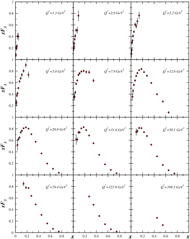
Figure 1: CCFR $xF_{3}$ experimental data as a function of $x$ and for some different values of $Q^{2}$.

In order to reliably evaluate a moment at a particular $Q^{2}$, we require data for the whole range of $x$. In fact for a given value of $Q^{2}$, only a limited number of experimental points, covering a partial range of values of $x$ are available. The method devised to deal with this situation is to take averages of the structure function weighted by suitable polynomials.

Before reconstructing of the structure function from moments, we need to know how the structure function behaves in the missing data region. As we will see in next sections, in the fitting procedure we need to fit the $xF_{3}$ data of the CCFR collaboration. In this regard we can choose the extrapolation method. In this method, we fit $x{F_{3}}(x,{Q^{2}})$ for each fixed value of $Q^{2}$ separately to the phenomenologically convenient expression

$$xF_{3}^{(phen)}(x)={\cal{A}}x^{\cal{B}}(1-x)^{\cal{C}}\;.$$ (1)

This form ensures zero values for ${xF_{3}}$ at $x=0$, and $x=1$. The parameters ${\cal{A}}$, ${\cal{B}}$ and ${\cal{C}}$ are obtained by performing $\chi^{2}$ fitting of Eq. (1) to data for $xF_{3}$. They are $Q^{2}$-dependent quantities, and errors on their values are obtained by performing the fitting with the data for $xF_{3}$ shifted to the two extremes of the error bars.

In Table 1 we have presented the numerical values of $\cal{A},\cal{B}$ and $\cal{C}$ at $Q^{2}=20$, $31.6$, $50.1$, $79.4$, $125.9$ GeV². We have only included data for ${Q}^{2}{\geq}\;20$ GeV², this has the merit of simplifying the analysis by avoiding evolution through flavor thresholds.

Q2(GeV2)	$\mathcal{A}$	$\mathcal{B}$	$\mathcal{C}$
$20$	$4.7425\pm 0.7585$	$0.6356\pm 0.0638$	$3.3756\pm 0.0892$
$31.6$	$5.4735\pm 0.8722$	$0.6936\pm 0.0456$	$3.6595\pm 0.0537$
$50.1$	$5.6795\pm 0.4841$	$0.6977\pm 0.0843$	$3.8390\pm 0.0459$
$79.4$	$4.5076\pm 0.5033$	$0.5666\pm 0.0808$	$3.7574\pm 0.0486$
$125.9$	$7.0775\pm 0.8641$	$0.8186\pm 0.0475$	$4.2456\pm 0.0458$

Table 1: Numerical values of fitting ${\cal{A}},{\cal{B}},{\cal{C}}$ parameters in Eq. (1).

3 QCD formalism

To carry out the analogous analysis at NNLO we need both the relevant splitting functions as well as the coefficient functions. Now not only the deep inelastic coefficient functions are known at NNLO, but also the anomalous dimensions in $N$-Moment space are available at this order [27, 35]. In this section we want to introduce the non-singlet structure function in Mellin moment space up to three loops order.

The structure function $xF_{3}$, associated with the parity-violating weak interaction, represents the momentum density of valence quarks. So in the LO approximation we can write,

$$xF_{3}^{\nu N}=xu_{v}(x)+xd_{v}(x)+2\;xs(x)-2\;xc(x)\;,$$ (2)

$$xF_{3}^{\bar{\nu}N}=xu_{v}(x)+xd_{v}(x)-2\;xs(x)+2\;xc(x)\;,$$

where $u_{v}\equiv u-\bar{u}$ and $d_{v}\equiv d-\bar{d}$ are the proton valence densities. The asymmetry of the $s-c$ doublet results in $xF_{3}^{\nu N}\neq xF_{3}^{\bar{\nu}N}$. The method of extracting CCFR experimental data, extracts the average of the neutrino and anti-neutrino distributions, so that

$$xF_{3}(x)=\frac{xF_{3}^{\nu N}+xF_{3}^{\bar{\nu}N}}{2}=xu_{v}(x)+xd_{v}(x)\;,$$ (3)

here it is obvious that the $xF_{3}(x)$ is related to the combination of valence quark densities.
Let us now define the Mellin moments for the $\nu N$ structure function $xF_{3}(x,Q^{2})$:

$${{\cal{M}}_{3}^{\nu N}(N,Q^{2})}=\int_{0}^{1}x^{N-1}F_{3}(x,Q^{2})dx\;.$$ (4)

The theoretical expression for these moments obey the following renormalization group equation [29]

$$\bigg{(}\mu\frac{\partial}{\partial\mu}+\beta(A_{s})\frac{\partial}{\partial A_{s}}+\gamma_{N}^{NS}(A_{s})\bigg{)}{\cal{M}}(N,Q^{2}/\mu^{2},A_{s}(\mu^{2}))=0\;.$$ (5)

The symbol $A_{s}$ denotes the strong coupling constant normalized to $A_{s}=\alpha_{s}/(4\pi)$ and is governed by the QCD $\beta$-function as

$$\mu\frac{\partial A_{s}}{\partial\mu}=\beta(A_{s})=-2\sum_{i\geq 0}\beta_{i}A_{s}^{i+2}\;.$$ (6)

Eq.(6) is solved in the ${\overline{MS}}$-scheme applying the matching of flavor thresholds at $Q^{2}=m_{c}^{2}$ and $Q^{2}=m_{b}^{2}$ with $m_{c}=1.5$ GeV and $m_{b}=4.5$ GeV as described in [36, 37]. ${\overline{MS}}$-scheme convention introduced in [38] is extended in this way. In order to be able to make a comparison with the other measurements of $\Lambda_{QCD}$ we adopt this prescription. The solution of Eq.(6) in the NNLO is given by

$$A_{s} = \frac{1}{\beta_{0}\ln Q^{2}/\Lambda_{\overline{MS}}^{2}}-\frac{\beta_{1}\ln(\ln Q^{2}/\Lambda_{\overline{MS}}^{2})}{\beta_{0}^{3}(\ln Q^{2}/\Lambda_{\overline{MS}}^{2})^{2}}+$$

$$\frac{1}{\beta_{0}^{5}(\ln Q^{2}/\Lambda_{\overline{MS}}^{2})^{3}}[\beta_{1}^{2}\ln^{2}(\ln Q^{2}/\Lambda_{\overline{MS}}^{2})-\beta_{1}^{2}\ln(\ln Q^{2}/\Lambda_{\overline{MS}}^{2})+\beta_{2}\beta_{0}-\beta_{1}^{2}]\;.$$

Notice that in the above the numerical expressions for $\beta_{0}$, $\beta_{1}$ and $\beta_{2}$ are

$$\beta_{0} = 11-0.6667f\;,$$

$$\beta_{1} = 102-12.6667f\;,$$

$$\beta_{2} = 1428.50-279.611f+6.01852f^{2}\;,$$ (8)

where $f$ denotes the number of active flavors.

In Mellin-$N$ space the evolution equation is solved [32]. The non singlet structure function ${\cal{M}}(N,Q^{2})$ is given by

$${{\cal{M}}(N,Q^{2})}=[1+C^{(1)}(N)A_{s}+C^{(2)}(N)A_{s}^{2}]\;{f^{NS}(N,Q^{2})}\;,$$ (9)

where the $f^{NS}(N,Q^{2})$ is the Mellin transform of the non-singlet quark combinations and the $C^{(k)}(N)$ are the corresponding Wilson coefficients [39]. For the remainder of this paper we simplify our notation by dropping the sub- and superscript ‘$\nu N$’ and ‘$(3)$’ in Eqs. (5, 9).

The solution of the non-singlet evolution for the parton densities to 3-loop order reads

$${f^{NS}(N,Q^{2})} = {f^{NS}(N,Q_{0}^{2})}\left(\frac{A_{s}(Q^{2})}{A_{s}(Q_{0}^{2})}\right)^{\gamma_{0}^{NS}/2\beta_{0}}\left\{1+[A_{s}(Q^{2})-A_{s}(Q_{0}^{2})]\left(\frac{\gamma_{1}}{2\beta_{1}}-\frac{\gamma_{0}^{NS}}{2\beta_{0}}\right)\frac{\beta_{1}}{\beta_{0}}\right.$$ (10)

$$+[A_{s}(Q^{2})-A_{s}(Q_{0}^{2})]^{2}\frac{\beta_{1}^{2}}{8\beta_{0}^{2}}\left(\frac{\gamma_{1}}{\beta_{1}}-\frac{\gamma_{0}^{NS}}{\beta_{0}}\right)^{2}$$

$$\left.+\frac{1}{4}[A_{s}^{2}(Q^{2})-A_{s}^{2}(Q_{0}^{2})]\left(\frac{1}{\beta_{0}}\gamma_{2}-\frac{\beta_{1}}{\beta_{0}^{2}}\gamma_{1}+\frac{\beta_{1}^{2}-\beta_{2}\beta_{0}}{\beta_{0}^{3}}\gamma_{0}^{NS}\right)\right\}\;,$$

where $f^{NS}$ is the valence quark compositions as

$$f^{NS}=(u-\bar{u})+(d-\bar{d})\;.$$ (11)

By considering symmetry between sea quark distributions we can write

$$f^{NS}(N,Q_{0}^{2})=u_{v}(N,Q_{0}^{2})+d_{v}(N,Q_{0}^{2})\;.$$ (12)

In the next section we will introduce the functional form of the valence quark distributions and we will parameterize these distributions at the scale of $Q_{0}^{2}$. As we see in Mellin-$N$ space the non-singlet parts of structure function in the NNLO approximation, i.e.$\;{\cal{M}}(N,Q^{2})$, can be obtained from the corresponding Wilson coefficients $C^{(k)}(N)$ and the non-singlet quark densities.

By using the anomalous dimensions in one, two and three loops from [27] and inserting them in Eq. (10) and using Eq. (9), the moments of non-singlet structure function as a function of $N$ and $Q^{2}$ are available. The results of [27] for $\gamma_{{}_{NS+}}(n)$ are depicted in Fig. 2 for four active flavors and typical values $\alpha_{s}=0.15,0.2$ for the strong coupling constant.

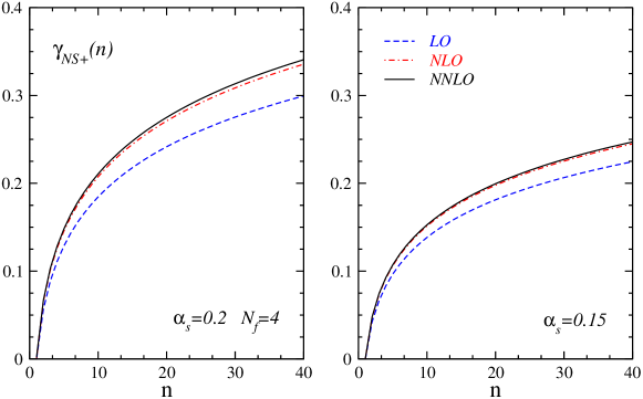
Figure 2: The perturbative expansion of the anomalous dimension $\gamma_{{}_{NS+}}(n)$ for four flavors at $\alpha_{s}=0.15,0.2$.

4 Parametrization of the parton densities

In this section we discuss how we can determine the valence quark densities at the input scale of $Q_{0}^{2}=1$ GeV². First of all, we should notice that the sum of the $u_{v}$ and $d_{v}$ distribution functions can be obtained from the CCFR data and not the two distributions separately. To separate the $xu_{v}$ and $xd_{v}$ contributions to $xF_{3}$ we need to use the relation between two distribution functions.

To start the parameterizations of the above mentioned parton distributions at the input scale of $Q_{0}^{2}$, we choose the following parametrization for the $u$-valence quark density

$$xu_{v}(x,Q_{0}^{2})=N_{u}x^{a}(1-x)^{b}(1+c\sqrt{x}+dx)\;.$$ (13)

In the above the $x^{a}$ term controls the low-$x$ behavior parton densities, and the $(1-x)^{b}$ terms the large $x$ values. The remaining polynomial factor accounts for additional medium-$x$ values. To separate the $xu_{v}$ and $xd_{v}$ contributions to $xF_{3}$ we assume the relation between two distribution functions as

$$\frac{d_{v}}{u_{v}}={\cal N}(1-x)^{e}\;,$$ (14)

this equation is same as the ratio which has reported in Ref.[40]. The parameter $e$ in this ratio is very important to control the behavior of $F_{3}$ for large $x$ value and the coefficient ${\cal N}$ is the normalization constant ($=\frac{N_{d}}{N_{u}}$). Therefor the parametrization of the $d$-valence quark density is as follows

$$xd_{v}(x,Q_{0}^{2})={\frac{N_{d}}{N_{u}}}(1-x)^{e}\;xu_{v}(x,Q_{0}^{2})\;.$$

Normalization constants $N_{u}$ and $N_{d}$ are fixed by

$$\int_{0}^{1}u_{v}(x)dx=C_{u}\;,$$ (15)

$$\int_{0}^{1}d_{v}(x)dx=C_{d}\;,$$ (16)

so normalization constants are equal to

$$N_{u}=\frac{C_{u}}{B(a,1+b)+cB(1/2+a,1+b)+dB(1+a,1+b)}\;,$$ (17)

$$N_{d}=\frac{C_{d}}{B(a,1+b+e)+cB(1/2+a,1+b+e)+dB(1+a,1+b+e)}\;,$$ (18)

here $C_{u}=2$ and $C_{d}=1$ are respectively the number of $u_{v}$ and $d_{v}$ quarks and $B(a,b)=\frac{\Gamma(a)\Gamma(b)}{\Gamma(a+b)}$ is the Euler Beta function.
The above normalizations are very effective to control unknown parameters in Eqs. (13,4) via the fitting procedure. The five parameters with $\Lambda_{QCD}^{N_{f}=4}$ will be extracted by using the Bernstain polynomials approach.

Using the valence quark distribution functions, the moments of $u_{v}(x,Q_{0}^{2})$ and $d_{v}(x,Q_{0}^{2})$ distributions can be easily calculated. The Mellin moments for the sum of the two valence quark distributions in the proton is as follows

$$u_{v}(N,Q_{0}^{2})+d_{v}(N,Q_{0}^{2}) = \int_{0}^{1}x^{N-2}\;\left(xu_{v}(x,Q_{0}^{2})+xd_{v}(x,Q_{0}^{2})\right)\;dx$$ (19)

$$= \int_{0}^{1}x^{N-2}\;xu_{v}(x,Q_{0}^{2})\left(1+\frac{N_{d}}{N_{u}}(1-x)^{e}\right)\;dx\;.$$

Now by inserting the above equation in the Eq. (12), the function of $f^{NS}(N,Q_{0}^{2})$ is determined in terms of unknown parameters $a,\;b,\;c,\;d,\;e$. This function is needed to determine the moments of non-singlet structure function in the related order.

5 Reconstruction of the structure function from moments

Although it is relatively easy to compute the $N$th moment from the structure functions, the inverse process is not obvious. To do this, we adopt a mathematically rigorous but easy method [41] to invert the moments and retrieve the structure functions. The method is based on the fact that for a given value of $Q^{2}$, only a limited number of experimental points, covering a partial range of values of $x$ are available. The method devised to deal with this situation is to take averages of the structure function weighted by suitable polynomials. We define the Bernstein polynomials as follows,

$$B_{nk}(x)=\frac{\Gamma(n+2)}{\Gamma(k+1)\Gamma(n-k+1)}x^{k}(1-x)^{n-k}\;;\;\;\;\;\;\;n\geq{k}.$$ (20)

These polynomials have a number of useful properties. These functions are normalized such that $\int_{0}^{1}B_{n,k}(x)dx=1$ and they are also constructed such that they are zero at endpoints $x=0$ and $x=1$. These polynomials are positive and have a single maximum located at

$$\bar{x}_{nk}(x) = \int_{0}^{1}x\;B_{nk}(x)\;dx$$ (21)

$$= \frac{\Gamma(n+2)\;\Gamma(k+2)}{\Gamma(n+3)\;\Gamma(k+1)}\;,$$

and finally, they are concentrated around this point, with a spread of

$$\Delta{x_{nk}} =\left[\int_{0}^{1}(x-\bar{x}_{nk})^{2}\;B_{nk}(x)\;dx\right]^{\frac{1}{2}}$$ (22)

$$=\sqrt{\frac{\Gamma(n+2)\;\Gamma(k+3)}{\Gamma(n+4)\;\Gamma(k+1)}-\left(\frac{{\Gamma(n+2)}\;{\Gamma(k+2)}}{{\Gamma(n+3)}\;{\Gamma(k+1)}}\right)^{2}}\;.$$

Therefore, for a given value of $Q^{2}$, the Bernstein averages of $F_{3}$ which are defined by,

$$F_{nk}(Q^{2}){\equiv}\int_{0}^{1}dxB_{nk}(x)F_{3}(x,Q^{2})\;,$$ (23)

represents an average of the function $F_{3}(x,Q^{2})$ in the region ${\bar{x}}_{nk}-\frac{1}{2}\Delta{x}_{nk}{\leq}x{\leq}{\bar{x}}_{nk}+\frac{1}{2}\Delta{x}_{nk}$. The key point is, the values of $F_{3}$ outside this interval have a small contribution to the above integral, as $B_{nk}(x)$ tends to zero very quickly. By a suitable choice of $n$, $k$ we manage to adjust to the region where the average is peaked around values which we have experimental data [28].

The construction of an acceptable average, and the resulting suppression of the missing data region is demonstrated in Fig. 3. In this figure the light grey region represents the interval ${\bar{x}}_{nk}-\frac{1}{2}\Delta{x}_{nk}{\leq}x{\leq}{\bar{x}}_{nk}+\frac{1}{2}\Delta{x}_{nk}$ and the dark grey areas represent the missing data regions. The small size of the dark grey region in the right hand plot demonstrates that this average has a negligible dependence on the missing data regions. Note that the right hand plot actually shows the integrand of the Bernstein average. The average itself will be this function integrated over $[0,1]$.

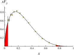
$$\;\times\;\frac{1}{x}\hskip 142.26378pt=\qquad$$

Figure 3: Constructing the Bernstein average, $F_{42}(Q^{2}=31.6)$. We see that the shaded (dark grey) missing data regions almost disappear in the right hand plot.

By expanding the integrand of Eq. (23) in powers of $x$, we can relate the averages directly to the moments,

$$F_{nk}(Q^{2})=\frac{{\Gamma(n+2)}}{\Gamma(k+1)}\sum_{l=0}^{n-k}\frac{(-1)^{l}}{l!(n-k-l)!}\int_{0}^{1}x^{(k+l+1)-1}{F_{3}(x,Q^{2})}dx\;,$$ (24)

and using the definition of Mellin moments of any hadron structure function, Eq. (4), we have

$$F_{nk}(Q^{2})=\frac{{\Gamma(n+2)}}{\Gamma(k+1)}\sum_{l=0}^{n-k}\frac{(-1)^{l}}{l!(n-k-l)!}\;{{\cal{M}}({(k+l)+1}},Q^{2})\;.$$ (25)

We can only include a Bernstein average, $F_{nk}$, if we have experimental points covering the whole range [${\bar{x}}_{nk}-\frac{1}{2}\Delta{x}_{nk},{\bar{x}}_{nk}+\frac{1}{2}\Delta{x}_{nk}$] [42],[43],[44]. This means that with the available experimental data we can only use the following 28 averages, including $F_{21}^{(exp)}(Q^{2})$, $F_{31}^{(exp)}(Q^{2})$, $F_{42}^{(exp)}(Q^{2})$, … . Using Eq. (25), the 28 Bernstein averages ${F}_{nk}({Q}^{2})$ can be written in terms of odd and even moments. For instance:

$${F_{21}}(Q^{2})=6\left({\cal{M}}(2,Q^{2})-{\cal{M}}(3,Q^{2})\right)\;,$$

$${F_{31}}(Q^{2})=24\left(0.5\;{\cal{M}}(2,Q^{2})-{\cal{M}}(3,Q^{2})+0.5\;{\cal{M}}(4,Q^{2})\right)\;,$$

$${F_{42}}(Q^{2})=60\left(0.5\;{\cal{M}}(3,Q^{2})-{\cal{M}}(4,Q^{2})+0.5\;{\cal{M}}(5,Q^{2})\right)\;,$$

$$\vdots$$ (26)

We can now compare the theoretical predictions with the experimental results for the Bernstein averages. Another restriction we assume here, is to ignore the effects of moments with high order $n$ which do not strongly constrain the fits. To obtain these experimental averages from CCFR data [28], we fit $x{F_{3}}(x,{Q^{2}})$ for each bin in ${Q}^{2}$ separately to the phenomenologically convenient expression given in Eq. (1). Using Eq. (1) with the fitted values of ${\cal{A}},{\cal{B}}$ and ${\cal{C}}$, one can then compute ${F}_{nk}^{(exp)}({Q}^{2})$ using Eq. (24), in terms of Gamma functions. Some sample experimental Bernstein averages are plotted in Fig. 4 in the higher approximations. The errors in the ${F}_{nk}^{(exp)}(Q^{2})$ correspond to allowing the CCFR data for $x{F}_{3}$ to vary within the experimental error bars, including the experimental systematic and statistical errors [28].
The unknown parameters according to Eqs. (13,4) will be $a,b,c,d,e$ and $\Lambda_{QCD}^{N_{f}}$. Thus, there are 6 parameters for each order to be simultaneously fitted to the experimental ${F}_{nk}({Q}^{2})$ averages. Using the CERN subroutine MINUIT [45], we defined a global ${\chi}^{2}$ for all the experimental data points and found an acceptable fit with minimum ${\chi}^{2}/{\rm{dof}}=92.259/134=0.688$ in the LO case, $77.452/134=0.578$ in the NLO and $74.772/134=0.558$ in the NNLO case. The best fit is indicated by some sample curves in Fig. 4. The fitting parameters with their uncertainties and the minimum ${\chi}^{2}$ values in each order are listed in Table 2.

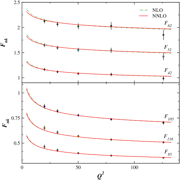
Figure 4: NLO and NNLO fits to Bernstein averages of $xF_{3}$.

From Eqs.(13,4), we are now able to determine the $xu_{v}$ and $xd_{v}$ at the scale of $Q_{0}^{2}$ in higher order corrections. In Fig. 5 we have plotted the NLO and NNLO approximation results of $xu_{v}$ and $xd_{v}$ with correlated errors at the input scale $Q_{0}^{2}=1.0$ GeV² (solid line) compared to results obtained from NNLO analysis (left panels) and NLO analysis (right panels) by BBG [46] (dashed line), MRST (dashed-dotted line) [47] and A05(dashed-dotted-dotted line) [48].

		LO	NLO	NNLO
$u_{v}$	$N_{u}$	$1.952$	$3.942$	$5.134$
	$a$	$0.570\pm 0.016$	$0.777\pm 0.020$	$0.830\pm 0.019$
	$b$	$3.300\pm 0.089$	$3.548\pm 0.032$	$3.724\pm 0.039$
	$c$	$-0.380\pm 0.040$	$0.410\pm 0.039$	$0.040\pm 0.004$
	$d$	$4.900\pm 0.136$	$1.500\pm 0.027$	$1.449\pm 0.104$
$d_{v}$	$N_{d}$	$1.308$	$2.620$	$3.348$
	$e$	$1.699\pm 0.135$	$1.563\pm 0.014$	$1.460\pm 0.020$
$\Lambda_{QCD}^{N_{f}=4},MeV$		$211\pm 27$	$259\pm 18$	$230\pm 12$
$\chi^{2}/ndf$		$92.259/134=0.688$	$77.452/134=0.578$	$74.772/134=0.558$

Table 2: Parameter values of the LO, NLO, and NNLO non-singlet QCD fit at $Q_{0}^{2}=1$ GeV².

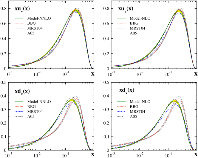
Figure 5: The parton densities $xu_{v}$ and $xd_{v}$ at the input scale $Q_{0}^{2}=1.0$ GeV² (solid line) compared to results obtained from NNLO analysis (left panels) and NLO analysis (right panels) by BBG [46] (dashed line), MRST (dashed-dotted line) [47] and A05 (dashed-dotted-dotted line) [48].

All of the non-singlet parton distribution functions in moment space for any order are now available, so we can use the inverse Mellin technic to obtain the $Q^{2}$ evolution of valance quark distributions which will be done in the next section.

6 Valence quark densities in the $\bf{x}$-space

In the previous section we parameterized the non-singlet parton distribution functions at input scale of $Q_{0}^{2}=1$ GeV² in the LO, NLO and NNLO approximations by using Bernstein averages method. To obtain the non-singlet parton distribution functions in $x$-space and for $Q^{2}>Q_{0}^{2}$ GeV² we need to use the non-singlet evolution equation for parton densties to 3-loop order in Eq.(10). To obtain the $x$-dependence of parton distributions from the $N-$dependent exact analytical solutions in the Mellin-moment space, one has to perform a numerical integral in order to invert the Mellin-transformation [49]

$$q_{v}(x,Q^{2})=\frac{1}{\pi}\int_{0}^{\infty}dwIm[e^{i\phi}x^{-c-we^{i\phi}}M_{q_{v}}(N=c+we^{i\phi},Q^{2})]\;,$$ (27)

with $q_{v}=u_{v},d_{v}$. In this equation the contour of the integration lies on the right of all singularities of $M_{q_{v}}(N=c+we^{i\phi},Q^{2})$ in the complex $N$-plane. For all practical purposes one may choose $c\simeq 1,\phi=135^{\circ}$ and an upper limit of integration, for any $Q^{2}$, of about $5+10/\ln x^{-1}$, instead of infinity, which guarantees stable numerical results [50, 51]. In this way, we can obtain all valence distribution functions in fixed $Q^{2}$ and in $x$-space. In Fig. 6 we have presented the parton distribution $xu_{v}$ at some different values of $Q^{2}$. These distributions were compared to LO , NLO and NNLO approximations with some theoretical models [47, 48, 52].
In Fig. 7 we have presented the same distributions for $xd_{v}$. We should notice that in Figs. 5,  6 and  7 the minimum value of $Q^{2}$ from [47] and [52] is $1.25$ GeV² and $1.3$ GeV² respectively.
In Table 4 comparison of low order moments at $Q^{2}=4$ GeV² from our non-singlet NNLO QCD analysis with the NNLO analysis BBG06 [46], MRST04 [47], A02 [48] and A06 [53] has been done.

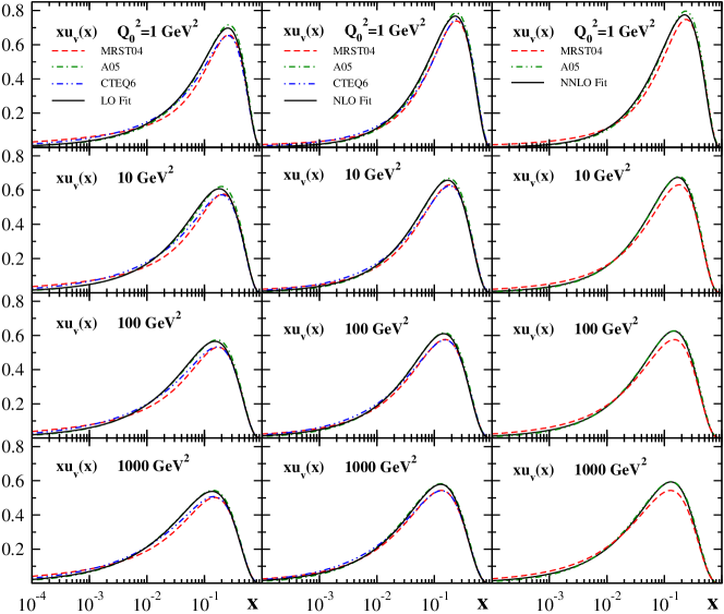
Figure 6: The parton distribution $xu_{v}$ at some different values of $Q^{2}$. The solid line is our model, dashed line is the MRST model [47], dashed-dotted line is the A05 model [48] and dashed-dotted-dotted line is the CTEQ model [52].

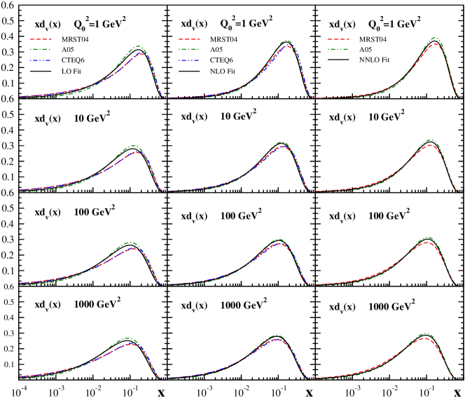
Figure 7: The parton distribution $xd_{v}$ at some different values of $Q^{2}$. The solid line is our model, dashed line is the MRST model [47], dashed-dotted line is the A05 model [48] and dashed-dotted-dotted line is the CTEQ model [52].

$f$	$N$	NNLO	BBG06	MRST04	A02	A06
$u_{v}$	2	0.2934 $\pm$ 0.0036	0.2986 $\pm$ 0.0029	0.285	0.304	0.2947
	3	0.0825 $\pm$ 0.0012	0.0871 $\pm$ 0.0011	0.082	0.087	0.0843
	4	0.0311 $\pm$ 0.0004	0.0333 $\pm$ 0.0005	0.032	0.033	0.0319
$d_{v}$	2	0.1143 $\pm$ 0.0013	0.1239 $\pm$ 0.0026	0.115	0.120	0.1129
	3	0.0262 $\pm$ 0.0003	0.0315 $\pm$ 0.0008	0.028	0.028	0.0275
	4	0.0083 $\pm$ 0.0001	0.0105 $\pm$ 0.0004	0.009	0.010	0.0092

Table 4: Comparison of low order moments at $Q^{2}=4$ GeV² from our non-singlet NNLO QCD analysis with the NNLO analysis BBG06 [46], MRST04 [47], A02 [48] and A06 [53].

7 Conclusion

The QCD analysis is performed in LO, NLO and NNLO based on Bernstein polynomial approach. We determine the valence quark densities in a wide range of $x$ and $Q^{2}$. The QCD scale $\Lambda_{\rm QCD}^{\rm N_{f}=4}$ is determined together with the parameters of the parton distributions. In Table 5 we have summarized our fit results comparing $\Lambda_{\rm QCD}^{\rm N_{f}=4}$ and $\alpha_{s}(M_{Z}^{2})$ for the LO, NLO and NNLO analysis. The LO value of $\Lambda_{\rm QCD}^{\rm N_{f}=4}$ is found to be smaller than the NLO value, while the NLO value comes out somewhat higher than the NNLO value.

	$\Lambda_{QCD}^{N_{f}=4}$, MeV	$\alpha_{s}(M_{Z}^{2})$
LO	$211\pm 27$	$0.1291\pm 0.0025$
NLO	$259\pm 18$	$0.1150\pm 0.0011$
NNLO	$230\pm 12$	$0.1142\pm 0.0008$

Table 5: $\Lambda_{\mathrm{QCD}}^{\mathrm{N_{f}=4}}$ and $\alpha_{s}(M_{Z}^{2})$ at LO, NLO and NNLO.

We compare the results of the present analysis to results [34], [46], [48], [52-57] obtained in the literature at NLO and NNLO in Table 6, where most of the NLO values for $\alpha_{s}(M_{Z}^{2})$ presented are determined in combined singlet- and non-singlet analysis. The NLO values for $\alpha_{s}(M_{Z}^{2})$ are larger than those at NNLO in several analysis. The difference of both values, however, is not always the same. This is most likely due to the type of the analysis being performed (singlet and non-singlet, non-singlet only, etc.), in which also partly different data sets are analyzed. Non-singlet QCD analysis were also performed for neutrino data by using Jacobi polynomial method. In [33] the CCFR iron data on $xF_{3}(x,Q^{2})$ [28] were analyzed in NLO and NNLO using fixed moments. Likewise a NNLO analysis was performed in [34]. In [33] rather large values for $\Lambda_{\rm QCD}^{\rm N_{f}=4,\overline{\rm MS}}$: $\Lambda_{\rm QCD,NLO}^{\rm N_{f}=4,\overline{\rm MS}}=371\pm 72\,\mbox{MeV}$, $\Lambda_{\rm QCD,NNLO}^{\rm N_{f}=4,\overline{\rm MS}}=316\pm 51\,\mbox{MeV}$ are obtained, which are larger than the values obtained in the analysis based on $F_{2}^{p,d}(x,Q^{2})$ data, still showing the pattern that the NNLO value is lower than the NLO value. In Ref.  [34] one finds $\Lambda_{\rm QCD,NLO}^{\rm N_{f}=4,\overline{\rm MS}}=281\pm 57\,\mbox{MeV}$, $\Lambda_{\rm QCD,NNLO}^{\rm N_{f}=4,\overline{\rm MS}}=255\pm 55\,\mbox{MeV}$.

And finally in [46] with the QCD analysis of deep inelastic world data, the value of $\Lambda_{\rm QCD}^{\rm N_{f}=4,\overline{\rm MS}}$ is reported as

$$\Lambda_{\rm QCD,NLO}^{\rm N_{f}=4,\overline{\rm MS}} = 265\pm 27\,\mbox{MeV}$$ (28)

$$\Lambda_{\rm QCD,NNLO}^{\rm N_{f}=4,\overline{\rm MS}} = 226\pm 25\,\mbox{MeV}~{}.$$ (29)

which seems close to results of the present analysis. We believe that the difference of the reported value above, not only depends on the type of analysis being performed (singlet and non-singlet, non-singlet only, etc.) but also on the kind of approach ($N$-space, x-space, etc.) have been taken.

	$\alpha_{s}(M_{Z}^{2})$	Ref.
NLO
CTEQ6	$0.1165\pm 0.0065$	[52]
MRST03	$0.1165\pm 0.0020$	[54]
A02	$0.1171\pm 0.0015$	[48]
ZEUS	$0.1166\pm 0.0049$	[55]
H1	$0.1150\pm 0.0017$	[56]
GRS	$0.112$	[57]
BBG	$0.1148\pm 0.0019$	[46]
Model	$0.1150\pm 0.0011$
NNLO
MRST03	$0.1153\pm 0.0020$	[54]
A02	$0.1143\pm 0.0014$	[48]
SY01(ep)	$0.1166\pm 0.0013$	[34]
SY01($\nu$N)	$0.1153\pm 0.0063$	[34]
GRS	$0.111$	[57]
A06	$0.1128\pm 0.0015$	[53]
BBG	$0.1134^{+0.0019}_{-0.0021}$	[46]
Model	$0.1142\pm 0.0008$

Table 6: Comparison of $\alpha_{s}(M_{Z}^{2})$ values from NLO, and NNLO QCD analysis.

Another important characteristic of the deep inelastic neutrino-nucleon scattering is the Gross-Llewellyn Smith (GLS) sum rule [58]

$$GLS(Q^{2})=\frac{1}{2}\int_{0}^{1}\frac{xF_{3}^{\bar{\nu}p+\nu p}(x,Q^{2})}{x}dx\;.$$ (30)

In the work of Ref. [59], the following result of the measurement of the GLS sum at the scale $\mid Q^{2}\mid=3$ GeV² was reported:

$$GLS(\mid Q^{2}\mid=3\;GeV^{2})=2.5\pm 0.018(stat.)\pm 0.078(syst.)$$ (31)

In Ref. [60] the GLS($\mid Q_{0}^{2}\mid=3$ GeV²) were analyzed based on the Jacobi polynomials expansion method. The value of GLS in the NLO approximation is reported as GLS(3 GeV²)=2.446$\pm 0.081$ [60], which is in agreement with the results Eq. (31). We should notice that in order to obtain NLO expression for the GLS sum rule one should consider the NNLO approximation of the moments ${\cal M}(N,Q^{2})$. Following Ref. [60], we analyze the GLS sum rule with the corresponding perturbative QCD predictions for the first Mellin moments, and obtain

$$GLS(\mid Q^{2}\mid=3\;GeV^{2})=2.40\pm 0.06$$ (32)

We hope to report on the application of the methods employed in the present work to describe more complicated hadron structure functions, and on using the singlet case to extract parton densities in three loop in future works.

8 Acknowledgments

We are especially grateful to G. Altarelli for fruitful suggestions, discussions and critical remarks. We wish to thank J. Blümlein for giving us his useful and constructive comments about flavor threshold matching. A.N.K is thanking to F. James and I. Maclaren for discussion about MINUIT CERN program library. We would like to thank M. M. Sheikh Jabbari, M. Ghominejad for reading the manuscript of this paper and for useful discussions. A. Mirjalili is thanked for useful discussions. A.N.K is grateful to CERN for their hospitality whilst he visited there and could amend this paper. We acknowledge the Institute for Studies in Theoretical Physics and Mathematics (IPM) and Semnan university for the financial support of this project.

References

- [1] D. J. Gross and F. Wilczek, “Asymptotically Free Gauge Theories. 1,” Phys. Rev. D 8 (1973) 3633.
- [2] H. Georgi and H. D. Politzer, “Electroproduction scaling in an asymptotically free theory of strong interactions,” Phys. Rev. D 9 (1974) 416.
- [3] G. Altarelli and G. Parisi, “Asymptotic Freedom In Parton Language,” Nucl. Phys. B 126 (1977) 298.
- [4] E. G. Floratos, D. A. Ross and C. T. Sachrajda, “Higher Order Effects In Asymptotically Free Gauge Theories: The Anomalous Dimensions Of Wilson Operators,” Nucl. Phys. B 129 (1977) 66 [Erratum-ibid. B 139 (1978) 545].
- [5] E. G. Floratos, D. A. Ross and C. T. Sachrajda, “Higher Order Effects In Asymptotically Free Gauge Theories. 2. Flavor Singlet Wilson Operators And Coefficient Functions”, Nucl. Phys. B 152 (1979) 493.
- [6] A. Gonzalez-Arroyo, C. Lopez and F. J. Yndurain, “Second Order Contributions To The Structure Functions In Deep Inelastic Scattering. I. Theoretical Calculations,” Nucl. Phys. B 153 (1979) 161.
- [7] A. Gonzalez-Arroyo and C. Lopez, “Second Order Contributions To The Structure Functions In Deep Inelastic Scattering. 3. The Singlet Case,” Nucl. Phys. B 166 (1980) 429.
- [8] G. Curci, W. Furmanski and R. Petronzio, “Evolution Of Parton Densities Beyond Leading Order: The Nonsinglet Case,” Nucl. Phys. B 175 (1980) 27.
- [9] W. Furmanski and R. Petronzio, “Singlet Parton Densities Beyond Leading Order,” Phys. Lett. B 97 (1980) 437.
- [10] E. G. Floratos, C. Kounnas and R. Lacaze, “Higher Order QCD Effects In Inclusive Annihilation And Deep Inelastic Scattering,” Nucl. Phys. B 192 (1981) 417.
- [11] R. Hamberg and W. L. van Neerven, “The Correct renormalization of the gluon operator in a covariant gauge,” Nucl. Phys. B 379 (1992) 143.
- [12] W. L. van Neerven and E. B. Zijlstra, “Order Alpha-S**2 Contributions To The Deep Inelastic Wilson Coefficient,” Phys. Lett. B 272 (1991) 127.
- [13] E. B. Zijlstra and W. L. van Neerven, “Contribution Of The Second Order Gluonic Wilson Coefficient To The Deep Inelastic Structure Function,” Phys. Lett. B 273 (1991) 476.
- [14] E. B. Zijlstra and W. L. van Neerven, “Order Alpha-S**2 correction to the structure function in deep inelastic neutrino - hadron scattering,” Phys. Lett. B 297 (1992) 377.
- [15] E. B. Zijlstra and W. L. van Neerven, “Order Alpha-S**2 QCD Corrections To The Deep Inelastic Proton Structure Functions F2 And F(L),” Nucl. Phys. B 383 (1992) 525.
- [16] R. Hamberg, W. L. van Neerven and T. Matsuura, “A Complete calculation of the order alpha-s**2 correction to the Drell-Yan K factor,” Nucl. Phys. B 359 (1991) 343 [Erratum-ibid. B 644 (2002) 403].
- [17] R. V. Harlander and W. B. Kilgore, “Next-to-next-to-leading order Higgs production at hadron colliders,” Phys. Rev. Lett. 88 (2002) 201801 [arXiv:hep-ph/0201206].
- [18] C. Anastasiou, L. J. Dixon, K. Melnikov and F. Petriello, “Dilepton rapidity distribution in the Drell-Yan process at NNLO in QCD,” Phys. Rev. Lett. 91 (2003) 182002 [arXiv:hep-ph/0306192].
- [19] C. Anastasiou, L. J. Dixon, K. Melnikov and F. Petriello, “High-precision QCD at hadron colliders: Electroweak gauge boson rapidity distributions at NNLO,” Phys. Rev. D 69 (2004) 094008 [arXiv:hep-ph/0312266].
- [20] C. Anastasiou and K. Melnikov, “Higgs boson production at hadron colliders in NNLO QCD,” Nucl. Phys. B 646 (2002) 220 [arXiv:hep-ph/0207004].
- [21] V. Ravindran, J. Smith and W. L. van Neerven, “NNLO corrections to the total cross section for Higgs boson production in hadron hadron collisions,” Nucl. Phys. B 665 (2003) 325 [arXiv:hep-ph/0302135].
- [22] R. V. Harlander and W. B. Kilgore, “Higgs boson production in bottom quark fusion at next-to-next-to-leading order,” Phys. Rev. D 68 (2003) 013001 [arXiv:hep-ph/0304035].
- [23] E. W. N. Glover, “Progress in NNLO calculations for scattering processes,” Nucl. Phys. Proc. Suppl. 116 (2003) 3 [arXiv:hep-ph/0211412].
- [24] S. A. Larin, T. van Ritbergen and J. A. M. Vermaseren, “The Next Next-To-Leading QCD Approximation For Nonsinglet Moments Of Deep Inelastic Structure Functions,” Nucl. Phys. B 427 (1994) 41.
- [25] S. A. Larin, P. Nogueira, T. van Ritbergen and J. A. M. Vermaseren, “The 3-loop QCD calculation of the moments of deep inelastic structure functions,” Nucl. Phys. B 492 (1997) 338 [arXiv:hep-ph/9605317].
- [26] A. Retey and J. A. M. Vermaseren, “Some higher moments of deep inelastic structure functions at next-to-next-to leading order of perturbative QCD,” Nucl. Phys. B 604 (2001) 281 [arXiv:hep-ph/0007294].
- [27] S. Moch, J. A. M. Vermaseren and A. Vogt, “The three-loop splitting functions in QCD: The non-singlet case,” Nucl. Phys. B 688 (2004) 101 [arXiv:hep-ph/0403192].
- [28] W. G. Seligman et al., “Improved determination of alpha(s) from neutrino nucleon scattering,” Phys. Rev. Lett. 79, (1997) 1213.
- [29] A. L. Kataev, A. V. Kotikov, G. Parente and A. V. Sidorov, “Next-to-next-to-leading order QCD analysis of the revised CCFR data for xF3 structure function,” Phys. Lett. B 417, (1998) 374 [arXiv:hep-ph/9706534].
- [30] A. L. Kataev, G. Parente and A. V. Sidorov, “The QCD analysis of the CCFR data for xF3: Higher twists and alpha(s)(M(Z)) extractions at the NNLO and beyond,” arXiv:hep-ph/9809500.
- [31] S. I. Alekhin and A. L. Kataev, “The NLO DGLAP extraction of alpha(s) and higher twist terms from CCFR xF3 and F2 structure functions data for nu N DIS,” Phys. Lett. B 452, (1999) 402 [arXiv:hep-ph/9812348].
- [32] A. L. Kataev, G. Parente and A. V. Sidorov, “Higher twists and alpha(s)(M(Z)) extractions from the NNLO QCD analysis of the CCFR data for the xF3 structure function,” Nucl. Phys. B 573, (2000) 405 [arXiv:hep-ph/9905310].
- [33] A. L. Kataev, G. Parente and A. V. Sidorov, “Fixation of theoretical ambiguities in the improved fits to the xF3 CCFR data at the next-to-next-to-leading order and beyond,” Phys. Part. Nucl. 34, (2003) 20 [arXiv:hep-ph/0106221]; A. L. Kataev, G. Parente and A. V. Sidorov, “N3LO fits to xF3 data: alpha(s) vs 1/Q**2 contributions,” Nucl. Phys. Proc. Suppl. 116 (2003) 105 [arXiv:hep-ph/0211151].
- [34] J. Santiago and F. J. Yndurain, “Improved calculation of F2 in electroproduction and xF3 in neutrino scattering to NNLO and determination of alpha(s),” Nucl. Phys. B 611, (2001) 447 [arXiv:hep-ph/0102247].
- [35] A. Vogt, “Efficient evolution of unpolarized and polarized parton distributions with QCD-PEGASUS,” Comput. Phys. Commun. 170, (2005) 65 [arXiv:hep-ph/0408244].
- [36] K. G. Chetyrkin, B. A. Kniehl and M. Steinhauser, “Strong coupling constant with flavour thresholds at four loops in the MS-bar scheme,” Phys. Rev. Lett. 79 (1997) 2184 [arXiv:hep-ph/9706430].
- [37] S. Bethke, “Determination of the QCD coupling alpha(s),” J. Phys. G 26 (2000) R27 [arXiv:hep-ex/0004021].
- [38] W. A. Bardeen, A. J. Buras, D. W. Duke and T. Muta, “Deep Inelastic Scattering Beyond The Leading Order In Asymptotically Free Gauge Theories,” Phys. Rev. D 18 (1978) 3998.
- [39] S. Moch and J. A. M. Vermaseren, “Deep inelastic structure functions at two loops,” Nucl. Phys. B 573, (2000) 853 [arXiv:hep-ph/9912355].
- [40] M. Diemoz, F. Ferroni, E. Longo and G. Martinelli, “PARTON DENSITIES FROM DEEP INELASTIC SCATTERING TO HADRONIC PROCESSES AT SUPER COLLIDER ENERGIES,” Z. Phys. C 39 (1988) 21; M. Gluck, E. Reya and A. Vogt, “Radiatively Generated Parton Distributions For High-Energy Collisions,” Z. Phys. C 48 (1990) 471; M. Gluck, E. Reya and A. Vogt, “Dynamical parton distributions revisited,” Eur. Phys. J. C 5 (1998) 461 [arXiv:hep-ph/9806404].
- [41] F. J. Yndurain, “Reconstruction Of The Deep Inelastic Structure Functions From Their Moments,” Phys. Lett. B 74 (1978) 68.
- [42] C. J. Maxwell and A. Mirjalili, “Direct extraction of QCD Lambda(MS-bar) from moments of structure functions in neutrino nucleon scattering, using the CORGI approach,” Nucl. Phys. B 645 (2002) 298 [arXiv:hep-ph/0207069]; P. M. Brooks and C. J. Maxwell, “Improved analysis of moments of F3 in neutrino nucleon scattering using the Bernstein polynomial method,” [arXiv:hep-ph/0610137].
- [43] A. N. Khorramian, A. Mirjalili and S. A. Tehrani, “Next-to-leading order approximation of polarized valon and parton distributions,” JHEP 0410 (2004) 062 [arXiv:hep-ph/0411390].
- [44] J. Santiago and F. J. Yndurain, “Calculation of electroproduction to NNLO and precision determination of alpha(s),” Nucl. Phys. B 563 (1999) 45 [arXiv:hep-ph/9904344]; J. Santiago and F. J. Yndurain, “Improved calculation of F2 in electroproduction and xF3 in neutrino scattering to NNLO and determination of alpha(s),” Nucl. Phys. B 611 (2001) 447 [arXiv:hep-ph/0102247].
- [45] F. James, CERN Program Library Long Writeup D506, (1994).
- [46] J. Blumlein, H. Bottcher and A. Guffanti, “Non-singlet QCD analysis of deep inelastic world data at O(alpha(s)3),” arXiv:hep-ph/0607200; J. Blumlein, H. Bottcher and A. Guffanti, “NNLO analysis of unpolarized DIS structure functions,” arXiv:hep-ph/0606309.
- [47] A. D. Martin, R. G. Roberts, W. J. Stirling and R. S. Thorne, “Physical gluons and high-E(T) jets,” Phys. Lett. B 604, (2004) 61 [arXiv:hep-ph/0410230].
- [48] S. Alekhin, “Parton distribution functions from the precise NNLO QCD fit,” JETP Lett. 82, 628 (2005) [Pisma Zh. Eksp. Teor. Fiz. 82, 710 (2005)] [arXiv:hep-ph/0508248]; S. Alekhin, “Parton distributions from deep-inelastic scattering data,” Phys. Rev. D 68 (2003) 014002 [arXiv:hep-ph/0211096].
- [49] D. Graudenz, M. Hampel, A. Vogt and C. Berger, “The Mellin transform technique for the extraction of the gluon density,” Z. Phys. C 70, (1996) 77 [arXiv:hep-ph/9506333].
- [50] M. Gluck, E. Reya and A. Vogt, “Radiatively Generated Parton Distributions For High-Energy Collisions,” Z. Phys. C 48 (1990) 471.
- [51] M. Gluck, E. Reya and A. Vogt, “Parton Structure Of The Photon Beyond The Leading Order,” Phys. Rev. D 45 (1992) 3986.
- [52] J. Pumplin, D. R. Stump, J. Huston, H. L. Lai, P. Nadolsky and W. K. Tung, “New generation of parton distributions with uncertainties from global QCD analysis,” JHEP 0207 (2002) 012 [arXiv:hep-ph/0201195].
- [53] S. Alekhin, K. Melnikov and F. Petriello, “Fixed target Drell-Yan data and NNLO QCD fits of parton distribution functions,” arXiv:hep-ph/0606237.
- [54] A. D. Martin, R. G. Roberts, W. J. Stirling and R. S. Thorne, “MRST partons and uncertainties,” arXiv:hep-ph/0307262.
- [55] S. Chekanov et al. [ZEUS Collaboration], “A ZEUS next-to-leading-order QCD analysis of data on deep inelastic scattering,” Phys. Rev. D 67 (2003) 012007 [arXiv:hep-ex/0208023].
-
[56]
C. Adloff et al. [H1 Collaboration], “Deep-inelastic
inclusive e p scattering at low x and a determination of alpha(s),”
Eur. Phys. J. C 21 (2001) 33
[arXiv:hep-ex/0012053];
- [57] M. Glück, E. Reya and C. Schuck, “Non-singlet QCD analysis of F2(x,Q2) up to NNLO,” arXiv:hep-ph/0604116.
- [58] D. J. Gross and C. H. Llewellyn Smith, “High-energy neutrino - nucleon scattering, current algebra and partons,” Nucl. Phys. B 14 (1969) 337.
- [59] W. C. Leung et al., “A Measurement Of The Gross-Llewellyn-Smith Sum Rule From The CCFR Structure Function,” Phys. Lett. B 317 (1993) 655.
- [60] A. L. Kataev and A. V. Sidorov, “The Jacobi Polynomials QCD Analysis Of The CCFR Data For And The Q2 Dependence Of The Gross-Llewellyn-Smith Sum Rule,” Phys. Lett. B 331 (1994) 179 [arXiv:hep-ph/9402342].