CP violation and electric-dipole-moment at low energy $\tau$ production with polarized electrons

Abstract

The new proposals for high luminosity B/Flavor factories, near and on top of the $\Upsilon$ resonances, allow for a detailed investigation of $CP$-violation in the $\tau$-pair production. In particular, bounds on the tau electric dipole moment can be obtained from genuine CP-odd observables related to the $\tau$-pair production. We perform an independent analysis from low energy (10 GeV) data by means of linear spin observables. We show that for a longitudinally polarized electron beam a $CP$-odd asymmetry, associated to the normal polarization term, can be measured at these low energy facilities both at resonant and non resonant energies. In this way stringent and independent bounds to the tau electric dipole moment, which are orders of magnitude below other high or low energy bounds, can be obtained.

, and

1 Introduction

The standard model describes with high accuracy most of the physics found in present experiments [1]. Nowadays, however, neutrino physics offers a first clue to physics beyond this ”low energy” model [2]. Other signals of new phenomena may also appear in CP violation physics. While CP violation in the standard model can be easily introduced by quark mixing, as in the CKM mechanism, the discovery of CP violation in the lepton sector would establish new sources of CP violation and the appearance of new physics. The time reversal odd electric dipole moment (EDM) of the $\tau$ is the source of CP violation in the $\tau$-pair production vertex. In the framework of local quantum field theories the CPT theorem states that CP violation is equivalent to T violation. While the T-odd electric dipole moments (EDM) of the electron and muon have been extensively investigated both in experiment and theory, the case of the tau is somewhat different. The dipole moment effective operators flip chirality and are therefore related to the mass mechanism of the theory. The tau lepton has a relatively high mass: this means that tau lepton physics is expected to be more sensitive to contributions to chirality-flip terms coming from high energy scales and new physics. Furthermore, the tau has a very short lifetime and can decay into hadrons, so different techniques to those for the (stable) electron or muon case are needed in order to measure the dipole moments. There are very precise bounds on the EDM magnitude of nucleons and leptons; the most precise one is the electron EDM, $d^{e}_{\gamma}=(0.07\pm 0.07)\times 10^{-26}$ e cm, while the looser one is the $\tau$ EDM [1], $-0.22\,\it{e\,cm}<Re(d^{\tau}_{\gamma})\times 10^{16}<0.45\,\it{e\,cm}$. From the theoretical point of view the CP violation mechanisms in many models provide a kind of accidental protection in order to generate an EDM for quarks and leptons. This is the case in the CKM mechanism, where EDM and weak-EDM are generated only at very high order in the coupling constant. This opens a way to test many models: $CP$-odd observables related to EDM would give no appreciable effect from the standard model and any experimental signal should be identified with beyond the standard model physics. Following the ideas of [3] and [4], the tau weak-EDM has been studied in $CP$-odd observables [5, 6] at high energies through linear polarizations and spin-spin correlations. EDM bounds for the tau, from $CP$-even observables such as total cross sections or decay widths, have also been considered in [7, 8, 9]. In ref.[10] the sensitivity to the WEDM in spin-spin correlation observables was studied for tau-charm-factories with polarized electrons. While most of the statistics for the tau pair production was dominated in the past by high energy physics, mainly at LEP, nowadays the situation has evolved. High luminosity B factories and their upgrades at resonant energies ($\Upsilon$ thresholds) have the largest $\tau$ pair samples. In the future, the possibility for a Super B/Flavor Factory with a $\tau$-pair production rates many orders of magnitude higher than present samples is being intensively analyzed [11]. These facilities may also have the possibility of polarized beams. This calls for a dedicated study of the observables related to CP violation and the EDM of the $\tau$ lepton at low energies. In this paper we study a set of different observables for the tau system that may lead to competitive results with the present bounds for the EDM.

2 Effective Lagrangian

Deviations from the standard model, at low energies, can be parametrized by an effective Lagrangian built with the standard model particle spectrum, having as zero order term just the standard model Lagrangian, and containing higher dimension gauge invariant operators suppressed by the scale of new physics, $\Lambda$ [12]. The leading non-standard effects come from the operators with the lowest dimension. For CP violation those are dimension six operators and there are only two operators of this type that contribute [13] to the tau EDM and weak-EDM:

$$\mathcal{O}_{B}=\frac{g^{\prime}}{2\Lambda^{2}}\overline{L_{L}}\varphi\sigma_{\mu\nu}\tau_{R}B^{\mu\nu}~{}, \hskip 28.45274pt\mathcal{O}_{W}=\frac{g}{2\Lambda^{2}}\overline{L_{L}}\vec{\tau}\varphi\sigma_{\mu\nu}\tau_{R}\vec{W}^{\mu\nu}~{}.$$ (1)

Here $L_{L}=(\nu_{L},\tau_{L})$ is the tau leptonic doublet, $\varphi$ is the Higgs doublet, $B^{\nu\nu}$ and $\vec{W}^{\mu\nu}$ are the U(1)_Y and SU(2)_L field strength tensors, and $g^{\prime}$ and $g$ are the gauge couplings.

Other possible operators that one could imagine reduce to the above ones of Eq.(1) after using the standard model equations of motion. In so doing, the couplings will be proportional to the tau-lepton Yukawa couplings.

Thus, the effective Lagrangian for the EDM is:

$$\mathcal{L}_{eff}=i\alpha_{B}\mathcal{O}_{B}+i\alpha_{W}\mathcal{O}_{W}+\mathrm{h.c.}$$ (2)

where the couplings $\alpha_{B}$ and $\alpha_{W}$ are real. Note that complex couplings do not break $CP$ conservation and lead to magnetic dipole moments which are not considered in this paper where we are mainly interested on $CP$-odd observables.

After spontaneous symmetry breaking the neutral scalar gets a vacuum expectation value and the interactions in Eq.(2) can be written in terms of the gauge boson mass eigenstates $A^{\mu}$ and $Z^{\mu}$ as:

$$\mathcal{L}_{eff}^{\gamma,Z} = -i\,d^{\tau}_{\gamma}\,\overline{\tau}\sigma_{\mu\nu}\gamma^{5}\tau F^{\mu\nu}-i\,d^{\tau}_{Z}\,\overline{\tau}\sigma_{\mu\nu}\gamma^{5}\tau Z^{\mu\nu}$$ (3)

where $F_{\mu\nu}=\partial_{\mu}A_{\nu}-\partial_{\nu}A_{\mu}$ and $Z_{\mu\nu}=\partial_{\mu}Z_{\nu}-\partial_{\nu}Z_{\mu}$ are the abelian field strength tensors of the photon and $Z$ gauge boson and $d^{\tau}_{\gamma}$ and $\d^{\tau}_{Z}$ are the electric and weak-electric dipole moments, respectively. We have not written in Eq.(3) some of the terms coming from Eq.(2) because they do not contribute at leading order to the observables we are interested in. These terms are the non-abelian couplings involving more than one gauge boson and the term related to the $CP$-odd $\nu_{\tau}-\tau-W^{\pm}$ couplings. In the effective Lagrangian approach the same couplings that contribute to the EDM form factor, $F^{\mathrm{n}ew}(q^{2})$, also contribute to the EDM defined at $q^{2}=0$. Only higher dimension operators contribute to the difference $F^{\mathrm{n}ew}(q^{2})-F^{\mathrm{n}ew}(0)$ and, if $|q^{2}|\ll\Lambda^{2}$, as required for the consistence of the effective Lagrangian approach, their effects will be suppressed by powers of $q^{2}/\Lambda^{2}$. This allows us to make no distinction between the electric dipole moment and the electric form factor in this paper.

The $e^{+}\,e^{-}\longrightarrow\tau^{+}\tau^{-}$ cross section has contributions coming from the standard model and the effective Lagrangian Eq.(3). At low energies the tree level contributions come from $\gamma$ exchange or $\Upsilon$ exchange in the s-channel. The interference with the $Z$-exchange ($\gamma-Z$, $\Upsilon-Z$ at the $\Upsilon$ peak) and the $Z-Z$ diagrams are suppressed by powers of $\left(q^{2}/M_{Z}^{2}\right)$. The tree level contributing diagrams are shown in Fig.1 where diagrams ($a$) and ($b$) are standard model contributions, and ($c$)and ($d$) come from beyond the standard model terms in the Lagrangian. Notice that standard model radiative corrections that may contribute to $CP$-odd observables (for example, the ones that generate the standard model electric dipole moment for the $\tau$) come in higher order in the coupling constant, and at present level of experimental sensitivity they are not measurable. On these grounds the bounds on the EDM that one may get are just the ones coming from beyond the standard model physics. Taking into account that our observables are genuine $CP$-odd, higher order $CP$-even amplitudes can be neglected.

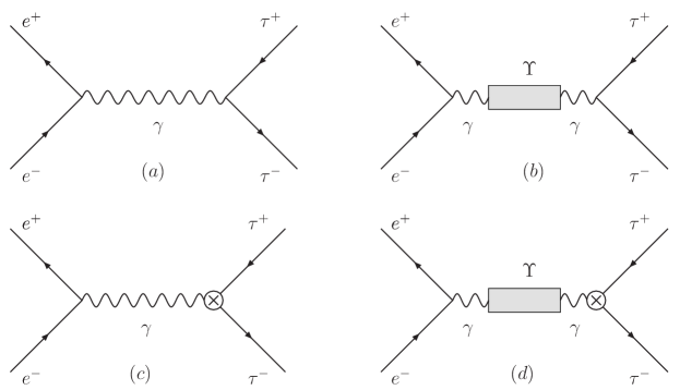
Figure 1: Diagrams (a) direct $\gamma$ exchange (b) $\Upsilon$ production (c) EDM in $\gamma$ exchange (d) EDM at the $\Upsilon$-peak.

3 Low energy polarized beams and the EDM.

As we will show, the EDM can be studied at leading order in the angular distribution of the $e^{+}e^{-}\longrightarrow\tau^{+}(s_{+})\tau^{-}(s_{-})$ differential cross section for longitudinally polarized electrons. The polarization of the final fermions is determined through the study of the angular distribution of their decay products. In our analysis we only keep linear terms in the EDM, neglecting terms proportional to the mass of the electron.

When considering the measurement of the polarization of just one of the taus, the normal -to the scattering plane- polarization ($P_{N}$) of each tau is the only component which is $T$-odd. For $CP$-conserving interactions, the $CP$-even term $(s_{+}+s_{-})_{N}$ of the normal polarization only gets contribution through the combined effect of both an helicity-flip transition and the presence of absorptive parts, which are both suppressed in the standard model. For a $CP$-violating interaction, such as an EDM, the $(s_{+}-s_{-})_{N}$ $CP$-odd term gets a non-vanishing value without the need of absorptive parts.

As $P_{N}$ is even under parity ($P$) symmetry, the observable sensitive to the EDM will need, in addition to $d_{\gamma}^{\tau}$, an additional $P$-odd contribution coming from longitudinally polarized electrons. A standard axial coupling, coming from a $Z$-exchange in the s-channel, could also be considered as an alternative but in that case the contribution is suppressed by powers of $\left(q^{2}/M_{Z}^{2}\right)$.

Following the notation of references [13] and [14], we now show how to measure the EDM using low energy $CP$-odd observables. Our aim is to identify genuine $CP$-odd observables that are linear in the EDM and not (additionally) suppressed by either $(q^{2}/M_{Z}^{2})$ or unitarity corrections.

In the center of mass (CM) reference frame we choose the coordinates as in Fig.(2). The $\mbox{\boldmath$s$}^{\pm}$ are the $\tau^{\pm}$ spin vectors in the $\tau^{\pm}$ rest system, $s_{\pm}=(0,s^{x}_{\pm},s^{y}_{\pm},s^{z}_{\pm})$. With this setting, polarization along the directions $x,y,z$ correspond to what is called transverse (T), normal (N) and longitudinal (L) polarizations, respectively.

We first consider the $\tau$-pair production in $e^{+}e^{-}$ collisions though direct $\gamma$ exchange (diagrams (a) and (c) in Fig. 1.). Next, we will show that the basic results of this section still hold for resonant $\Upsilon$ production.

Let us assume from now on that the tau production plane and direction of flight can be fully reconstructed. This can be done [15] if both $\tau$’s decay semileptonically. The differential cross section for $\tau$ pair production with polarized electrons with helicity $\lambda$ is:

$$\left.\frac{d\sigma}{d\Omega_{\tau^{-}}}\right|_{\lambda}=\left.\frac{d\sigma^{0}}{d\Omega_{\tau^{-}}}\right|_{\lambda}+\left.\frac{d\sigma^{S}}{d\Omega_{\tau^{-}}}\right|_{\lambda}+\ldots$$ (4)

The terms to be considered include contributions from leading order standard model and effective operator (EDM). The dots take account for higher order terms in the effective Lagrangian that are beyond experimental sensitivity and which are not considered in this paper.

The first term of Eq. (4) represents the $\tau$ spin-independent differential cross section. The second term $\displaystyle\left.\frac{d\sigma^{S}}{d\Omega_{\tau^{-}}}\right|_{\lambda}$ includes the linear terms in the spin of the $\tau$’s and has sensitivity to the EDM in their normal polarization:

$$\left.\frac{d\sigma^{S}}{d\Omega_{\tau^{-}}}\right|_{\lambda}=\frac{\alpha^{2}}{16\ s}\,\beta \left\{\lambda\left[(s_{-}+s_{+})_{x}X_{+}+(s_{-}+s_{+})_{z}Z_{+}+(s_{-}-s_{+})_{y}Y_{-}\right)]+\right.$$ (5)

$$\quad\left.(s_{-}-s_{+})_{x}X_{-}+(s_{-}-s_{+})_{z}Z_{-}\right\}$$

where

$$X_{+} = \frac{1}{\gamma}\sin\theta_{\tau^{-}},\qquad\qquad\qquad\qquad X_{-}=-\frac{1}{2}\sin(2\theta)\,\displaystyle\frac{2m_{\tau}}{e}{\mathrm{I}m}\left\{d_{\tau}^{\gamma}\right\},$$

$$Z_{+} = -\cos\theta_{\tau^{-}},\qquad\qquad\qquad\qquad Z_{-}=-\frac{1}{\gamma}\sin^{2}\theta\,\displaystyle\frac{2m_{\tau}}{e}{\mathrm{I}m}\left\{d_{\tau}^{\gamma}\right\},$$

$$Y_{-} = \gamma\beta^{2}\cos\theta_{\tau^{-}}\,\sin\theta_{\tau^{-}}\,\displaystyle\frac{2m_{\tau}}{e}{\mathrm{R}e}\left\{d_{\tau}^{\gamma}\right\}.$$ (6)

and $\alpha$ is the fine structure constant, $s=q^{2}$ is the squared CM energy and $\gamma=\frac{\sqrt{s}}{2m_{\tau}}$, $\beta=\sqrt{1-\frac{1}{\gamma^{2}}}$ are the dilation factor and $\tau$ velocity, respectively.

As can be seen in Eq.(6), the EDM is the leading contribution to the Normal Polarization of the single tau.

Figure 2: Coordinate system for $h^{\pm}$ production from the $\tau^{\pm}$

3.1 Single $tau$ normal polarization observable

We now show how to get an observable proportional to the EDM term from the Normal polarization of a single tau in the complete process

$$e^{+}e^{-}(pol)\rightarrow\gamma\rightarrow\tau^{+}\tau^{-}\rightarrow h^{+}\bar{\nu}_{\tau}h^{-}\nu_{\tau}$$

The cross section can be written as a function of the kinematical variables of the hadrons into which each tau decays [16] as:

$$d\sigma\left.\left(e^{+}e^{-}\rightarrow\gamma\rightarrow\tau^{+}\tau^{-}\rightarrow h^{+}\bar{\nu}_{\tau}h^{-}\nu_{\tau}\right)\right|_{\lambda}=4\,d\sigma\left.\left(e^{+}e^{-}\rightarrow\tau^{+}(\overrightarrow{n}_{+}^{*})\,\tau^{-}(\overrightarrow{n}_{-}^{*})\right)\right|_{\lambda}$$

$$\times\,Br(\tau^{+}\rightarrow h^{+}\bar{\nu}_{\tau})Br(\tau^{-}\rightarrow h^{-}\nu_{\tau})\frac{d\Omega_{h^{+}}}{4\pi}\,\frac{d\Omega_{h^{-}}}{4\pi}$$ (7)

with

$$\overrightarrow{n}_{\pm}^{*}=\mp\alpha_{\pm}\frac{\overrightarrow{q}^{*}_{\pm}}{\arrowvert\overrightarrow{q}^{*}_{\pm}\arrowvert}=\mp\alpha_{\pm}(\sin\theta_{\pm}^{*}\,\cos\phi_{\pm},\sin\theta_{\pm}^{*}\,\sin\phi_{\pm},\cos\theta_{\pm}^{*})\\$$

The linear terms in the spin of the taus depend on several kinematic variables that we have to take into account: the CM polar angle $\theta_{\tau^{-}}$ of production of the $\tau^{-}$ with respect to the electron, the azimuthal $\phi_{\pm}$ and polar $\theta^{*}_{\pm}$ angles of the produced hadrons $h^{\pm}$ ($\hat{q}^{*}_{\pm}$) in the $\tau^{\pm}$ rest frame (the * means that the quantity is given in the $\tau$ rest frame; see Fig.2). These angles appear in a different way on each term. The $\theta_{\tau^{-}}$ angle enters in the cross section as coefficients (of the $(s_{-}+s_{+})_{x}$ term, for example) while the hadron’s angles appear in the cross section through the polarization parameters $\overrightarrow{n}^{*}_{\pm}$. The whole angular dependence of each contribution is unique and it is this dependence that allows to select one of the terms in the cross section. Indeed, it is by an integration on the $\theta_{\tau^{-}}$ angle, followed by a dedicated integration on the hadronic angles, that one can select a polarization term and there, the contribution of the EDM.

For the Normal Polarization term this works as follows. The integration over the $\tau^{-}$ variables $d\Omega_{\tau^{-}}$ erases all the information on the $Z_{+}$ and $Y_{+}$ term of the cross section. Then, the cross section can be written only in terms of the surviving terms as:

$$\left.d^{4}\sigma^{S}\right|_{\lambda} = \frac{\pi^{2}\alpha^{2}\beta}{4\,s}\,Br(\tau^{+}\rightarrow h^{+}\bar{\nu}_{\tau})Br(\tau^{-}\rightarrow h^{-}\nu_{\tau})\,\frac{d\Omega_{h^{+}}}{4\pi}\,\frac{d\Omega_{h^{-}}}{4\pi}\,\times$$ (9)

$$\Bigg{\{}\frac{\lambda}{\gamma}\,\left[(n_{-}^{*})_{x}+(n_{+}^{*})_{x}\right]+\lambda\,\gamma\beta\,\left[(n_{-}^{*})_{y}-(n_{+}^{*})_{y}\right]\frac{2m_{\tau}}{e}\,{\mathrm{R}e}\left\{d^{\gamma}_{\tau}\right\}$$

$$+\frac{4}{3\gamma}\left[(n_{-}^{*})_{z}-(n_{+}^{*})_{z}\right]\frac{2m_{\tau}}{e}\,{\mathrm{I}m}\left\{d^{\gamma}_{\tau}\right\}\Bigg{\}}$$

As can be seen up to this point, helicity independent normal (longitudinal) polarization terms due to absorptive (EDM imaginary) parts may also survive. One may get rid of them by subtracting the cross sections for different helicities.

$$\left.\d^{2}\sigma^{S}\right|_{Pol(e^{-})}\equiv\left.d^{4}\sigma^{S}\right|_{\lambda=1}-\left.d^{4}\sigma^{S}\right|_{\lambda=-1}$$ (10)

Then, in order to enhance and select the corresponding $P_{N}$ observable, one has integrate as much as kinematic variables as possible without erasing the signal of the EDM (${\mathrm{R}e}\left\{d^{\gamma}_{\tau}\right\}\rightarrow d^{\gamma}_{\tau}$ from now on). Keeping only azimuthal angles and integrating all other variables one gets:

$$\left.\frac{d^{2}\sigma^{S}}{d\phi_{-}d\phi_{+}}\right|_{Pol(e^{-})} = \frac{\pi\alpha^{2}\beta}{32s}\,Br(\tau^{+}\rightarrow h^{+}\bar{\nu}_{\tau})Br(\tau^{-}\rightarrow h^{-}\nu_{\tau})\times$$ (12)

$$\Big{\{}\frac{1}{\gamma}\left[(\alpha_{-})\cos\phi_{-}-(\alpha_{+})\cos\phi_{+}\right]+$$

$$\beta\,\gamma\left[(\alpha_{-})\cos\phi_{-}-(\alpha_{+})\cos\phi_{+}\right]\frac{2m_{\tau}}{e}\,d^{\gamma}_{\tau}\Big{\}}$$

Now, to be sensitive only to the EDM we can define the azimuthal asymmetry as:

$$A_{N}^{\mp}=\frac{\sigma^{\mp}_{L}-\sigma^{\mp}_{R}}{\sigma}=\alpha_{\mp}\frac{3\pi\gamma\beta}{8(3-\beta^{2})}\frac{2m_{\tau}}{e}\,d^{\gamma}_{\tau}$$ (13)

where

$$\sigma^{\mp}_{L} = \int_{0}^{2\pi}d\phi_{\pm}\left[\int_{0}^{\pi}d\phi_{\mp}\,\left.\frac{d^{2}\sigma^{S}}{d\phi_{-}d\phi_{+}}\right|_{Pol(e^{-})}\right]=$$ (14)

$$\quad Br(\tau^{+}\rightarrow h^{+}\bar{\nu}_{\tau})Br(\tau^{-}\rightarrow h^{-}\nu_{\tau})\,\alpha_{\mp}\frac{(\pi\alpha\beta)^{2}\gamma}{8s}\,\frac{2m_{\tau}}{e}\,d^{\gamma}_{\tau}$$

$$\sigma^{\mp}_{R} = \int_{0}^{2\pi}d\phi_{\pm}\left[\int_{\pi}^{2\pi}d\phi_{\mp}\,\left.\frac{d^{2}\sigma^{S}}{d\phi_{-}d\phi_{+}}\right|_{Pol(e^{-})}\right]=$$ (15)

$$\quad-Br(\tau^{+}\rightarrow h^{+}\bar{\nu}_{\tau})Br(\tau^{-}\rightarrow h^{-}\nu_{\tau})\,\alpha_{\mp}\frac{(\pi\alpha\beta)^{2}\gamma}{8s}\,\frac{2m_{\tau}}{e}\,d^{\gamma}_{\tau}\$$

It is easy to verify that all other terms in the considered cross section are eliminated when we integrate in this way. Notice that this integration procedure does not erase contributions coming from the $CP$-even term of the Normal Polarization as it will be shown in the next section.

To get rid of $CP$-even terms one has to define a true $CP$ violation observable by summing up the defined asymmetry (13) for $\tau^{+}$ and for $\tau^{-}$

$$A_{N}^{CP}=\frac{1}{2}\left(A_{N}^{+}+A_{N}^{-}\right)=\alpha_{h}\frac{3\pi\gamma\beta}{8(3-\beta^{2})}\frac{2m_{\tau}}{e}\,d^{\gamma}_{\tau}$$ (16)

This observable is free of the CP-even contributions described in what follows and it is a genuine CP-odd observable.

3.2 $\gamma-Z$ interference

Contributions to this observable can also come from the standard $Z-\gamma$ interference:

$$\left.\frac{d\sigma^{0}}{d\Omega_{\tau^{-}}}\right|_{\lambda}^{Z\gamma} = \frac{\alpha^{2}|P_{Z}|^{2}}{16\ (2s_{w}c_{w})^{2}}\,\beta\,\left(s-M_{Z}^{2}\right)\,M^{Z\gamma}_{0}$$ (17)

$$\left.\frac{d\sigma^{S}}{d\Omega_{\tau^{-}}}\right|_{\lambda}^{Z\gamma} = \frac{\alpha^{2}|P_{Z}|^{2}}{16\ (2s_{w}c_{w})^{2}}\,\beta\left\{\Gamma_{Z}\,M_{Z}\left[(s_{-}+s_{+})_{y}Y_{+}^{Z\gamma}\right]+\right.$$ (18)

$$\left.\left(s-M_{Z}^{2}\right)\left[(s_{-}+s_{+})_{x}X^{Z\gamma}_{+}+(s_{-}+s_{+})_{z}Z^{Z\gamma}_{+}\right]+\right\}$$

where

$$|P_{Z}|^{2} = \frac{1}{(s-M_{Z}^{2})^{2}+\Gamma_{Z}^{2}M_{Z}^{2}},\quad a=-\frac{1}{2},\quad v=-\frac{1}{2}+2s_{w}^{2}$$

$$M_{0}^{Z\gamma} = \lambda\,a\,v(2\beta\cos\theta+2-\beta^{2}\sin^{\theta})-a^{2}\beta\cos\theta-v^{2}(2-\beta^{2}\sin^{2}\theta)$$

$$X_{+}^{Z\gamma} = \frac{1}{\gamma}\left[\lambda(2v^{2}+a^{2}\beta\cos\theta)-a\,v(2-\beta\cos\theta)\right]$$

$$Z^{Z\gamma}_{+} = \left[a^{2}\beta(1+\cos^{2}\theta)+2v^{2}\cos\theta\right]-a\,v\left[\beta(1+\cos^{2}\theta)+2\cos\theta\right]$$

$$Y_{+}^{Z\gamma} = \frac{1}{\gamma}a\,\beta(\lambda\,v-a)\sin\theta$$ (19)

Subtracting the cross sections for different helicities and integrating, as in the previous section, one gets

$${}^{Z\gamma}\sigma^{\mp}_{L} = \frac{\pi\alpha^{2}\beta}{2(2s_{w}c_{w})^{2}s}\,|P_{Z}|^{2}\,Br(\tau^{+}\rightarrow h^{+}\bar{\nu}_{\tau})Br(\tau^{-}\rightarrow h^{-}\nu_{\tau})\,a\,v\,\times$$ (20)

$$\quad\left\{4\left(s-M_{Z}^{2}\right)\left(1-\frac{\beta^{2}}{3}\right)\mp\alpha_{\mp}\Gamma_{Z}M_{Z}\frac{\pi\beta}{4\gamma}\right\}$$

$${}^{Z\gamma}\sigma^{\mp}_{R} = \frac{\pi\alpha^{2}\beta}{2(2s_{w}c_{w})^{2}s}\,|P_{Z}|^{2}\,Br(\tau^{+}\rightarrow h^{+}\bar{\nu}_{\tau})Br(\tau^{-}\rightarrow h^{-}\nu_{\tau})\,a\,v\,\times$$ (21)

$$\quad\left\{4\left(s-M_{Z}^{2}\right)\left(1-\frac{\beta^{2}}{3}\right)\pm\alpha_{\mp}\Gamma_{Z}M_{Z}\frac{\pi\beta}{4\gamma}\right\}$$

so that the $Z$ contribution to the asymmetry (13) is

$${}^{Z\gamma}A_{N}^{\mp}=\mp\alpha_{\mp}\frac{3\pi\beta\gamma}{8(3-\beta^{2})}\,\overbrace{\frac{a\,v}{\gamma^{2}(2s_{w}c_{w})^{2}}\frac{s\Gamma_{Z}M_{Z}}{(s-M_{Z}^{2})^{2}+(\Gamma_{Z}M_{Z})^{2}}}^{\varepsilon}$$ (22)

At 10 Gev, the value of the $\varepsilon$ factor is of the order $1\times 10^{-6}$, which makes this contribution to the asymmetry two orders of magnitude below the expected sensitivity for the EDM. Anyway, this asymmetry does not contribute to the $CP$-odd $A_{N}^{CP}$ of Eq.(16).

3.3 Observables at the $\Upsilon$ resonances

All these ideas can be applied for $e^{+}e^{-}$ collisions at the $\Upsilon$ peak where the $\tau$ pair production is mediated by the resonance: $e^{+}e^{-}\rightarrow\Upsilon\rightarrow\tau^{-}\tau^{-}$. At the $\Upsilon$ production energies we have an important tau pair production rate. We are interested in $\tau$ pairs produced by the decays of the $\Upsilon$ resonances, therefore we can use $\Upsilon(1S)$, $\Upsilon(2S)$ and $\Upsilon(3S)$ where the decay rates into tau pairs have been measured. At the $\Upsilon(4S)$ peak, although it decays dominantly into $B\overline{B}$, high luminosity B-Factories have an important direct tau pair production. Except for this last case, that can be studied with the results of the preceding sections, we assume that the resonant diagrams (b) and (d) of Fig. 1. dominate the process on the $\Upsilon$ peaks. This has been extensively discussed in ref.([17].

The main result is that the tau pair production at the $\Upsilon$ peak introduces the same tau polarization matrix terms as the direct production with $\gamma$ exchange (diagrams (a) and (c)). The only difference is an overall factor $|H(s)|^{2}$ in the cross section which is responsible for the enhancement at the resonant energies, the pure resonant (imaginary) amplitude being

$$H(M_{\Upsilon}^{2})=-i\,\frac{3}{\alpha}Br\left(\Upsilon\rightarrow e^{+}e^{-}\right)$$ (23)

Besides, it is easy to show that, at the $Upsilon$ peak, the interference of diagrams (a) and (d) plus the interference of diagrams (b) and (c) is exactly zero and so it is the interference of diagrams (a) and (b). Finally, the only contributions proportional to the EDM come with the interference of diagrams (b) and (d), while diagram (b) squared gives the leading contribution to the cross section.

The computations we did before can be repeated here, and finally we obtain no changes in the asymmetries: the only difference is in the value of the resonant production cross section at the $\Upsilon$ peak that is multiplied by the overall factor $|H(M_{\Upsilon}^{2})|^{2}$.

In fact, one can take the four diagrams (a,b,c,d) together and still get the same results we have already shown. Energies off or on the resonance will automatically select the significant diagrams.

4 Bounds on the EDM

We can now estimate the bounds on the EDM that can be achieved using this observable. For numerical results we assume a set of integrated luminosities for high statistics $B$/Flavor factories. We also consider the $\pi^{\pm}\;\bar{\nu_{\tau}}$ or $\rho^{\pm}\;\bar{\nu_{\tau}}$ (i.e. $h_{1},\;h_{2}=\pi,\;\rho$ ) decay channels for the traced $\tau^{\pm}$, while we sum up over $\pi^{\mp}\;\nu_{\tau}$ and $\rho^{\mp}\;\nu_{\tau}$ hadronic decay channels for the non traced $\tau^{\mp}$.

For comparison with other references, we show the bounds for the $\tau$-EDM that can be set in different scenarios:

$$|d^{\gamma}_{\tau}| \leq 4.4\ 10^{-19}\ ecm\quad\mbox{Babar + Belle at $2ab^{-1}$}$$

$$|d^{\gamma}_{\tau}| \leq 1.6\ 10^{-19}\ ecm\quad\mbox{Super B/Flavor factory, 1 yr running, $15ab^{-1}$}$$

$$|d^{\gamma}_{\tau}| \leq 7.2\ 10^{-20}\ ecm\quad\mbox{Super B/Flavor factory, 5 yrs running, $75ab^{-1}$}$$ (24)

These bounds improve present ones by 3 orders of magnitude.

We can also define other observables that are sensitive to the imaginary part of the EDM. The analysis is similar to the one we have done here and in ref.([17]).

To conclude, we have shown that low energy data makes possible a clear separation of the effects coming from the electromagnetic-EDM, the weak-EDM and interference effects. Polarized electron beams open the possibility to put bounds on the $\tau$ EDM looking at single tau polarization observables with low energy data. These observables allow for an independent analysis of the EDM bounds from what has been done with other high and low energy data.

References

• [1] W.-M. Yao et al., Journal of Physics G 33, (2006) 1; K.ย Inami et al. [BELLE Collaboration], Phys. Lett. B551 (2003) 16.
• [2] Y.ย Fukuda et al. [Super-Kamiokande Collaboration], Phys.ย Rev.ย Lett.ย 81 (1998) 1562.
• [3] J.ย Bernabรฉu, G.A.ย Gonzรกlez-Sprinberg and J.ย Vidal, Phys. Lett. B326 (1994) 168.
• [4] W.ย Bernreuther, U.ย Low, J.ย P.ย Ma and O.ย Nachtmann, Z.ย Phys.ย C 43, 117 (1989).
• [5] M. Acciarri et al. [L3 Collaboration], Phys. Lett. B434 (1998) 169.
• [6] D.ย Buskulic et al. [ALEPH Collaboration], Phys.ย Lett.ย B 346, 371 (1995); K.ย Ackerstaff et al. [OPAL Collaboration], Z.ย Phys.ย C 74, 403 (1997); H.Albrecht et al. [ARGUS Collaboration], Phys. Lett. B485 (2000) 37.
• [7] F. del Aguila and M. Sher, Phys. Lett. B252 (1990) 116.
• [8] J.A. Grifols and A. Mendez, Phys. Lett. B255 (1991) 611 and Erratum Phys. Lett. B259 (1991) 512.
• [9] R. Escribano and E. Masso, Phys. Lett. 395 (1997) 369.
• [10] B. Ananthanarayan and S.D. Rindani, Phys. Rev. D51 (1995) 5996
• [11] See for example http://www.lnf.infn.it/conference/superb06/ and http://www-conf.slac.stanford.edu/superb/.
• [12] W.ย Buchmuller and D.ย Wyler, Nucl. Phys. B268 (1986) 621; C.N.ย Leung, S.T.ย Love and S.ย Rao, Zeit. fรผr Physik C31 (1986) 433; M. Bilenky and A. Santamaria, Nucl. Phys. B420 (1994) 47.
• [13] G.A.ย Gonzรกlez-Sprinberg, A.ย Santamaria, J.ย Vidal, Nucl. Phys. B582 (2000) 3.
• [14] J.ย Bernabรฉu, G.A.ย Gonzรกlez-Sprinberg, M.ย Tung and J.ย Vidal, Nucl. Phys. B436 (1995) 474.
• [15] J.ย H.ย Kuhn, Phys.ย Lett.ย B 313 (1993) 458.
• [16] Y.S.ย Tsai Phys. Rev. D4 (1971) 2821.
• [17] J.ย Bernabeu, G.ย A.ย Gonzalez-Sprinberg and J.ย Vidal, Nucl.ย Phys.ย B 701(2004) 87.