MSSM flat direction inflation: slow roll, stability, fine tunning and reheating

Abstract:

We consider low scale slow roll inflation driven by the gauge invariant flat directions udd and LLe of the Minimally Supersymmetric Standard Model at the vicinity of a saddle point of the scalar potential. We study the stability of saddle point and the slow roll regime by considering radiative and supergravity corrections. The latter are found to be harmless, but the former require a modest finetuning of the saddle point condition. We show that while the inflaton decays almost instantly, full thermalization occurs late, typically at a temperature $T\approx 10^{7}$ GeV, so that there is no gravitino problem. We also compute the renormalization group running of the inflaton mass and relate it to slepton masses that may be within the reach of LHC and could be precisely determined in a future Linear Collider experiment.

1 Introduction

Recently we have constructed a model of inflation [1] based on the udd and LLe flat directions of Minimally Supersymmetric Standard Model (MSSM; for a review of MSSM flat directions, see [2]). In this model the inflaton is a gauge invariant combination of either squark or slepton fields. For a choice of the soft SUSY breaking parameters $A$ and the inflaton mass $m_{\phi}$, the potential along the flat udd and LLe directions is such that there is a period of slow roll inflation of sufficient duration to provide the observed spectrum of CMB perturbations. In the inflationary part of the MSSM potential the second derivative is vanishing and the slow roll phase is driven by the third derivative of the potential .

MSSM inflation occurs at a very low scale with $H_{inf}\sim 1-10$ GeV and with field values much below the Planck scale. Hence it stands in strong contrast to the conventional inflation models which are based on ad hoc gauge singlet fields and often employ field values close to Planck scale (for a review, see  [4]). In such models the inflaton couplings to SM physics are unknown. As a consequence, much of the post-inflationary evolution, such as reheating, thermalization, generation of baryon asymmetry and cold dark matter, which all depend very crucially on how the inflaton couples to the (MS)SM sector [5, 6, 7, 8], is not calculable from first principles. The great virtue of MSSM inflation based on flat directions is that the inflaton couplings to Standard Model particles are known and, at least in principle, measurable in laboratory experiments such as LHC or a future Linear Collider.

However, as in almost all inflationary models, a fine tuning of the initial condition is needed to place the flat direction field $\phi$ to the immediate vicinity of the saddle point $\phi_{0}$ at the onset of inflation. In addition, there is the question of the stability of the saddle point solution and of the existence of a slow roll regime. These are issues that we wish to address in detail in the present paper. Both supergravity and radiative corrections to the flat direction inflaton potential must be considered. Hence we need to write down and solve the renormalization group (RG) equations for the MSSM flat directions of interest. RG equations are also needed to scale the model parameters, such as the inflaton mass, down to TeV scale; since the inflaton mass is related either to squark or slepton masses, it could be measured by LHC or a future Linear Collider.

Because the inflaton couplings to ordinary matter are known, inflaton decay and thermalization are processes that can be computed in an unambiguous way. Unlike in many models with a singlet inflaton, in MSSM inflation the potential relevant for decay and thermalization cannot be adjusted independently of the slow roll part of the potential.

This paper is organized as follows. In Sect. 2 we present the model of MSSM inflation and its predictions. In Sect. 3 we study the flat direction potential without an exact saddle point. We find generic constraints for the existence of a slow roll solution and show that in the slow roll regime there is always tunneling from a false minimum. In Sect. 4 we solve the one-loop RG equations for the LLe flat direction and find the one-loop corrected saddle point. We quantify the amount of fine tuning required for the slow roll solution to exist, and relate through RG running the LLe inflaton mass with observables such as the slepton masses at the LHC energy scale. We also show that supergravity corrections to the potential can be neglected. In Sect. 5 we discuss the decay of the flat direction, the reheating and thermalization of the Universe, and show that the reheat temperature is low enough for the model to avoid the gravitino problem. Sect. 6 contains our conclusions and some discussion about future prospects.

2 The Model

Let us recapitulate the main features of MSSM flat direction inflation [1]. As is well known, in the limit of unbroken SUSY the flat directions have exactly vanishing potential. This situation changes if we take into account soft SUSY breaking and non-renormalizable superpotential terms  of the type [2]

$$W_{non}=\sum_{n>3}{\lambda_{n}\over n}{\Phi^{n}\over M^{n-3}}\,,$$ (1)

where $\Phi$ is a superfield which contains the flat direction. Within MSSM all the flat directions are lifted by non-renormalizable operators with $4\leq n\leq 9$ [11], where $n$ depends on the flat direction. We expect that quantum gravity effects yield $M=M_{\rm P}=2.4\times 10^{18}$ GeV and $\lambda_{n}\sim{\cal O}(1)$ [12] .

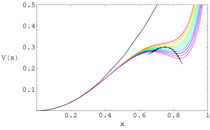
Figure 1: The colored curves depict the full potential, where $V(x)\equiv V(\phi)/(0.5~{}m_{\phi}^{2}M_{\rm P}^{2}(m_{\phi}/M_{\rm P})^{1/2})$, and $x\equiv(\lambda_{n}M_{\rm P}/m_{\phi})^{1/4}(\phi/M_{\rm P})$. The black curve is the potential arising from the soft SUSY breaking mass term. The black dots on the colored potentials illustrate the gradual transition from minimum to the saddle point and to the maximum.

Let us focus on the lowest order superpotential term in Eq. (1) which lifts the flat direction. Soft SUSY breaking induces a mass term for $\phi$ and an $A$-term so that the scalar potential along the flat direction reads

$$V={1\over 2}m^{2}_{\phi}\,\phi^{2}+A\cos(n\theta+\theta_{A}){\lambda_{n}\phi^{n}\over n\,M^{n-3}_{\rm P}}+\lambda^{2}_{n}{{\phi}^{2(n-1)}\over M^{2(n-3)}_{\rm P}}\,,$$ (2)

Here $\phi$ and $\theta$ denote respectively the radial and the angular coordinates of the complex scalar field $\Phi=\phi\,\exp[i\theta]$, while $\theta_{A}$ is the phase of the $A$-term (thus $A$ is a positive quantity with dimension of mass). Note that the first and third terms in Eq. (2) are positive definite, while the $A$-term leads to a negative contribution along the directions whenever $\cos(n\theta+\theta_{A})<0$. 

In principle, in the $A$-term all the superpotential terms of a given dimension $n$ may enter with a different coefficient $A_{n}$; whether they are related or not depends on the details of the SUSY breaking mechanism.

2.1 The Saddle Point

The maximum impact from the $A$-term is obtained when $\cos(n\theta+\theta_{A})=-1$ (which occurs for $n$ values of $\theta$). Along these directions $V$ has a secondary minimum at $\phi=\phi_{0}\sim\left(m_{\phi}M^{n-3}_{\rm P}\right)^{1/n-2}\ll M_{\rm P}$ (the global minimum is at $\phi=0$), provided that

$$A^{2}\geq 8(n-1)m^{2}_{\phi}\,.$$ (3)

At this minimum the curvature of the potential is positive both along the radial and angular directions with $V\sim m_{\phi}^{2}\phi_{0}^{2}\sim m_{\phi}^{2}\left(m_{\phi}M^{n-3}_{\rm P}\right)^{2/(n-2)}$.

As discussed in  [1], if the local minimum is too steep, the field will become trapped there with an ensuing inflation that has no graceful exit like in the old inflation scenario [14]. On the other hand in an opposite limit, with a point of inflection, a single flat direction cannot support inflation [15].

However, in the gravity mediated SUSY breaking case, the $A$-term and the soft SUSY breaking mass terms are expected to be the same order of magnitude as the gravitino mass, i.e.

$$m_{\phi}\sim A\sim m_{3/2}\sim{\cal O}(1)~{}{\rm TeV}\,.$$ (4)

Therefore, as pointed out in [1], in the gravity mediated SUSY breaking it is possible that the potential barrier actually disappears and the inequality in Eq. (3) is saturated so that $A$ and $m_{\phi}$ are related by

$$A^{2}=8(n-1)m^{2}_{\phi}\,.$$ (5)

This represents a fine tuning and will be discussed at length in the next Sections. However, let us now assume for the sake of argument that Eq. (5) holds. Then both the first and second derivatives of $V$ vanish at $\phi_{0}$,  i.e. $V^{\prime}(\phi_{0})=0,~{}V^{\prime\prime}(\phi_{0})=0$. As the result, if initially $\phi\sim\phi_{0}$, a slow roll phase of inflation is driven by the third derivative of the potential.

Note that this behavior does not seem possible for other SUSY breaking scenarios such as the gauge mediated breaking [16] or split SUSY [17]. In split SUSY the $A$-term is protected by an $R$-symmetry, which also keeps the gauginos light while the sfermions are quite heavy [17] .

2.2 Slow roll

The potential near the saddle point Eq. (5) is very flat along the real direction but not along the imaginary direction. Along the imaginary direction the curvature is determined by $m_{\phi}$. Around $\phi_{0}$ the field lies in a plateau with a potential energy

$$V(\phi_{0})={(n-2)^{2}\over 2n(n-1)}\,m^{2}_{\phi}\phi_{0}^{2}$$ (6)

with

$$\phi_{0}=\left({m_{\phi}M^{n-3}_{\rm P}\over\lambda_{n}\sqrt{2n-2}}\right)^{1/(n-2)}\,.$$ (7)

This results in Hubble expansion rate during inflation which is given by

$$H_{\rm inf}={(n-2)\over\sqrt{6n(n-1)}}{m_{\phi}\phi_{0}\over M_{\rm P}}.$$ (8)

When $\phi$ is very close to $\phi_{0}$, the first derivative is extremely small. The field is effectively in a de Sitter background, and we are in self-reproduction (or eternal inflation) regime where the two point correlation function for the flat direction fluctuation grows with time. But eventually classical friction wins and slow roll begins at $\phi\approx\phi_{\rm self}$ [1]

$$(\phi_{0}-\phi_{\rm self})\simeq\Big{(}{m_{\phi}\phi_{0}^{2}\over M_{\rm P}^{3}}\Big{)}^{1/2}\phi_{0}.$$ (9)

The slow roll potential in this case reads

$$V(\phi)=V(\phi_{0})+{1\over 3!}V^{\prime\prime\prime}(\phi_{0})(\phi-\phi_{0})^{3}+\cdot\cdot\cdot\,,$$

$$V^{\prime\prime\prime}({\phi_{0}})=2(n-2)^{2}{m^{2}_{\phi}\over\phi_{0}}\,.$$ (10)

We can now solve the equation of motion for the $\phi$ field in the slow-roll approximation,

$$3H\dot{\phi}=-\frac{1}{2}V^{\prime\prime\prime}(\phi_{0})(\phi-\phi_{0})^{2}\,,$$ (11)

assuming initial conditions such that the flat direction starts in the vicinity of $\phi_{0}$ with $\dot{\phi}\approx 0$. Inflation ends when the slow roll parameter, $\epsilon\equiv(M_{\rm P}^{2}/2)(V^{\prime}/V)^{2}$ becomes of ${\cal O}(1)$. This occurs at

$$(\phi_{0}-\phi_{\rm end})\sim{\phi^{3}_{0}\over 2n(n-1)M^{2}_{\rm P}}\,.$$ (12)

which happens to be also the place when the other slow roll paremeter $\eta\equiv M^{2}_{\rm P}(V^{\prime\prime}/V)$ becomes of ${\cal O}(1)$.

The number of e-foldings during the slow roll from $\phi$ to $\phi_{\rm end}$ is given by

$${\cal N}_{e}(\phi)=\int_{\phi}^{\phi_{\rm end}}{H_{\rm inf}d\phi\over\dot{\phi}}\simeq{\phi^{3}_{0}\over 2n(n-1)M^{2}_{\rm P}(\phi_{0}-\phi)}\,,$$ (13)

where we have used $V^{\prime}(\phi)\sim(\phi-\phi_{0})^{2}V^{\prime\prime\prime}(\phi_{0})$ (this is justified since $V^{\prime}(\phi_{0})\sim 0,V^{\prime\prime}(\phi_{0})\sim 0$), and Eq. (11). The total number of e-foldings in the slow roll regime is then found from Eq.(9)

$${\cal N}_{\rm tot}\simeq{1\over 2n(n-1)}\big{(}{\phi^{2}_{0}\over m_{\phi}M_{\rm P}}\Big{)}^{1/2}.$$ (14)

The observationally relevant perturbations are generated when $\phi\approx\phi_{\rm COBE}$. The number of e-foldings between $\phi_{\rm COBE}$ and $\phi_{\rm end}$, denoted by ${\cal N}_{\rm COBE}$ follows from Eq. (13)

$${\cal N}_{\rm COBE}\simeq{\phi^{3}_{0}\over 2n(n-1)M^{2}_{\rm P}(\phi_{0}-\phi_{\rm COBE})}.$$ (15)

The amplitude of perturbations thus produced is given by

$$\delta_{H}\equiv\frac{1}{5\pi}\frac{H^{2}_{\rm inf}}{\dot{\phi}}\simeq\frac{1}{5\pi}\sqrt{\frac{2}{3}n(n-1)}(n-2)~{}\Big{(}{m_{\phi}M_{\rm P}\over\phi_{0}^{2}}\Big{)}~{}{\cal N}_{\rm COBE}^{2},$$ (16)

where we have used Eqs.(8), (2.2), (15). Again after using these equations, the spectral tilt of the power spectrum and its running are found to be

$$n_{s}=1+2\eta-6\epsilon\ \simeq\ 1-{4\over{\cal N}_{\rm COBE}}\,,$$ (17)

$${d\,n_{s}\over d\ln k}=-{4\over{\cal N}_{\rm COBE}^{2}}.\,$$ (18)

2.3 Properties and predictions

As discussed in [1], among the about 300 flat directions there are two that can lead to a successful inflation along the lines discussed above.

One is udd which, up to an overall phase factor, is parameterized by

$$u^{\alpha}_{i}=\frac{1}{\sqrt{3}}\phi\,,~{}d^{\beta}_{j}=\frac{1}{\sqrt{3}}\phi\,,~{}d^{\gamma}_{k}=\frac{1}{\sqrt{3}}\phi\,.$$ (19)

Here $1\leq\alpha,\beta,\gamma\leq 3$ are color indices, and $1\leq i,j,k\leq 3$ denote the quark families. The flatness constraints require that $\alpha\neq\beta\neq\gamma$ and $j\neq k$.

The other direction is LLe, parameterized by (again up to an overall phase factor)

$$L^{a}_{i}=\frac{1}{\sqrt{3}}\left(\begin{array}[]{l}0\\ \phi\end{array}\right)\,,~{}L^{b}_{j}=\frac{1}{\sqrt{3}}\left(\begin{array}[]{l}\phi\\ 0\end{array}\right)\,,~{}e_{k}=\frac{1}{\sqrt{3}}\phi\,,$$ (20)

where $1\leq a,b\leq 2$ are the weak isospin indices and $1\leq i,j,k\leq 3$ denote the lepton families. The flatness constraints require that $a\neq b$ and $i\neq j\neq k$. Both these flat directions are lifted by $n=6$ non-renormalizable operators,

$$W_{6}\supset\frac{1}{M_{\rm P}^{3}}(LLe)(LLe)\,,\hskip 28.45274ptW_{6}\supset\frac{1}{M_{\rm P}^{3}}(udd)(udd)\,.$$ (21)

The reason for choosing either of these two flat directions is twofold: (i) a non-trivial $A$-term arises, at the lowest order, only at $n=6$; and (ii) we wish to obtain the correct COBE normalization of the CMB spectrum.

Those MSSM flat directions which are lifted by operators with dimension $n=7,9$ are such that the superpotential term contains at least two monomials, i.e. is of the type

$$W\sim\frac{1}{M_{\rm P}^{n-3}}\Psi\Phi^{n-1}\,.$$ (22)

If $\phi$ represents the flat direction, then its VEV induces a large effective mass term for $\psi$, through Yukawa couplings, so that $\langle\psi\rangle=0$. Hence Eq. (22) does not contribute to the $A$-term.

More importantly, as we will see, all other flat directions except those lifted by $n=6$ fail to yield the right amplitude for the density perturbations. Indeed, as can be seen in Eq. (7), the value of $\phi_{0}$, and hence also the energy density, depend on $n$.

According to the arguments presented above, successful MSSM flat direction inflation has the following model parameters:

$$m_{\phi}\sim 1-10~{}{\rm TeV}\,,~{}~{}n=6\,,~{}~{}A=\sqrt{40}m_{\phi}\,,~{}~{}\lambda\sim{\cal O}(1)\,.$$ (23)

Here we assume that $\lambda$ (we drop the subscript ”6”) is of order one, which is the most natural assumption when $M=M_{\rm P}$.

The Hubble expansion rate during inflation and the VEV of the saddle point are 

$$H_{\rm inf}\sim 1-10~{}{\rm GeV}\,,~{}~{}~{}\phi_{0}\sim(1-3)\times 10^{14}~{}{\rm GeV}\,.$$ (24)

Note that both the scales are sub-Planckian. The total energy density stored in the inflaton potential is $V_{0}\sim 10^{36}-10^{38}~{}{\rm GeV}^{4}$. The fact that $\phi_{0}$ is sub-Planckian guarantees that the inflationary potential is free from the uncertainties about physics at super-Planckian VEVs. The total number of e-foldings during the slow roll evolution is large enough to dilute any dangerous relic away, see Eq. (14):

$${\cal N}_{\rm tot}\sim 10^{3}\,,$$ (25)

Domains which are initially closer than $\phi_{\rm self}$ to $\phi_{0}$, see Eq. (9), can enter self-reproduction in eternal inflation, with no observable consequences.

At such low scales as in MSSM inflation the number of e-foldings, ${\cal N}_{\rm COBE}$, required for the observationally relevant perturbations, is much less than $60$ [20]. If the inflaton decays immediately after the end of inflation, we obtain ${\cal N}_{\rm COBE}\sim 50$. Despite the low scale, the flat direction can generate adequate density perturbations as required to explain the COBE normalization. This is due to the extreme flatness of the potential (recall that $V^{\prime}=0$), which causes the velocity of the rolling flat direction to be extremely small. From Eq. (16) we find an amplitude of

$$\delta_{H}\simeq 1.91\times 10^{-5}\,.$$ (26)

There is a constraint on the mass of the flat direction from the amplitude of the CMB anisotropy:

$$m_{\phi}\simeq(100~{}{\rm GeV})\times\lambda^{-1}\,\left(\frac{{\cal N}_{\rm COBE}}{50}\right)^{-4}\,.$$ (27)

We get a lower limit on the mass parameter when $\lambda\leq 1$. For smaller values of $\lambda\ll 1$, the mass of the flat direction must be larger. Note that the above bound on the inflaton mass arises at high scales, i.e. $\phi=\phi_{0}$. However, through renormalization group flow, it is connected to the low scale mass, as will be discussed in Sect. 4.

The spectral tilt of the power spectrum is not negligible because, although the first slow roll parameter is $\epsilon\sim 1/{\cal N}_{\rm COBE}^{4}\ll 1$, the other slow roll parameter is given by $\eta=-2/{\cal N}_{\rm COBE}$ and thus, see Eq. (17)

$$n_{s}\sim 0.92\,,$$ (28)

$${d\,n_{s}\over d\ln k}\sim-0.002\,,$$ (29)

where we have taken ${\cal N}_{\rm COBE}\sim 50$ (which is the maximum value allowed for the scale of inflation in our model). In the absence of tensor modes, this agrees with the current WMAP 3-years’ data within $2\sigma$ [22]. Note that MSSM inflation does not produce any large stochastic gravitational wave background during inflation. Gravity waves depend on the Hubble expansion rate, and in our case the energy density stored in MSSM inflation is very small.

3 Sensitivity of the saddle point inflation

In previous Sections and in Ref. [1] the dynamics of the flat direction inflaton was discussed assuming the saddle point condition Eq. (5) is satisfied exactly. The question then is, how large a deviation can be allowed for before slow roll inflation will be spoiled. There are obviously two distinct possibilities: either $A>\sqrt{8(n-1)}m_{\phi}$ or $A<\sqrt{8(n-1)}m_{\phi}$. (Although we always take $n=6$ in the present paper, we keep $n$ here for generality of the formalism.) In the former case there is a barrier which separates the global minimum $\phi=0$ and the false minimum at $\phi\simeq\phi_{0}$. The eventual inflationary trajectory starts near the top of the barrier. The field can either start at the top, or jump to its vicinity from the false minimum via Coleman-de Luccia tunneling [23]. As we will see, if the barrier is too high, there will be no inflation near the top. In the latter case there is no minimum but the potential may be too steep for slow roll inflation. Therefore we need to analyze the two cases separately. However, the steepness of the potential is a problem which is common to both cases and is addressed at the end of this Section.

To facilitate the discussion, let us define

$$\delta\equiv{A^{2}\over 8(n-1)m_{\phi}^{2}}\equiv 1\pm\left({n-2\over 2}\right)^{2}\,\alpha^{2}\,.$$ (30)

Here we will assume that $\alpha\ll 1$. Before beginning the calculations, we would like to point that the main results of this section are summarized in Fig. (3) and Eq. (60). These yield no constraint on the spectral tilt as any value consistent with sufficient slow roll inflation (i.e. a number $\geq{\cal N}_{\rm COBE}$ of e-foldings) is allowed.

3.1 The potential for $\delta>1$

In this case there are two extrema, a maximum $(-)$ and a minimum $(+)$,

$$\phi_{\pm}=\phi_{0}\,\left[\sqrt{\delta}\pm\sqrt{\delta-1}\right]^{1\over n-2}=\phi_{0}\left(1\pm{\alpha\over 2}+{\cal O}(\alpha^{2})\right)\,,$$ (31)

and a point of inflection $\phi_{i}$

$$\phi_{i}=\phi_{0}\Big{(}1+{n-2\over 32}\alpha^{2}+{\cal O}(\alpha^{4})\Big{)}.$$ (32)

We can then express the potential and its derivatives at the extrema $\phi_{-}$ and $\phi_{+}$ as functions of $\alpha$,

$$V(\phi_{\pm})=V(\phi_{0})\left(1-{n-1\over 2}\alpha^{2}\pm{n(n-1)\over 6}\alpha^{3}\right)\,,$$ (33)

$$V^{\prime\prime}(\phi_{\pm})=\pm\alpha(n-2)^{2}m_{\phi}^{2}\,,$$ (34)

$$V^{\prime\prime\prime}(\phi_{\pm})=V^{\prime\prime\prime}(\phi_{0})\left(1\pm{3\over 2}(n-2)\alpha\right)\,.$$ (35)

Note that $\alpha\to 0$ when $\delta\to 1$, so we can expand the potential around the maximum, and include the small $\alpha$ correction due to deviations from the saddle point as

$$V(\phi)=(n-2)^{2}m_{\phi}^{2}\phi_{0}^{2}\left[{1\over 2n(n-1)}-{\alpha\over 2}\left({\phi\over\phi_{0}}-1+{\alpha\over 2}\right)^{2}+{1\over 3}\left({\phi\over\phi_{0}}-1+{\alpha\over 2}\right)^{3}\right]\,.$$ (36)

The maximum is now at $\phi_{\rm max}=\phi_{0}(1-\alpha/2)$, and the minimum is at $\phi_{\rm min}=\phi_{0}(1+\alpha/2)$, with masses (curvature of the potential) given by $m^{2}_{\pm}=\pm(n-2)^{2}m_{\phi}^{2}\,\alpha$, which coincides with Eq. (34), while there is now a point of inflection at $\phi_{0}$. Note that the difference in potential height between the maximum and the minimum is

$${\Delta V\over V_{0}}={V_{\rm max}-V_{\rm min}\over V(\phi_{0})}={n(n-1)\over 3}\alpha^{3}\,.$$ (37)

In the limit of $\alpha\to 0$ we recover the saddle point. We will work in the limit when $\alpha\ll 1$.

Let us now define a few variables, $x=\phi/\phi_{0}$, $\,\tau=(n-2)m_{\phi}t$  and  $h=H_{\rm inf}/(n-2)m_{\phi}$. Then the equation of motion for the scalar field down the potential can be written as

$$x^{\prime\prime}+3hx^{\prime}+V^{\prime}(x)=x^{\prime\prime}+3hx^{\prime}+\Big{(}x-1+{\alpha\over 2}\Big{)}^{2}-\alpha\Big{(}x-1+{\alpha\over 2}\Big{)}=0\,,$$ (38)

where we have used (36).

The eventual inflationary trajectory will start in the vicinity of the maximum $x=1-\alpha/2$ and will roll down the hill towards $x=0$. The field can either start near the maximum, or tunnel to its vicinity out of the false vacuum. Tunneling takes place in the presence of a non-zero vacuum energy, $H_{\rm inf}\neq 0$, and is known as Coleman-de Luccia tunneling [23].

In order to find the interpolating solution between the false and the true vacuum one solves the Euclidean equation of motion,

$$x^{\prime\prime}+3hx^{\prime}-V^{\prime}(x)=x^{\prime\prime}+3hx^{\prime}-\Big{(}x-1+{\alpha\over 2}\Big{)}^{2}+\alpha\Big{(}x-1+{\alpha\over 2}\Big{)}=0\,,$$ (39)

whose exact solution is

$$x(\tau)=1-{\alpha\over 2}\tanh{\alpha\tau\over 6h}\,.$$ (40)

This solution starts at $x(-\infty)=1+\alpha/2=\phi_{+}/\phi_{0}$ and ends at $x(\infty)=1-\alpha/2=\phi_{-}/\phi_{0}$. The “tunneling” from $\phi_{\rm min}$ to $\phi_{\rm max}$ can actually be understood as diffusion due to de Sitter fluctuations. It is valid so long as $V^{\prime\prime}(\phi_{\rm min})\ll H^{2}_{\rm inf}$. This requires that, see Eq. (34),

$$\alpha\ll{1\over 6n(n-1)}{\phi_{0}^{2}\over M_{\rm P}^{2}}\,.$$ (41)

This also insures that $|\eta|\ll 1$ at the maximum, and hence inflation can take place after tunneling. Otherwise there will be no inflation, neither in self-reproduction nor in slow roll regime.

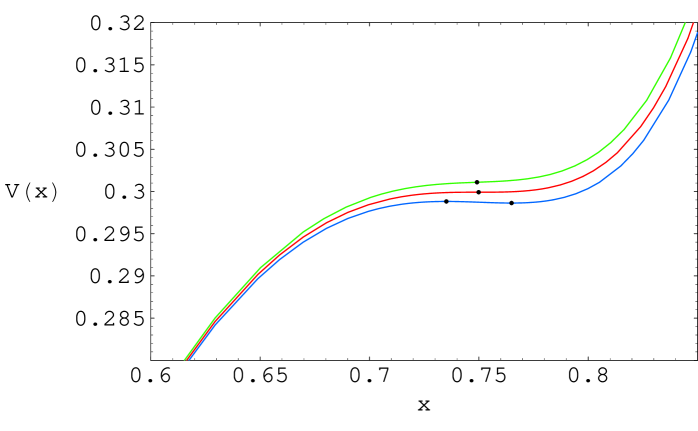
Figure 2: The red curve depicts the potential, $V(x)\equiv V(\phi)/(0.5m_{\phi}^{2}M_{\rm P}^{2}(m_{\phi}/M_{\rm P})^{1/2})$, where $x\equiv(\lambda_{n}M_{\rm P}/m_{\phi})^{1/4}(\phi/M_{\rm P})$, for the saddle point (shown by the black dot) when $\delta=1$. The blue curve illustrates the potential when $\delta=1+\sqrt{40}/1000$, where the two black dots, one on right shows the minimum value $\phi_{-}$ and on the left shows the maximum value, $\phi_{+}$. The green curve portrays the potential for the opposite case when $\delta=1-\sqrt{40}/1000$. The black dot is the point of inflection.

Let us now discuss the effect of the tunneling solutions on the tilt of the CMB spectrum. Again there is self-reproduction close to the maximum as long as the curvature there is smaller than the rate of expansion squared, i.e. $\alpha\ll 1/180(\phi_{0}/M_{\rm P})^{2}$. The slow-roll regime starts at $\phi\approx\phi_{\rm self}$ when

$$|(\phi_{\rm self}-\phi_{-})(\phi_{\rm self}-\phi_{+})|\leq{m_{\phi}\phi_{0}^{4}\over M_{\rm P}^{3}}\,,$$ (42)

Note that $|(\phi_{\rm self}-\phi_{-})|\simeq\ |(\phi_{+}-\phi_{-})|=\alpha\phi_{0}$, see Eq. (33), and $|(\phi_{\rm self}-\phi_{+})|\simeq|(\phi_{\rm self}-\phi_{0})|$. We therefore find

$$(\phi_{0}-\phi_{\rm self})\simeq{m_{\phi}\phi^{4}_{0}\over\alpha M^{3}_{\rm P}}.$$ (43)

Now we integrate Eq. (38) in the slow-roll approximation, using a new variable $u=x-x_{-}$, for which the equation of motion becomes $3hu^{\prime}=-u(u-\alpha)$. The exact solution is, in terms of the number of $e$-folds, ${\cal N}=h\tau$,

$$x({\cal N})=1-{\alpha\over 2}\,\coth(\beta{\cal N})$$ (44)

where we have defined

$$\beta={\alpha\over 6h^{2}}=n(n-1)\,\alpha\,{M_{\rm P}^{2}\over\phi_{0}^{2}}\,.$$ (45)

Note that in the limit $\alpha\to 0$, we recover the usual expression Eq. (13). From Eqs. (12), (43), (44), it turns out that the number of e-folds from $\phi_{\rm self}$ to the end of inflation at $\phi_{\rm end}$ is again of order $10^{3}$.

The required number of e-folds for the relevant perturbations (${\cal N}_{\rm COBE}\sim 50$) determines the value of $\phi_{\rm COBE}$,

$$|(\phi_{\rm COBE}-\phi_{-})(\phi_{\rm COBE}-\phi_{+})|^{1/2}={\alpha\over 2\sinh\beta{\cal N}}\simeq{3h^{2}\phi_{0}\over{\cal N}_{\rm COBE}}={\phi_{0}^{3}\over 2n(n-1)M_{\rm P}^{2}\,{\cal N}_{\rm COBE}}\,.$$ (46)

On the other hand, the amplitude of fluctuations is given by

$$\delta_{H}\simeq{3\over 5\pi}\,{H_{\rm inf}^{3}\over V^{\prime}(\phi)}={(n-2)\sqrt{n}\,(2n-2)^{n\over 2n-4}\over 5\pi\sqrt{3}}\,\lambda_{n}^{2\over n-2}\,\left({m_{\phi}\over M_{\rm P}}\right)^{n-4\over n-2}\,{\sinh^{2}\beta{\cal N}\over\beta^{2}}$$ (47)

which for $n=6,4,3$ becomes

$$\delta_{H}(n=6)\simeq 2\,\left({\lambda_{n}m_{\phi}\over M_{\rm P}}\right)^{1/2}\,{\sinh^{2}\beta{\cal N}\over\beta^{2}}\,,$$

$$\delta_{H}(n=4)\simeq\lambda_{n}\,{\sinh^{2}\beta{\cal N}\over\beta^{2}}\,,$$ (48)

$$\delta_{H}(n=3)\simeq 0.5\,\lambda_{n}^{2}{M_{\rm P}\over m_{\phi}}\,{\sinh^{2}\beta{\cal N}\over\beta^{2}}\,,$$

while the spectral tilt and its running are universal,

$$n_{s}=1-{d\ln\delta_{H}^{2}\over d{\cal N}}=1-4\beta\,\coth\beta{\cal N}\,,$$ (50)

$${d\,n_{s}\over d\,\ln k}=-{d\,n_{s}\over d{\cal N}}=-{4\beta^{2}\over\sinh^{2}\beta{\cal N}}\,,$$

which reduce to the usual expressions in the limit $\beta\to 0$, see Eqs. (17), (18). We show in Fig. 3 the variation of the tilt with $\beta$ for a model with ${\cal N}_{\rm COBE}=50$. Note that the range of allowed values of $\beta$ is constrained by the condition to have inflation near the maximum, i.e. that $|\eta|<1$ at $\phi_{-}$. This gives $\beta<0.06$, for $n=6$, see Eqs. (41,45). The corresponding range of tilt values agrees with the results of Ref. [9].

Figure 3: The tilt of the MSSM model as a function of the saddle point deviation parameter $\beta$ (3.16). We have plotted both cases $\delta<1$ and $\delta>1$. Note the allowed $2\sigma$ range coming from a combination of CMB and LSS observations.

3.2 The potential for $\delta<1$

When $\delta<1$, instead of a saddle point we have a point of inflection at $\phi_{i}$, where $V^{\prime\prime}(\phi_{i})=0$. We find

$$\phi_{i}=\phi_{0}\left(1-{n-2\over 32}\alpha^{2}+{\cal O}(\alpha^{4})\right)\,,$$ (51)

and

$$V(\phi_{i})=V(\phi_{0})\,\left(1+{3(n-2)(n-4)\over 16n}\alpha^{2}+{\cal O}(\alpha^{4})\right)\,,$$ (52)

$$V^{\prime}(\phi_{i})=\left({n-2\over 2}\right)^{2}\alpha^{2}m^{2}_{\phi}\phi_{0}\,+{\cal O}(\alpha^{4})\,,$$ (53)

$$V^{\prime\prime\prime}(\phi_{i})=V^{\prime\prime\prime}(\phi_{0})\left(1+{\cal O}(\alpha^{2})\right)\,.$$ (54)

The slow-roll parameters at the point of inflection are

$$\epsilon(\phi_{i})={1\over 2}{M_{\rm P}^{2}\over\phi_{0}^{2}}\left({n(n-1)\over 2}\right)^{2}\,\alpha^{4}\,,$$ (55)

$$\eta(\phi_{i})=0\,.$$ (56)

Unlike the previous cases, $\delta=1$ (saddle point), and $\delta>1$ (tunneling solution), there is no point (except the origin $\phi=0$) where $V^{\prime}=0$. This implies that there will be no self-reproduction regime unless $\alpha\ll(m_{\phi}\phi^{2}_{0}/M^{3}_{\rm P})^{1/2}$ [9].

However this is not troublesome as long as we have a sufficient number of e-foldings, ${\cal N}\geq{\cal N}_{\rm COBE}$ arising due to a slow roll inflation.

The amplitude and tilt of the scalar spectrum in the case $\delta<1$ can be obtained from the analytical continuation $\beta\to i\beta$ of the results of previous subsection ($\delta>1$),

$$\delta_{H}\simeq{3\over 5\pi}\,{H_{\rm inf}^{3}\over V^{\prime}(\phi)}={(n-2)\sqrt{n}(2n-2)^{n\over 2n-4}\over 5\pi\sqrt{3}}\,\lambda_{n}^{2\over n-2}\,\left({m_{\phi}\over M_{\rm P}}\right)^{n-4\over n-2}\,{\sin^{2}\beta{\cal N}\over\beta^{2}}\,,$$ (57)

$$n_{s}=1-4\beta\,\cot\beta{\cal N}\,,$$ (58)

$${d\,n_{s}\over d\,\ln k}=-{4\beta^{2}\over\sin^{2}\beta{\cal N}}\,,$$ (59)

which is in agreement with the results of Ref. [9].

The dependence of the tilt on $\beta$ can be seen in Fig. 3. Note that, as pointed out in Ref. [9], the tilt can get any value in the allowed range of $\beta$ which is determined by the viability of slow roll. In the future we will have to determine what value of $\beta$ agrees with observations.

To summarize the fine tuning issue, for typical values of $\phi_{0}\mathrel{\lower 4.0pt\vbox{\hbox{$<$}\hbox{$\sim$}}}10^{15}$ GeV , the saddle point condition, Eq. (5), requires fine-tuning at the level of

$$\alpha\sim 10^{-9}-10^{-8}\,,$$ (60)

which is not negligible.

4 Radiative and supergravity corrections

The MSSM inflaton candidates are represented by gauge invariant combinations but are not singlets. The inflaton parameters receive corrections from gauge interactions which, unlike in models with a gauge singlet inflaton, can be computed in a straightforward way. Quantum corrections result in a logarithmic running of the soft supersymmetry breaking parameters $m_{\phi}$ and $A$. One might then worry about their impact on Eq. (5) and the success of inflation.

In this section we will discuss running of the potential with VEV-dependent values of $m_{\phi}(\phi)$ and $A(\phi)$ in Eq. (5). Our conclusion is that the running of the gauge couplings do not spoil the existence of a saddle point. However the VEV of the saddle point is now displaced; by how much will depend precisely on the inflaton candidate. In order to discuss the situation, we derive a general expression for the one-loop effective potential for the flat directions, and then focus on the ${\bf LLe}$ direction, for which the system of RG equations can be solved analytically.

4.1 One-loop effective potential

The first thing to check is whether the radiative corrections remove the saddle point altogether. The object of interest is the effective potential at the phase minimum $n\theta_{\min}=\pi$, for which we obtain

$$V_{eff}(\phi,\theta_{min}) = \frac{1}{2}m_{0}^{2}\phi^{2}\left[1+K_{1}\log\left(\frac{\phi^{2}}{\mu_{0}^{2}}\right)\right]-\frac{\lambda_{n,0}A_{0}}{nM^{n-3}}\phi^{n}\left[1+K_{2}\log\left(\frac{\phi^{2}}{\mu_{0}^{2}}\right)\right]$$ (61)

$$+\frac{\lambda_{n,0}^{2}}{M^{2(n-3)}}\phi^{2(n-1)}\left[1+K_{3}\log\left(\frac{\phi^{2}}{\mu_{0}^{2}}\right)\right]\,.$$

where $m_{0}$, $A_{0}$, and $\lambda_{n,0}$ are the values of $m_{\phi}$, $A$ and $\lambda_{n}$ given at a scale $\mu_{0}$. Here $A_{0}$ is chosen to be real and positive (this can always be done by re-parameterizing the phase of the complex scalar field $\phi$), and $|K_{i}|<1$ are coefficients determined by the one-loop renormalization group equations.

Our aim is to find a saddle point of this effective potential, so we calculate the 1st and 2nd derivatives of the potential and set them to zero. This is a straightforward although somewhat cumbersome exercise that results in the expression

$$\phi_{0}^{n-2}=\frac{M^{n-3}}{4\lambda_{n}(n-1+K_{3})}\left[A\left(1+\frac{2}{n}K_{2}\right)\pm\sqrt{A^{2}\left(1+\frac{2}{n}K_{2}\right)^{2}-8m_{\phi}^{2}(1+K_{1})(n-1+K_{3})}\right]\,,$$ (62)

where $m_{\phi}$, $A$, and $\lambda_{n}$ are values of the parameters at the scale $\phi_{0}$. Inserting this into $V_{,\phi\phi}=0$, we can then find the condition to have a saddle point at $\phi_{0}$:

$$A^{2}=2m_{\phi}^{2}(n-1+K_{3})F_{1}F_{2}F_{3}\,$$

$$F_{1}=\left[\frac{1+K_{1}}{n-1+K_{3}}\Big{(}(n-1)(2n-3)+(4n-5)K_{3}\Big{)}-1-3K_{1}\right]^{2},\,$$

$$F_{2}=\left[(1+K_{1})\left(n-1+2\frac{2n-1}{n}K_{2}\right)-(1+3K_{1})\left(1+\frac{2}{n}K_{2}\right)\right]^{-1},\,$$

$$F_{3}=\left[\frac{1+\frac{2}{n}K_{2}}{n-1+K_{3}}\Big{(}(n-1)(2n-3)+(4n-5)K_{3}\Big{)}-\left(n-1+2\frac{2n-1}{n}K_{2}\right)\right]^{-1}\,.$$

(63)

In the limit when $|K_{i}|\ll 1$, this mercifully simplifies to

$$A^{2}=8(n-1)m_{\phi}^{2}(\phi_{0})\left(1+K_{1}-\frac{4}{n}K_{2}+\frac{1}{n-1}K_{3}\right)\,,$$ (64)

$$\phi_{0}^{n-2}=\frac{M^{n-3}m_{\phi}(\phi_{0})}{\lambda_{n}\sqrt{2(n-1)}}\left(1+\frac{1}{2}K_{1}-\frac{1}{2(n-1)}K_{3}\right)\,.$$ (65)

Note that Eqs. (4.1), (64) give the necessary relations between the values of $m_{\phi}$ and $A$ as calculated at the saddle point. The coefficients $K_{i}$ need to be solved from the renormalization group equations at the scale given by the saddle point $\mu=\phi_{0}$. Since $K_{i}$ are already one loop corrections, taking the tree-level saddle point value as the renormalization scale is sufficient.

Hence we may conclude that, although the soft terms and the value of the saddle point are all affected by radiative corrections, they do not remove the saddle point nor shift it to unreasonable values. The existence of a saddle point is thus insensitive to radiative corrections.

4.2 RG equations for the ${\bf L}{\bf L}{\bf e}$ direction

The form of the relevant RG equations depend on the flat direction. RG equations for ${\bf LLe}$ are simpler since only the $SU(2)_{W}\times U(1)_{Y}$ gauge interactions are involved and the lepton Yukawa couplings are negligible. The case of ${\bf udd}$ requires numerics if $u$ is chosen from the third family. For other choices, however, it closely resembles ${\bf LLe}$. For ${\bf LLe}$ the one-loop RG equations governing the running of $m^{2}_{\phi}$, $A$, and $\lambda$ with the scale $\mu$ are given by [24]

$$\mu{dm^{2}_{\phi}\over d\mu} = -{1\over 6\pi^{2}}\left({3\over 2}{\tilde{m}_{2}}^{2}g^{2}_{2}+{3\over 2}{\tilde{m}_{1}}^{2}g^{2}_{1}\right)\,,$$

$$\mu{dA\over d\mu} = -{1\over 2\pi^{2}}\left({3\over 2}{\tilde{m}_{2}}g^{2}_{2}+{3\over 2}{\tilde{m}_{1}}g^{2}_{1}\right)\,,$$

$$\mu{d\lambda\over d\mu} = -{1\over 4\pi^{2}}\lambda\left({3\over 2}g^{2}_{2}+{3\over 2}g^{2}_{1}\right)\,.$$ (66)

Here ${\tilde{m}_{1}}$, ${\tilde{m}_{2}}$ denote the mass of the $U(1)_{Y}$ and $SU(2)_{W}$ gauginos respectively and $g_{1},~{}g_{2}$ are the associated gauge couplings. It is a straightforward exercise to obtain the equations that govern the running of $\lambda$ and $A$ associated with the $\left(LLe\right)^{2}$ superpotential term (which lifts the ${\bf L}{\bf L}{\bf e}$ flat direction). Note that ${\bf L}$ has the same quantum numbers as ${\bf H}_{d}$, and hence in this respect ${\bf LLe}$ combination behaves just like ${\bf H}_{d}{\bf L}{\bf e}$. One can then use the familiar RG equations that govern the Yukawa coupling and $A$-term associated with the ${H}_{d}{L}{e}$ superpotential term [24]. However, as explained in  [25], the coefficients of the terms on the right-hand side are proportional to the number of superfields contained in a superpotential term.  Hence the second and third equations in (4.2) are simply obtained from those for the ${H}_{d}{Le}$ term after multiplying by a factor of $2$. The first equation in (4.2) is also easily found by taking the electroweak charges of $L_{i}$, $L_{j}$ and $e$ superfields into account while taking into account that $m^{2}_{\phi}=(m^{2}_{L_{i}}+m^{2}_{L_{j}}+m^{2}_{\bf e})/3$.

The running of gauge couplings and gaugino masses obey the usual equations [24]:

$$\mu{dg_{1}\over d\mu} = {11\over 16\pi^{2}}g^{3}_{1}\,,$$

$$\mu{dg_{2}\over d\mu} = {1\over 16\pi^{2}}g^{3}_{2}\,,$$

$${d\over d\mu}\left({{\tilde{m}_{1}}\over g_{1}^{2}}\right) = {d\over d\mu}\left({{\tilde{m}_{2}}\over g_{2}^{2}}\right)=0\,.$$ (67)

The solutions of the renormalization group equations are

$$g_{i} = \frac{g_{i}(\mu_{0})}{\sqrt{1-b_{i}g_{i}(\mu_{0})^{2}\ln\frac{\mu}{\mu_{0}}}},$$ (68)

$${\tilde{m}_{i}} = {\tilde{m}_{i}}(\mu_{0})\left(\frac{g_{i}}{g_{i}(\mu_{0})}\right)^{2},$$ (69)

$$m_{\phi}^{2} = m_{\phi}^{2}(\mu_{0})+{\tilde{m}_{2}}^{2}(\mu_{0})-{\tilde{m}_{2}}^{2}+\frac{1}{11}\left({\tilde{m}_{1}}^{2}(\mu_{0})-{\tilde{m}_{1}}^{2}\right),$$ (70)

$$A = A(\mu_{0})+6\left({\tilde{m}_{2}}(\mu_{0})-{\tilde{m}_{2}}\right)+\frac{6}{11}\left({\tilde{m}_{1}}(\mu_{0})-{\tilde{m}_{1}}\right),$$ (71)

$$\lambda = \lambda(\mu_{0})\left(\frac{g_{2}(\mu_{0})}{g_{2}}\right)^{6}\left(\frac{g_{1}(\mu_{0})}{g_{1}}\right)^{\frac{6}{11}}~{},$$ (72)

where $i=1,2$, $b_{1}=11/8\pi^{2}$ and $b_{2}=1/8\pi^{2}$. Ignoring the running of the gaugino masses and gauge couplings, we find that

$$K_{1} \approx -{1\over 4\pi^{2}}\left[\left({{\tilde{m}_{2}}\over m_{\phi_{0}}}\right)^{2}g^{2}_{2}+\left({{\tilde{m}_{1}}\over m_{\phi_{0}}}\right)^{2}g^{2}_{1}\right]\,,$$

$$K_{2} \approx -{3\over 4\pi^{2}}\left[\left({{\tilde{m}_{2}}\over A_{0}}\right)g^{2}_{2}+\left({{\tilde{m}_{1}}\over A_{0}}\right)g^{2}_{1}\right]\,,$$

$$K_{3} \approx -{3\over 8\pi^{2}}\lambda_{0}\left[g^{2}_{2}+g^{2}_{1}\right]\,,$$ (73)

where the subscript $0$ denotes the values of parameters at the high scale $\mu_{0}$.

For universal boundary conditions, as in minimal grand unified supergravity, the high scale is the GUT scale $\mu_{X}\approx 3\times 10^{16}$ GeV, ${\tilde{m}_{1}}(\mu_{X})={\tilde{m}_{2}}(\mu_{X})={\tilde{m}}$ and $g_{1}=\sqrt{\pi/10}\approx 0.56$, $g_{2}=\sqrt{\pi/6}\approx 0.72$. Then we just use RG equations to run the coupling constants and masses to the scale of the saddle point $\mu_{0}=\phi_{0}\approx 2.6\times 10^{14}$ GeV for $M_{\rm P}=2.4\times 10^{18}$ GeV, $m_{\phi_{0}}=1$ TeV, $\lambda_{0}=1$. With these values we obtain

$$K_{1} \approx -0.017\xi^{2},$$ (74)

$$K_{2} \approx -0.0085\xi,$$ (75)

$$K_{3} \approx -0.029\,.$$ (76)

where $\xi={\tilde{m}}/m_{\phi}$ is calculated at the GUT scale.

Typically the running based on gaugino loops alone results in negative values of $K_{i}$ [26]. Positive values can be obtained when one includes the Yukawa couplings, practically the top Yukawa, but the order of magnitude remains the same.

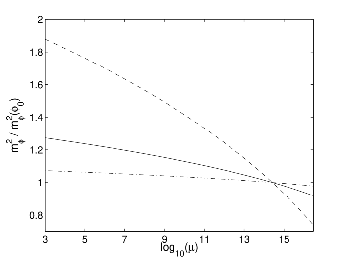
Figure 4: The running of $m^{2}_{\phi}$ for the $LLe$ inflaton when the saddle point is at $\phi_{0}=2.6\times 10^{14}$GeV (corresponding to $n=6$, $m_{\phi}=1$ TeV and $\lambda=1$). The three curves correspond to different values of the ratio of gaugino mass to flat direction mass at the GUT scale: $\xi=2$ (dashed), $\xi=1$ (solid) and $\xi=0.5$ (dash-dot).

Thus radiative corrections modify $\alpha$ and we need to finetune the potential to a few (but not all) orders in perturbation theory. However, although not completely disastrous, this can hardly be considered a satisfactory situation, and in the conclusions we speculate about possible remedies.

4.3 The inflaton and LHC

Let us recall that the constraint on the mass of the $n=6$ flat direction inflaton in Eq. (27) reads

$$m_{\phi}(\phi_{0})\simeq 100\,\rm{GeV}\,\cdot\lambda^{-1}\,\left(\frac{{\cal N}_{\rm COBE}}{50}\right)^{-4}\,.$$ (77)

As mentioned earlier, this is the bound on the mass of the flat direction during inflation, determined at the scale $\phi=\phi_{0}$. Since the inflaton mass runs from $\phi_{0}$ down to the LHC energy scales, it will also get scaled.

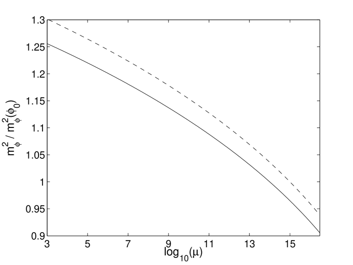
Figure 5: The same as Fig. 1 but with $\phi_{0}=10^{14}$GeV (solid) and $\phi_{0}=10^{15}$GeV (dashed), and $\xi=1$.

For ${\bf LLe}$ we see from the solution, Eq. (70), that the flat direction mass only gets larger due to the gaugino running,

$$m_{\phi}^{2}=m_{\phi}^{2}(\mu_{0})+{\tilde{m}_{2}}^{2}(\mu_{0})-{\tilde{m}_{2}}^{2}+\frac{1}{11}\left({\tilde{m}_{1}}^{2}(\mu_{0})-{\tilde{m}_{1}}^{2}\right)\,.$$ (78)

This has been depicted in Figs. 4 and 5. The $x$-axis is the scale $\mu$ which varies from the saddle point VEV at $\phi_{0}$ down to $1$ TeV scale, where LHC is probing new physics. We have also assumed unification of gauge couplings at the GUT scale. We find that the mass of the inflaton increases only very slightly at the TeV scale. In Fig. 4 we see that the increase is $\sqrt{1.9}\times 100,~{}\sqrt{1.3}\times 100,~{}\sqrt{1.1}\times 100$ GeV, for $\xi=2,1,0.5$, respectively. Changing the initial VEV from $10^{14}$ GeV to $10^{15}$ GeV results only in a minor modification in the running of $m^{2}_{\phi}$. This has been depicted in Fig. 5.

The mass at the TeV scale will increase further if $\lambda$ decreases much below one. For $\lambda=10^{-2}$, the bound exceeds $10$ TeV which escapes LHC limit. On the other hand, note that LHC will never probe the flat direction mass directly, but may set a limit on the slepton masses. However, we do not claim that LHC can discover MSSM inflation, but it can certainly rule out the possibility. If LHC does not find low energy supersymmetry within $\sim$ TeV, then MSSM inflation is effectively ruled out.

The situation would be similar for ${\bf udd}$ without the top squark. For the ${\bf u_{3}dd}$ direction it is possible that the inflaton mass gets even smaller at the weak scale.

4.4 $A_{6}$ vs. $A_{3}$

One final comment is in order before closing this Section. Unlike $m_{\phi}$, there is no prospect of measuring the $A$ term, because it is related to the non-renormalizable interactions which are suppressed by $M_{\rm P}$. However, a knowledge of supersymmetry breaking sector and its communication with the observable sector may help to link the non-renormalizable $A$-term under consideration to the renormalizable ones.

To elucidate this, let us consider the Polonyi model where a general $A$-term at a tree level is given by

$$m_{3/2}[(a-3)W+\phi(dW/d\phi)],$$

with $a=3-\sqrt{3}$ [24]. One then finds a relationship between $A$-terms corresponding to $n=6$ and $n=3$ superpotential terms, denoted by $A_{6}$ and $A_{3}$ respectively, at high scales:

$$A_{6}={3-\sqrt{3}\over 6-\sqrt{3}}A_{3}\,.$$ (79)

One can then use relevant RG equations to relate $A_{6}$ which is relevant for inflation, to $A_{3}$ at the weak scale, which can be constrained and/or measured. In principle this can also be done in general, provided that we have sufficient information about the supersymmetry breaking sector and its communication with the MSSM sector.

4.5 Supergravity corrections

SUGRA corrections often destroy the slow roll predictions of inflationary potentials; this is the notorious SUGRA-$\eta$ problem [27]. In general, the effective potential depends on the Kähler potential $K$ as $V\sim\left(e^{K(\varphi^{\ast},\varphi)/M_{\rm P}^{2}}V(\phi)\right)$ so that there is a generic SUGRA contribution to the flat direction potential of the type

$$V(\phi)=H^{2}M_{\rm P}^{2}f\left(\frac{\phi}{M_{\rm P}}\right)\,,$$ (80)

where $f$ is some function (typically a polynomial). Such a contribution usually gives rise to a Hubble induced correction to the mass of the flat direction with an unknown coefficient, which depends on the nature of the Kähler potential .

Let us compare the non-gravitational contribution, Eq. (2), to that of Hubble induced contribution, Eq. (80). Writing $f\sim\left(\phi/M_{\rm P}\right)^{p}$ where $p\geq 1$ is some power, we see that non-gravitational part dominates whenever

$$H_{\rm inf}^{2}M_{\rm P}^{2}\left(\frac{\phi}{M_{\rm P}}\right)^{p}\ll m_{\phi}^{2}\phi_{0}^{2}\,,$$ (81)

so that the SUGRA corrections are negligible as long as $\phi_{0}\ll M_{\rm P}$, as is the case here (note that $H_{\rm inf}M_{\rm P}\sim m_{\phi}\phi_{0}$). The absence of SUGRA corrections is a generic property of this model. Note also that although non-trivial Kähler potentials give rise to non-canonical kinetic terms of squarks and sleptons, it is a trivial exercise to show that at sufficiently low scales, $H_{\rm inf}\ll m_{\phi}$, and small VEVs, they can be rotated to a canonical form without affecting the potential .

5 End of MSSM inflation

5.1 Reheating and Thermalization

After the end of inflation, the flat direction starts rolling towards its global minimum. At this stage the dominant term in the scalar potential will be: $m_{\phi}\phi^{2}/2$. Since the frequency of oscillations is $\omega\sim m_{\phi}\sim 10^{3}H_{\rm inf}$, the flat direction oscillates a large number of times within the first Hubble time after the end of inflation. Hence the effect of expansion is negligible.

We recall that the curvature of the potential along the angular direction is much larger than $H^{2}_{\rm inf}$. Therefore, the flat direction has settled at one of the minima along the angular direction during inflation from which it cannot be displaced by quantum fluctuations. This implies that no torque will be exerted, and hence the flat direction motion will be one dimensional, i.e. along the radial direction.

Flat direction oscillations excite those MSSM degrees of freedom which are coupled to it. The inflaton, either ${\bf LLe}$ or ${\bf u}{\bf d}{\bf d}$ flat direction, is a linear combination of slepton or squark fields. Therefore inflaton has gauge couplings to the gauge/gaugino fields and Yukawa couplings to the Higgs/Higgsino fields. As we will see particles with a larger couplings are produced more copiously during inflaton oscillations. Therefore we focus on the production of gauge fields and gauginos. Keep in mind that the VEV of the MSSM flat direction breaks the gauge symmetry spontaneously, for instance ${\bf udd}$ breaks $SU(3)_{C}\times U(1)_{Y}$ while ${\bf LLe}$ breaks $SU(2)_{W}\times U(1)_{Y}$, therefore, induces a supersymmetry conserving mass $\sim g\langle\phi(t)\rangle$ to the gauge/gaugino fields in a similar way as the Higgs mechanism, where $g$ is a gauge coupling. When the flat direction goes to its minimum, $\langle\phi(t)\rangle=0$, the gauge symmetry is restored. In this respect the origin is a point of enhanced symmetry [6].

There can be various phases of particle creation in this model, here we briefly summarize them below. Let us elucidate the physics, by considering the case when ${\bf LLe}$ flat direction is the inflaton.

• Tachyonic preheating:
  Right after the end of inflation, when we are close to the saddle point, the second derivative is negative. One might suspect that this would trigger tachyonic instability in the inflaton fluctuations which will then excite the inflaton couplings to matter [31, 33].

  However the situation is different in our case. As mentioned, only inflaton fluctuations with a physical momentum $k\mathrel{\lower 4.0pt\vbox{\hbox{$<$}\hbox{$\sim$}}}m_{\phi}$ will have a tachyonic instability. Moreover $V^{\prime\prime}<0$ only at field values which are $\sim\phi_{0}$. Tachyonic effects are therefore expected be negligible since, unlike the case in [31], the homogeneous mode has a VEV which is hierarchically larger than $m_{\phi}$ (we remind that $\phi_{0}\geq 10^{14}$ GeV) and oscillates at a frequency $\omega\sim m_{\phi}$. Further note fields which are coupled to the inflaton acquire a very large mass $\sim h\phi_{0}$ from the homogeneous piece which suppresses non-perturbative production of their quanta at large inflaton VEVs. We conclude that tachyonic effects, although genuinely present, do not lead to significant particle production in our case.

• Instant preheating:
  An efficient bout of particle creation occurs when the inflaton crosses the origin, which happens twice in every oscillation. The reason is that fields which are coupled to the inflaton are massless near the point of enhanced symmetry. Mainly electroweak gauge fields and gauginos are then created as they have the largest coupling to the flat direction. The production takes place in a short interval, $\Delta t\sim\left(gm_{\phi}\phi_{0}\right)^{-1/2}$, where $\phi_{0}\sim 10^{14}$ GeV is the initial amplitude of the inflaton oscillation, during which quanta with a physical momentum $k\mathrel{\lower 4.0pt\vbox{\hbox{$<$}\hbox{$\sim$}}}\left(gm_{\phi}\phi_{0}\right)^{1/2}$ are produced. The number density of gauge/gaugino degrees of freedom is given by [34]

  $$n_{g}\approx{\left(gm_{\phi}\phi_{0}\right)^{3/2}\over 8\pi^{3}}\,.$$ (82)

  As the inflaton VEV is rolling back to its maximum value $\phi_{0}$, the mass of the produced quanta $g\langle\phi(t)\rangle$ increases. The gauge and gaugino fields can (perturbatively) decay to the fields which are not coupled to the inflaton, for instance to (s)quarks. Note that (s)quarks are not coupled to the flat direction, hence they remain massless throughout the oscillations. The total decay rate of the gauge/gaugino fields is then given by $\Gamma=C\left(g^{2}/48\pi\right)g\phi$, where $C\sim{\cal O}(10)$ is a numerical factor counting for the multiplicity of final states.

  The decay of the gauge/gauginos become efficient when

  $$\langle\phi\rangle\simeq\left({48\pi m_{\phi}\phi_{0}\over Cg^{3}}\right)^{1/2}\,.$$ (83)

  Here we have used $\langle\phi(t)\rangle\approx\phi_{0}m_{\phi}t$, which is valid when $m_{\phi}t\ll 1$, and $\Gamma\simeq t^{-1}$, where $t$ represents the time that has elapsed from the moment that the inflaton crossed the origin. Note that the decay is very quick compared with the frequency of inflaton oscillations, i.e. $\Gamma\gg m_{\phi}$. It produces relativistic (s)quarks with an energy:

  $$E=\frac{1}{2}g\phi(t)\simeq\left({48\pi m_{\phi}\phi_{0}\over Cg}\right)^{1/2}\,.$$ (84)

  The ratio of energy density in relativistic particles thus produced $\rho_{rel}$with respect to the total energy density $\rho_{0}$ follows from Eqs. (82), (84):

  $${\rho_{rel}\over\rho_{0}}\sim 10^{-2}g\,,$$ (85)

  where we have used $C\sim{\cal O}(10)$. This implies that a fraction $\sim{\cal O}(10^{-2})$ of the inflaton energy density is transferred into relativistic (s)quarks every time that the inflaton passes through the origin. This is so-called instant preheating mechanism [35] . It is quite an efficient mechanism in our model as it can convert almost all of the energy density in the inflaton into radiation within a Hubble time (note that $H^{-1}_{\rm inf}\sim 10^{3}m^{-1}_{\phi}$) .

5.2 Towards thermal equilibrium

A full thermal equilibrium is reached when ${\it a)~{}kinetic}$ and ${\it b)~{}chemical~{}equilibrium}$ are established. The maximum (hypothetical) temperature attained by the plasma would be given by:

$$T_{max}\sim V^{1/4}\sim\left(m_{\phi}\phi_{0}\right)^{1/2}\geq 10^{9}~{}{\rm GeV}\,.$$ (86)

This temperature may be too high and could lead to thermal overproduction of gravitinos [37, 38]. However the dominant source of gravitino production in a thermal bath is scattering which include an on-shell gluon or gluino leg. In the next subsection we describe a natural solution to this problem and show that the final reheat temperature is actually well below Eq. (86), i.e. $T_{R}\ll T_{max}$.

One comment is in order before closing this subsection. The gravitinos can also be created non-perturbatively during inflaton oscillations, both of the helicity $\pm 3/2$ [39] and helicity $\pm 1/2$ states [40]. In models of high scale inflation (i.e. $H_{\rm inf}\gg m_{3/2}$) helicity $\pm 1/2$ states can be produced very efficiently (and much more copiously than helicity $\pm 3/2$ states). At the time of production these states mainly consist of the inflatino (inflaton’s superpartner). However these fermions also decay in the form of inflatino, which is coupled to matter with a strength which is equal to that of the inflaton. Therefore, they inevitably decay at a similar rate as that of inflaton, and hence pose no threat to primordial nucleosynthesis [41].

In the present case $m_{\phi}\sim m_{3/2}\gg H_{\rm inf}$. Therefore low energy supersymmetry breaking is dominant during inflation, and hence helicity $\pm 1/2$ states of the gravitino are not related to the inflatino (which is a linear combination of leptons or quarks)at any moment of time. As a result helicity $\pm 1/2$ and $\pm 3/2$ states are excited equally, and their abundances are suppressed due to kinematical phase factor. Moreover there will be no dangerous gravitino production from perturbative decay of the inflaton quanta [42, 43]. The reason is that the inflaton is not a gauge singlet and has gauge strength couplings to other MSSM fields. This makes the $inflaton\rightarrow inflatino~{}+~{}gravitino$  decay mode totally irrelevant.

5.3 Solution to the gravitino problem

In order to suppress thermal gravitino production it is sufficient to make gluon and gluino fields heavy enough such that they are not kinematically accessible to the reheated plasma, even if other degrees of freedom reach full equilibrium (for a detailed discussion on thermalization in supersymmetric models and its implications, see [5, 6]). This suggests a natural solution to the thermal gravitino problem in the case of our model. Consider another flat direction with a non-zero VEV, denoted by $\varphi$, which spontaneously breaks the $SU(3)_{C}$ group. For example, if ${\bf LLe}$ is the inflaton, then ${\bf udd}$ provides a unique candidate which can simultaneously develop VEV The induced mass for gluon/gluino fields will be:

$$m_{G}\sim g\langle\varphi(t)\rangle<g\phi_{0}\,.$$ (87)

The inequality arises due to the fact that the VEV of $\varphi$ cannot exceed that of the inflaton $\phi$ since its energy density should be subdominant to the inflaton energy density.

If $g\varphi_{0}\gg T_{max}$ the gluon/gluino fields will be too heavy and not kinematically accessible to the reheated plasma. Here $\varphi_{0}$ is the VEV of ${\bf udd}$ at the beginning of inflaton oscillations. In a radiation-dominated Universe the Hubble expansion redshifts the flat direction VEV as $\langle\varphi\rangle\propto H^{3/4}$, which is a faster rate than the change in the temperature $T\propto H^{1/2}$. Once $g\langle\varphi\rangle\simeq T$, gluon/gluino fields come into equilibrium with the thermal bath. As pointed out in Refs. [5, 6], if the initial VEV of ${\bf udd}$ is

$$\varphi_{0}>10^{10}~{}{\rm GeV}\,,$$ (88)

then the temperature at which gluon/gluino become kinematically accessible, i.e. $g\langle\varphi\rangle\simeq T$, is given by  [6] :

$$T_{\rm R}\leq 10^{7}~{}{\rm GeV}\,.$$ (89)

This is the final reheat temperature at which gluons and gluinos are all in thermal equilibrium with the other degrees of freedom. The standard calculation of thermal gravitino production via scatterings can then be used for $T\leq T_{\rm R}$. Note however that $T_{\rm R}$ is sufficiently low to avoid thermal overproduction of gravitinos.

Finally, we also make a comment on the cosmological moduli problem. The moduli are generically displaced from their true minimum if their mass is less than the expansion rate during inflation. The moduli obtain a mass $\sim{\cal O}({\rm TeV})$ from supersymmetry breaking. They start oscillating with a large amplitude, possibly as big as $M_{\rm P}$, when the Hubble parameter drops below their mass. Since moduli are only gravitationally coupled to other fields, their oscillations dominate the Universe while they decay very late. The resulting reheat temperature is below MeV, and is too low to yield a successful primordial nucleosynthesis.

However, in our case $H_{\rm inf}\ll{\rm TeV}$ . This implies that quantum fluctuations cannot displace the moduli from their true minima during the inflationary epoch driven by MSSM flat directions. Moreover, any oscillations of the moduli will be exponentially damped during the inflationary epoch. Therefore our model is free from the infamous moduli problem.

6 Conclusion

The existence of a saddle point in the scalar potential of the ${\bf udd}$ or ${\bf LLe}$ MSSM flat directions appears, perhaps surprisingly, to provide all the necessary ingredients for an observationally realistic model of inflation [1]. MSSM inflation takes place at a low energy scale so that it is naturally free of supergravity and super-Planckian effects. The exceptional feature of the model, which sets it apart from conventional singlet field inflation models, is the fact that here the inflaton is a gauge invariant combination of the squark or slepton fields. As a consequence, the couplings of the inflaton to the MSSM matter and gauge fields are known. This makes it possible to address the questions of reheating and gravitino production in an unambiguous way, as we did in Sect. 5. Since ${\bf udd}$ and ${\bf LLe}$ are independently flat, therefore, if ${\bf LLe}$ is the inflaton, the ${\bf udd}$ direction can also acquire a large VEV simultaneously. This gives a large mass to gluons/gluinos which decouples them from the thermal bath, and hence suppresses thermal gravitino production. As discussed in Sect. 5, non-thermal production of gravitinos is negligible in our model.

In the MSSM inflation model the mass of the inflaton is not a free parameter but is related to the masses of e.g. sleptons, should the ${\bf LLe}$ direction be the inflaton. We have solved the appropriate RG equation equations to relate the inflaton mass to the slepton masses at energies accessible to accelerators such as LHC and found that LHC can indeed put a constraint on the model: it may not be able to verify it, but it certainly can rule it out.

The model predictions are not modified by supergravity corrections, i.e. the observables are insensitive to the nature of Kähler potential. MSSM inflation also illustrates that it is free from any Trans-Planckian corrections. MSSM inflation retains the successes of thermal production of LSP as a dark matter and the electroweak baryogenesis within MSSM.

The existence of the saddle point requires a fine-tuning of ratio of the soft breaking terms $A$ and $m$, or the parameter $\alpha$, as discussed in length in Sects. 3 and 4. We dealt both with the case of a local minimum and the case of $V^{\prime}(\phi)>0$. We found that a fine-tuning of the order of $10^{-9}$ is sufficient. It is therefore necessary to adjust the ratio $A/m$ up to few orders in perturbation theory. However, we find that the existence of the saddle point is not sensitive to radiative corrections so that saddle point inflation can always be achieved for some value of the ratio $A/m$.

However, it is conceivable that the mechanism of supersymmetry breaking, which lies outside the effective theory of MSSM combined with gravity discussed in this paper, could remove the fine-tuning in some natural, dynamical way. For instance, $A/m$ could turn out to be a renormalization group fixed point so that once the ratio is fixed, it would remain fixed at all orders (for example, see [44]). This requires a detailed investigation, but it is warranted by the simplicity and the apparent success of MSSM flat direction inflation, which is unique in being both a successful model of inflation and at the same time having a concrete and real connection to physics that can be observed in earth bound laboratories.

7 Acknowledgments

We wish to thank Cliff Burgess, Manuel Drees, John Ellis, Jaume Garriga, Alex Kusenko, and Tony Riotto for valuable discussions and various suggestions they have made. We also benefitted from the discussions with Shanta de Alwis, Steve Abel, Mar Bastero-Gil, Micha Berkhooz, Zurab Berezhiani, Robert Brandenberger, Ramy Brustein, Damien Easson, Gordy Kane, Justin Khoury, George Lazarides, Andrei Linde, Andrew Liddle, Hans Peter Nilles, Pavel Naselsky, Maxim Pospelov, Subir Sarkar, Qaisar Shafi, Misha Shaposhnikov, Scott Thomas and Igor Tkachev. We would also like to thank the Galileo Galilei Institute for Theoretical Physics for the hospitality and the INFN for partial support during the completion of this work. The research of RA was supported by Perimeter Institute for Theoretical Physics. Research at Perimeter Institute is supported in part by the Government of Canada through NSERC and by the province of Ontario through MEDT. KE is supported by the Academy of Finland grant 108712. The research of KE, AJ, JGB and AM are partly supported by the European Union through Marie Curie Research and Training Network “UNIVERSENET” (MRTN-CT-2006-035863).

References

- [1] R. Allahverdi, K. Enqvist, J. Garcia-Bellido and A. Mazumdar, “Gauge invariant MSSM inflaton,” Phys. Rev. Lett. 97, 191304 (2006) [hep-ph/0605035].
- [2] K. Enqvist and A. Mazumdar, Phys. Rept. 380, 99 (2003) [hep-ph/0209244]. M. Dine and A. Kusenko, Rev. Mod. Phys. 76, 1 (2004) [hep-ph/0303065].
- [3] R. Allahverdi, A. Kusenko and A. Mazumdar, arXiv:hep-ph/0608138.
- [4] D. H. Lyth and A. Riotto, Phys. Rept. 314, 1 (1999) [hep-ph/9807278].
- [5] R. Allahverdi and A. Mazumdar, “Towards a successful reheating within supersymmetry,” arXiv:hep-ph/0603244.
- [6] R. Allahverdi and A. Mazumdar, JCAP 0610, 008 (2006) [hep-ph/0512227].
- [7] R. Allahverdi and A. Mazumdar, “Quasi-thermal universe and its implications for gravitino production, baryogenesis and dark matter,” arXiv:hep-ph/0505050.
- [8] R. Allahverdi and A. Mazumdar, “Longevity of supersymmetric flat directions,” arXiv:hep-ph/0608296.
- [9] J. C. B. Sanchez, K. Dimopoulos and D. H. Lyth, JCAP 0701, 015 (2007) [hep-ph/0608299].
- [10] D. H. Lyth, arXiv:hep-ph/0605283.
- [11] T. Gherghetta, C. F. Kolda and S. P. Martin, Nucl. Phys. B 468, 37 (1996) [hep-ph/9510370].
- [12] M. Dine, L. Randall and S. Thomas, Phys. Rev. Lett. 75, 398 (1995) [hep-ph/9503303]; Nucl. Phys. B 458, 291 (1996) [hep-ph/9507453].
- [13] R. Allahverdi, K. Enqvist, A. Jokinen and A. Mazumdar, “Identifying the curvaton within MSSM,” JCAP 0610, 007 (2006) [hep-ph/0603255].
- [14] A. H. Guth, Phys. Rev. D 23, 347 (1981).
- [15] A. Jokinen and A. Mazumdar, Phys. Lett. B 597, 222 (2004) [hep-th/0406074].
- [16] G. F. Giudice and R. Rattazzi, Phys. Rept. 322, 419 (1999) [hep-ph/9801271].
- [17] N. Arkani-Hamed, S. Dimopoulos, G. F. Giudice and A. Romanino, Nucl. Phys. B 709, 3 (2005) [hep-ph/0409232].
- [18] R. Allahverdi, A. Jokinen, and A. Mazumdar, “Sub-eV Hubble scale inflation within GMSB”, [hep-ph/0610243].
- [19] K. Enqvist, A. Jokinen and A. Mazumdar, JCAP 0401, 008 (2004) [hep-ph/0311336].
- [20] C. P. Burgess, R. Easther, A. Mazumdar, D. F. Mota and T. Multamaki, JHEP 0505, 067 (2005) [hep-th/0501125].
- [21] R. Allahverdi and A. Mazumdar, “Spectral tilt in A-term inflation,” arXiv:hep-ph/0610069.
- [22] D.N. Spergel, et.al., astro-ph/0603449.
- [23] R. Coleman and F. De Luccia, Phys. Rev. D 21, 3305 (1980).
- [24] H. P. Nilles, Phys. Rept. 110, 1 (1984).
- [25] Y. Yamada, Phys. Rev. D 50, 3537 (1995) [hep-ph/9401241].
- [26] K. Enqvist, A. Jokinen and J. McDonald, Phys. Lett. B 483, 191 (2000) [hep-ph/0004050].
- [27] M. Dine, W. Fischler, and D. Nemeschansky, Phys. Lett. B 136, 169 (1984); G. D. Coughlan, R. Holman, P. Ramond, and G. G. Ross, Phys. Lett. B 140, 44 (1984); A. S. Goncharov, A. D. Linde, and M. I. Vysotsky, Phys. Lett. B 147, 279 (1984); O. Bertolami, and G. G. Ross, Phys. Lett. B 183, 163 (1987); E. J. Copeland, A. R. Liddle, D. H. Lyth, E. D. Stewart, and D. Wands, Phys. Rev. D 49, 6410 (1994).
- [28] M. K. Gaillard, H. Murayama and K. A. Olive, Phys. Lett. B 355, 71 (1995) [hep-ph/9504307].
- [29] R. Allahverdi, M. Drees and A. Mazumdar, Phys. Rev. D 65, 065010 (2002) [hep-ph/0108225].
- [30] See for instance, C. P. Burgess, J. Cline and R. Holman, JCAP 0310, 004 (2003) [hep-th/0306079].
- [31] G. N. Felder, J. Garcia-Bellido, P. B. Greene, L. Kofman, A. D. Linde and I. Tkachev, Phys. Rev. Lett. 87, 011601 (2001) [hep-ph/0012142].
- [32] R. Allahverdi, R. H. A. Shaw and B. A. Campbell, Phys. Lett. B 473, 246 (2000) [hep-ph/9909256]; M. Postma and A. Mazumdar, JCAP 0401, 005 (2004) [hep-ph/0304246].
- [33] J. Garcia-Bellido and E. Ruiz Morales, Phys. Lett. B 536, 193 (2002) [hep-ph/0109230].
- [34] L. Kofman, A. D. Linde and A. A. Starobinsky, Phys. Rev. Lett. 73, 3195 (1994) [hep-th/9405187]; L. Kofman, A. D. Linde and A. A. Starobinsky, Phys. Rev. D 56, 3258 (1997) [hep-ph/9704452].
- [35] G. N. Felder, L. Kofman and A. D. Linde, Phys. Rev. D 59, 123523 (1999) [hep-ph/9812289].
- [36] R. Allahverdi, R. Brandenberger and A. Mazumdar, Phys. Rev. D 70, 083535 (2004) [hep-ph/0407230].
- [37] J. R. Ellis, J. E. Kim and D. V. Nanopoulos, Phys. Lett. B 145, 181 (1984).
- [38] M. Bolz, A. Brandenburg and W. Buchmüller, Nucl. Phys. B 606, 518 (2001) [hep-ph/0012052].
- [39] A. L. Maroto and A. Mazumdar, Phys. Rev. Lett. 84, 1655 (2000) [hep-ph/9904206].
- [40] R. Kallosh, L. Kofman, A. D. Linde and A. Van Proeyen, Phys. Rev. D 61, 103503 (2000) [hep-th/9907124].
- [41] R. Allahverdi, M. Bastero-Gil and A. Mazumdar, Phys. Rev. D 64, 023516 (2001) [hep-ph/0012057]. H. P. Nilles, M. Peloso and L. Sorbo, Phys. Rev. Lett. 87, 051302 (2001) [hep-ph/0102264]. H. P. Nilles, M. Peloso and L. Sorbo, JHEP 0104, 004 (2001) [hep-th/0103202].
- [42] R. Allahverdi, K. Enqvist and A. Mazumdar, Phys. Rev. D 65, 103519 (2002) [hep-ph/0111299].
- [43] K. Enqvist, S. Kasuya and A. Mazumdar, Phys. Rev. Lett. 89, 091301 (2002) [hep-ph/0204270]. K. Enqvist, S. Kasuya and A. Mazumdar, Phys. Rev. D 66, 043505 (2002) [hep-ph/0206272].
- [44] M. Lanzagorta and G. G. Ross, Phys. Lett. B 349, 319 (1995) [hep-ph/9501394]. M. Lanzagorta and G. G. Ross, Phys. Lett. B 364, 163 (1995) [hep-ph/9507366].