CERN-PH-TH/2006-207
NUB-TH-3259
v1 Oct 11 2006

Abstract

We investigate a new type of dark matter with couplings to ordinary matter naturally suppressed by at least 1 order of magnitude compared to weak interactions. Despite the extra-weak interactions massive particles of this type (XWIMPs) can satisfy the Wilkinson Microwave Anisotropy Probe (WMAP) relic density constraints due to coannihilation if their masses are close to that of the lightest state of the minimal supersymmetric standard model (MSSM). The region in the parameter space of a suitably extended minimal supergravity (mSUGRA) model consistent with the WMAP3 constraints on XWIMPs is determined. Plots for sparticles’ masses are given which can be subject to test at the Large Hadron Collider. As an example for an explicit model we show that such a form of dark matter can arise in certain $Z^{\prime}$ extensions of the MSSM. Specifically we consider an Abelian extension with spontaneous gauge symmetry breaking via Fayet-Iliopoulos D-terms in the hidden sector. The LSP of the full model arises from the extra $U(1)_{X}$ sector with extra-weak couplings to Standard Model particles due to experimental constraints. With R-parity conservation the new XWIMP is a candidate for cold dark matter. In a certain limit the model reduces to the Stueckelberg extension of the MSSM without a Higgs mechanism, and wider ranges of models with similar characteristics are easy to construct.

1 Introduction

The nature of dark matter [1] and dark energy continues to be one of the primary open questions in both particle theory and cosmology. It is now widely believed that dark matter must be constituted of particles outside the standard list of known particles. Chief among these are the so called weakly interacting massive particles (WIMPS). Supersymmetry with R-parity conservation leads naturally to such a particle in the form of the lightest supersymmetric particle (LSP). In the framework of SUGRA unified models the lightest neutralino is a particularly attractive possibility.

In this paper we investigate a new possibility in supersymmetric models, where the dark matter candidate has extra-weak interactions with matter; interactions weaker than weak interactions by at least one order of magnitude. We refer to these particles as XWIMPs. We will show that such a possibility can occur naturally in certain extensions of the minimal supersymmetric Standard Model (MSSM) by Abelian gauge symmetries $U(1)_{X}$. One such class has been analyzed recently [2, 3, 4, 5, 6, 7]. Models of this type are based on the Stueckelberg mechanism which arises quite naturally in string and D brane models. Further, some of the specific features of the models of [2, 3, 4, 5, 6, 7] and of the type discussed here may have a string realization[8]. A more detailed discussion of the motivation for such models may be found in the above references. But there may be a wider range of models where extra-weak dark matter can appear. The relic density analysis of XWIMPS requires careful study which will be discussed later in this paper.

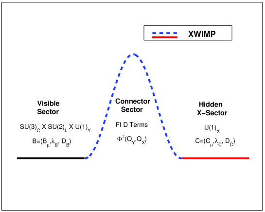
Figure 1: The generation of the extra-weakly interacting massive particles. An XWIMP is a linear combination of fields in the hidden sector and in the connector sector, and its interactions with the MSSM particles are suppressed.

The basic elements of the models we discuss are exhibited in Fig.(1) and involve three sectors: $(i)$ a visible sector where the fields of the SM or the MSSM reside, $(ii)$ a hidden sector which is neutral under the SM gauge group, and $(iii)$ a third sector [9] which is non-trivial under the SM and the hidden sector gauge symmetry. Aside from gravity, the fields of the visible sector and the hidden sector communicate only via this third sector which we therefore call the “connector sector”. Interactions with hidden particles can of course modify predictions of the SM and are thus highly constrained by the precision data from LEP and Tevatron, see e.g. [6].

In the following, we construct explicit simple models where the gauge group in the hidden sector is just an Abelian $U(1)_{X}$ with spontaneous breaking and a massive $Z^{\prime}$ gauge boson. Such Abelian extensions of the MSSM occur in a wide class of models including grand unified models, string and brane models [10, 11, 12, 8, 13, 14, 15]. The explicit elements of our first example are as follows:

1. The visible sector contains gauge, matter and Higgs superfields of the MSSM charged under the gauge group $SU(3)_{C}\times SU(2)_{L}\times U(1)_{Y}$, but neutral under $U(1)_{X}$.

2. The hidden sector contains the gauge superfield for $U(1)_{X}$ which are neutral under the Standard Model gauge group.

3. The connector sector contains the chiral fields $\phi^{\pm}$ with charges $\pm Q_{X}$ under $U(1)_{X}$ and $\pm Y_{\phi}$ under $U(1)_{Y}$. They thus carry dual quantum numbers. The fields in the visible and in the hidden sectors can communicate only via couplings with these connector fields.

Spontaneous breaking of the $U(1)_{X}$ generates a mixing between the hidden and the visible fields. We will implement this breaking via Fayet-Illiopoulos D-terms [16]. The parameters that measure the mixing are highly suppressed because of the precision constraints on the electroweak predictions. Their smallness is responsible for the extra-weak interactions of the hidden and the connector fields with the fields in the MSSM.

If the LSP of the $U(1)_{X}$ sector which we call the XLSP is lighter than the LSP of the visible sector, it will be the LSP of the whole system. With R-parity conservation, it is then an XWIMP candidate for cold dark matter.

We will also show that the above class of models reduces in a certain limit to the Stueckelberg extension of MSSM introduced in [3]. It is also interesting to investigate if an XWIMP can arise in models where mixing between the visible and the hidden sector occurs in the gauge kinetic energy [18]. In a supersymmetrization of such a model with off-diagonal kinetic terms one as well finds a mixing between the neutral fermions: i.e., the gauginos and the chiral fermions of the visible and the hidden sector. Thus, these models provide another class with potential of an XWIMP responsible for dark matter. More generally, there may be a much wider range of models with similar properties.

The outline of the rest of the paper is as follows: In Sec.2 we work out a $U(1)_{X}$ extension of the MSSM with symmetry breaking via Fayet-Illiopoulos D-terms [16] mixing between the $U(1)_{X}$ and the $U(1)_{Y}$ fields. The neutralino sector of this system has a $6\times 6$ mass matrix. It can lead to an LSP with extra-weak interactions composed mostly of neutral fermions in the hidden sector. The model reduces in a certain limit to the Stueckelberg extension of MSSM (the StMSSM) [3]. We briefly discuss the electroweak constraints on the parameters of the model. As an alternative we next consider a mixing between the visible and hidden sectors originating from the gauge kinetic energy which works very similarly. In Sec. 3 we analyze the relic density of XWIMPs and show that it is possible to satisfy the experimental constraints via the process of coannihilation. A detailed numerical analysis shows that XWIMPs are candidates for cold dark matter consistent with the recent WMAP data. The sensitivity of the analysis on the errors in the top quark mass under the constraints of radiative breaking of the electroweak symmetry is also discussed. Conclusions are given in Sec. 4.

2 Extra-weak dark matter in $Z^{\prime}$ models

To start with, we introduce a class of extensions of the MSSM where a natural mixing of the neutral MSSM fields with fields from the hidden sector appears via off-diagonal mass matrices. Towards the end of this section we also discuss other possibilities to facilitate a mixing of a very similar type.

2.1 Broken $U(1)_{X}$ with Fayet-Iliopoulos terms

A $U(1)_{X}$ extension of the MSSM with a Fayet-Iliopoulos (FI) D-term can lead in a natural manner to extra-weakly interacting dark matter constrained by LEP and Tevatron data. Specific $U(1)$ extensions have been studied quite extensively in the literature [13, 10, 19]. The features of our model were already explained in the introduction. The full gauge symmetry of the model is $SU(3)_{C}\times SU(2)_{L}\times U(1)_{Y}\times U(1)_{X}$. It differs from previous formulations in that a FI D-term breaks the extra $U(1)$ gauge symmetry instead of an F-term. The Abelian vector fields consist of the $U(1)_{Y}$ vector multiplet $(B_{\mu},\lambda_{B},D_{B})$ and the $U(1)_{X}$ vector multiplet $(C_{\mu},\lambda_{C},D_{C})$ with gauge kinetic Lagrangian given by

$${\cal L}_{\rm gkin}=-\frac{1}{4}B_{\mu\nu}B^{\mu\nu}-i\lambda_{B}\sigma^{\mu}\partial_{\mu}\bar{\lambda}_{B}+\frac{1}{2}D_{B}^{2}-\frac{1}{4}C_{\mu\nu}C^{\mu\nu}-i\lambda_{C}\sigma^{\mu}\partial_{\mu}\bar{\lambda}_{C}+\frac{1}{2}D_{C}^{2}\ .$$ (1)

The superfields $\Phi^{\pm}$ with components $(\phi^{\pm},f^{\pm},F^{\pm})$ are described by

$${\cal L}_{\Phi} = -|D_{\mu}\phi^{+}|^{2}-if^{+}\sigma^{\mu}D_{\mu}\bar{f}^{+}-\sqrt{2}\left(ig_{X}Q_{X}\phi^{+}\bar{f}^{+}\bar{\lambda}_{C}+ig_{Y}Y_{\phi}\phi^{+}\bar{f}^{+}\bar{\lambda}_{B}+\,{\rm h.c.}\,\right)$$ (2)

$$+g_{X}D_{C}(\bar{\phi}^{+}Q_{X}\phi^{+})+g_{Y}D_{B}(\bar{\phi}^{+}Y_{\phi}\phi^{+})+\{\Phi^{+}\rightarrow\Phi^{-}\}\ ,$$

where $F^{\pm}$ is set to zero and the covariant derivatives of the scalars are

$$D_{\mu}\phi^{\pm}=(\partial_{\mu}\pm ig_{X}Q_{X}C_{\mu}\pm ig_{Y}Y_{\phi}B_{\mu})\phi^{\pm}\ .$$ (3)

Next we add to the mix the FI terms

$${\cal L}_{\rm FI}=\xi_{X}D_{C}+\xi_{Y}D_{B}\ .$$ (4)

Elimination of the D terms gives us the scalar potential

$$V=\frac{g_{X}^{2}}{2}\Big{(}Q_{X}|\phi^{+}|^{2}-Q_{X}|\phi^{-}|^{2}+\xi_{X}\Big{)}^{2}+\frac{g_{Y}^{2}}{2}\Big{(}Y_{\phi}|\phi^{+}|^{2}-Y_{\phi}|\phi^{-}|^{2}+\xi_{Y}\Big{)}^{2}\ .$$ (5)

Minimization of the potential leads to

$$\langle\phi^{+}\rangle=0\ ,\quad\langle\phi^{-}\rangle=\sqrt{\frac{g_{X}^{2}\xi_{X}Q_{X}+g_{Y}^{2}\xi_{Y}Y_{\phi}}{g_{X}^{2}Q_{X}^{2}+g_{Y}^{2}Y_{\phi}^{2}}}\ .$$ (6)

We consider the bosonic sector first. Spontaneous breaking of the electroweak symmetry gives rise to the mixing of the neutral gauge fields $(C^{\mu},B^{\mu},A^{3\mu})$, with $A^{\mu a}$ $(a=1,2,3)$ for the $SU(2)_{L}$ gauge fields. In this basis the mass matrix in the neutral sector is of the form

$$\left[\begin{array}[]{ccc}M_{1}^{2}&M_{1}M_{2}&0\\ M_{1}M_{2}&M_{2}^{2}+\frac{1}{4}v^{2}g_{Y}^{2}&-\frac{1}{4}v^{2}g_{2}g_{Y}\\ 0&-\frac{1}{4}v^{2}g_{2}g_{Y}&\frac{1}{4}v^{2}g_{2}^{2}\end{array}\right]\ .$$ (7)

The parameters $M_{1}$, $M_{2}$ are defined so that

$$M_{1}=\sqrt{2}g_{X}Q_{X}\langle\phi^{-}\rangle\ ,\quad M_{2}=\sqrt{2}g_{Y}Y_{\phi}\langle\phi^{-}\rangle\ .$$ (8)

There is a single massless mode, the photon, and two massive modes the $Z$ and $Z^{\prime}$. Since $\langle\phi^{+}\rangle=0$, the superfield $\Phi^{+}$ does not enter in the mixings in the mass matrix for the fields in the hidden sector and the fields in the visible sector, and we do not consider it further. The CP-even component of the complex scalar $\phi^{-}$ mixes with the two CP-even Higgs fields of MSSM producing a $3\times 3$ mass matrix similar to the analysis given in Ref. [3, 4].

In the neutral fermionic sector there are two additional mass eigenstates beyond the four neutral fermionic states in the MSSM, $\lambda_{Y},\lambda_{3},\tilde{h}_{1},\tilde{h}_{2}$. One can reorganize the Weyl spinors in terms of four-component Majorana spinors $\chi_{S}$ (out of $f^{-}$) and $\lambda_{X}$ (out of $\lambda_{C}$) in a standard way. The $6\times 6$ neutralino mass matrix in the basis $((\chi_{S},\lambda_{X});(\lambda_{Y},\lambda_{3},\tilde{h}_{1},\tilde{h}_{2}))$ reads

$$\left[\matrix{0&M_{1}&M_{2}&0&0&0\cr M_{1}&\tilde{m}_{X}&0&0&0&0\cr M_{2}&0&\tilde{m}_{1}&0&-c_{\beta}s_{W}M_{0}&s_{\beta}s_{W}M_{0}\cr 0&0&0&\tilde{m}_{2}&c_{\beta}c_{W}M_{0}&-s_{\beta}c_{W}M_{0}\cr 0&0&-c_{\beta}s_{W}M_{0}&c_{\beta}c_{W}M_{0}&0&-\mu\cr 0&0&s_{\beta}s_{W}M_{0}&-s_{\beta}c_{W}M_{0}&-\mu&0}\right]\ .$$ (9)

A few explanations are in order: $\tilde{m}_{X}$ arises from the soft mass term $-\frac{1}{2}\tilde{m}_{X}\bar{\lambda}_{X}\lambda_{X}$, $M_{0}$ is the $Z$ boson mass at the tree level, $c_{W}=\cos\theta_{W}$, $s_{W}=\sin\theta_{W}$ with $\theta_{W}$ the weak angle, similarly $c_{\beta}=\cos\beta$, $s_{\beta}=\sin\beta$, with $\tan\beta=\langle H_{2}\rangle/\langle H_{1}\rangle$, and finally $\mu$ the Higgs mixing parameter of the MSSM. The mass eigenstates of the system are defined as the following six Majorana states

$$((\xi_{1}^{0},\xi_{2}^{0});(\chi_{1}^{0},\chi_{2}^{0},\chi_{3}^{0},\chi_{4}^{0}))\ ,$$ (10)

where $\chi_{a}^{0}$ $(a=1,2,3,4)$ are essentially the four neutralino states of the MSSM and the $\xi_{\alpha}^{0}$, $(\alpha=1,2)$ the two additional states composed mostly of the new neutral fermions.

We will discuss in a moment that the current electroweak data puts a stringent bound on $\epsilon=M_{2}/M_{1}$ such that $|\epsilon|\ll 1$ [6]. In this limit the masses of $\xi_{1}^{0},\xi_{2}^{0}$ are

$$m_{\xi_{1}^{0}}\simeq\sqrt{M_{1}^{2}+\frac{1}{4}\tilde{m}_{X}^{2}}-\frac{1}{2}\tilde{m}_{X},~{}~{}m_{\xi_{2}^{0}}\simeq\sqrt{M_{1}^{2}+\frac{1}{4}\tilde{m}_{X}^{2}}+\frac{1}{2}\tilde{m}_{X}\ .$$ (11)

For the case when the lightest of the MSSM neutralinos $\chi^{0}\equiv\chi_{1}^{0}$ is also lighter than $\xi^{0}\equiv\xi_{1}^{0}$ nothing much changes compared to the pure MSSM. The LSP of the MSSM will still be the LSP of the full system, and the dark matter candidate will be essentially the same as in the MSSM with minor modifications. However, a very different scenario emerges if $\xi^{0}$ is lighter than $\chi^{0}$ and becomes the LSP. The upper bound on $\epsilon$ translates to a suppression of the couplings of $\xi^{0}$ to MSSM fields relative to the couplings of $\chi^{0}$ by a factor of $\epsilon$. Roughly speaking one can treat $\xi^{0}$ as a standard LSP $\chi^{0}$ but with couplings appropriately suppressed by at least an order of magnitude. This is why we call $\xi^{0}$ extra-weakly interacting, an XWIMP.

2.2 Stueckelberg reduction of $U(1)_{X}$ extension

In a certain limit the model of the previous subsection reduces to the Stueckelberg extension of MSSM proposed in [3, 4]. To achieve the reduction we assume as is conventional in the analysis of MSSM that $\xi_{Y}$ is negligible. We consider now the limit $\langle\phi^{-}\rangle\rightarrow\infty$, $g_{X}Q_{X}\rightarrow 0$, and $g_{Y}Y_{\phi}\rightarrow 0$, with $M_{1}$ and $M_{2}$ fixed. This leads to

$$\frac{1}{2}|D_{\mu}\phi^{-}|^{2}=\frac{1}{2}(M_{1}C_{\mu}+M_{2}B_{\mu}+\partial_{\mu}a)^{2}+\frac{1}{2}(\partial_{\mu}\rho)^{2}\ .$$ (12)

where $\phi^{-}=\rho+ia$. The Lagrangian can be written $\mathcal{L}_{\Phi}=\mathcal{L}_{St}+\mathcal{L}_{\Phi^{+}}$ , where $\Phi^{+}$ is now completely decoupled from the vector multiplet and ${\cal L}_{\rm St}$ can be written

$${\cal L}_{\rm St} = -\frac{1}{2}(M_{1}C_{\mu}+M_{2}B_{\mu}+\partial_{\mu}a)^{2}-\frac{1}{2}(\partial_{\mu}\rho)^{2}-i\chi\sigma^{\mu}\partial_{\mu}\bar{\chi}$$

$$+\rho(M_{1}D_{C}+M_{2}D_{B})+\big{[}\chi(M_{1}\lambda_{C}+M_{2}\lambda_{B})+{\rm h.c.}\big{]}\ .$$

This arises from the following density in superfield notation

$${\cal L}_{\rm St}=\int d^{2}\theta d^{2}\bar{\theta}\ (M_{1}C+M_{2}B+S+\bar{S})^{2}\ ,$$ (14)

where $C$ and $B$ are gauge supermultiplets and $S$ a chiral supermultiplet. See [3, 4] for more details. With the above one then has exactly the Stueckelberg extension of the MSSM.

2.3 Electroweak constraints on mixing parameters

The $U(1)_{X}$ extension of MSSM of the type discussed in Secs.(2.1) and (2.2) has two mass parameters, $M_{1}$ and $M_{2}$, which can affect electroweak physics. However, since the Standard Model is already in excellent agreement with LEP and Tevatron data the above extensions are severely constrained. New physics can only be accommodated within the corridor of error bars consistent with precision measurements. For example, the SM prediction relating the $W$ and $Z$ masses (in the on-shell scheme) is given by [21]

$$\frac{M_{W}^{2}}{M_{Z}^{2}}+\frac{\pi\alpha}{\sqrt{2}G_{F}M_{W}^{2}(1-\Delta r)}=1\ .$$ (15)

In the above $\alpha$ is the fine structure constant at the scale $Q^{2}=0$, $G_{F}$ the Fermi constant, $\Delta r$ the radiative correction such that $\Delta r=0.0363\pm 0.0019$ [22], where the error in $\Delta r$ comes from the error in the top quark mass and in $\alpha(M^{2}_{Z})$. Using the current value of the $W$ mass $M_{W}=(80.425\pm 0.034)$ GeV [22] one finds the central value of $M_{Z}$ in excellent agreement with the current data, $M_{Z}=(91.1876\pm 0.0021)$ GeV. But the error of theoretical prediction is $\delta M_{Z}\sim 30$ MeV. Using techniques similar to the ones used in constraining extra dimensions [23] one may equate this error corridor in $M_{Z}$ to the shift in $M_{Z}$ due to its coupling to the Stueckelberg sector of the extended model. This constrains $\epsilon=M_{2}/M_{1}$ to lie in the range [6]

$$|\epsilon|\lesssim 0.061\sqrt{1-\frac{M_{Z}^{2}}{M_{1}^{2}}}\ .$$ (16)

A more detailed analysis of all the relevant precision electroweak parameters can be found in [6, 7]. For our current purposes it is sufficient to know that a mixing parameter $\epsilon$ in the range $0.1-0.01$ or smaller is in principle imaginable. This sets the suppression factor for the couplings of XWIMPs relative to WIMPs in our models.

2.4 Abelian extension with off-diagonal kinetic terms

There is a well known example of an Abelian extension of the SM with a mixing between the visible and the hidden sector arising from an off-diagonal kinetic energy [18]. The hidden sector in this model is called the shadow sector, the extra gauge factor denoted $U(1)_{S}$. Specifically we write for the action ${\cal{L}}={\mathcal{L}}_{\rm SM}+\Delta{\mathcal{L}}$, where

$$\Delta{\mathcal{L}}=-\frac{1}{4}C^{\mu\nu}C_{\mu\nu}-\frac{\delta}{2}B^{\mu\nu}C_{\mu\nu}-|D_{\mu}\phi|^{2}-V(\phi,\phi_{\rm SM})\ .$$ (17)

Here $C^{\mu}$ is gauge field for the $U(1)_{S}$, $\phi$ is the Higgs charged under $U(1)_{S}$ giving mass to $C^{\mu}$, and $\phi_{\rm SM}$ is the Standard Model Higgs. The kinetic energy of Eq.(17) can be diagonalized by the transformation

$$\left(\begin{array}[]{c}B^{\mu}\\ C^{\mu}\end{array}\right)=\left(\begin{array}[]{cc}1~{}~{}-s_{\delta}\\ 0~{}~{}~{}~{}c_{\delta}\end{array}\right)\left(\begin{array}[]{c}B^{\mu^{\prime}}\\ C^{\mu^{\prime}}\end{array}\right)\ ,$$ (18)

where $c_{\delta}=1/(1-\delta^{2})^{1/2}$, $s_{\delta}=\delta/(1-\delta^{2})^{1/2}$. As in the analysis of Refs. [2, 4, 6, 7] the mixing parameter $\delta$ is small [24, 25]. After spontaneous breaking this type of model also leads to a massless photon, and two massive vector boson modes.

To supersymmetrize the model we write the Lagrangian for the extended theory ${\mathcal{L}}={\mathcal{L}}_{\rm MSSM}+\Delta{\mathcal{L}}$. In the pure gauge sector of the theory one has

$$\Delta{\mathcal{L}}_{\rm gkin} = -\frac{1}{4}C^{\mu\nu}C_{\mu\nu}-i\lambda_{C}\sigma^{\mu}\partial_{\mu}\bar{\lambda}_{C}+\frac{1}{2}D_{C}^{2}$$ (19)

$$-\frac{\delta}{2}C^{\mu\nu}B_{\mu\nu}-i\delta(\lambda_{C}\sigma^{\mu}\partial_{\mu}\bar{\lambda}_{B}+\lambda_{B}\sigma^{\mu}\partial_{\mu}\bar{\lambda}_{C})+\delta D_{B}D_{C}\ .$$

One can give a mass to the $C_{\mu}$ by a Stueckelberg mechanism without mixing with the hypercharge as in the analysis of Ref.[3]. Thus we add a term

$$\Delta{\mathcal{L}}_{\rm St}=\int d\theta^{2}d\bar{\theta}^{2}(MC+S+\bar{S})^{2}\ ,$$ (20)

where $C$ is the gauge multiplet for the extra $U(1)_{S}$ and $S$ a chiral superfield. Everything works very much the same way as in the standard Stueckelberg extension. After spontaneous breaking of the electroweak symmetry the neutralino mass matrix in the basis $((\psi_{S},\lambda_{X}^{\prime});(\lambda_{Y}^{\prime},\lambda_{3},\tilde{h}_{1},\tilde{h}_{2}))$, obtained after rotating the Majorana fermions by the use of (18), is

$$\left[\matrix{0&Mc_{\delta}&0&0&0&0\cr Mc_{\delta}&\tilde{m}_{X}c^{2}_{\delta}+\tilde{m}_{1}s^{2}_{\delta}&-\tilde{m}_{1}s_{\delta}&0&s_{\delta}c_{\beta}s_{W}M_{0}&-s_{\delta}s_{\beta}s_{W}M_{0}\cr 0&-\tilde{m}_{1}s_{\delta}&\tilde{m}_{1}&0&-c_{\beta}s_{W}M_{0}&s_{\beta}s_{W}M_{0}\cr 0&0&0&\tilde{m}_{2}&c_{\beta}c_{W}M_{0}&-s_{\beta}c_{W}M_{0}\cr 0&s_{\delta}c_{\beta}s_{W}M_{0}&-c_{\beta}s_{W}M_{0}&c_{\beta}c_{W}M_{0}&0&-\mu\cr 0&-s_{\delta}s_{\beta}s_{W}M_{0}&s_{\beta}s_{W}M_{0}&-s_{\beta}c_{W}M_{0}&-\mu&0}\right]\ .$$ (21)

The structure of the neutralino mass matrix in Eq.(21) is significantly different from that of Eq.(9). Similar to the analysis of Sec.(2.1), in the limit $s_{\delta}\to 0$ the states $\psi_{S}$ and $\lambda_{X}^{\prime}$ decouple from the rest of the neutralinos. As before we label these two $\xi_{1}^{0},\xi_{2}^{0}$ with masses given by

$$m_{\xi_{1}^{0}}\simeq\sqrt{M^{2}+\frac{1}{4}\tilde{m}_{X}^{2}}-\frac{1}{2}\tilde{m}_{X}\ ,\quad m_{\xi_{2}^{0}}\simeq\sqrt{M^{2}+\frac{1}{4}\tilde{m}_{X}^{2}}+\frac{1}{2}\tilde{m}_{X}\ .$$ (22)

Diagonalizing Eq.(21) one obtains six mass eigenstates $((\xi^{0}_{1},\xi^{0}_{2});(\chi^{0}_{1},\chi^{0}_{2},\chi^{0}_{4},\chi^{0}_{4}))$. The situation is very similar to the models discussed in previous subsections with off-diagonal mass matrix. Thus we can summarize that the supersymmetrized model with kinetic energy mixing can also lead to an XWIMP that becomes the XLSP with extra-weak coupling to the Standard Model.

From now on we use a unified notation labeling the extra-weakly interacting particle as an arbitrary XWIMP denoting any class of model. The small mixing parameter will be called $\epsilon$ in any case and the analysis of relic density given below applies to all such models with XWIMPs.

3 Dark matter from XWIMPs

Since the interactions of XWIMPs with matter are extra-weak the annihilation of XWIMPs in general is much less efficient in the early universe. Thus it requires some care to ascertain if a reduction of the primordial density is possible in sufficient amounts to satisfy the current relic density constraints. However, the condition of thermal equilibrium are still satisfied for XWIMPs as long as their interactions are only suppressed by few orders of magnitude, say one or two. This requires that interaction rate $\Gamma$ is greater than the expansion rate of the universe, $\Gamma\geq H$ with $H=T^{2}/M_{\rm Pl}$. For the system at hand, consisting of weakly and extra-weakly interacting massive particles (WIMPS and XWIMPs) the condition of thermal equilibrium is indeed satisfied. The XWIMPs will only slightly earlier fall out of equilibrium but both types of species will be produced thermally after the Big Bang or after inflation. This is in contrast to models where the couplings of dark matter candidates are only of gravitational strength or suppressed in similar ways.

While the annihilation of XWIMPs alone cannot be sufficient to deplete their density efficiently such reductions may be possible with coannihilation [26]. In general, coannihilation could involve all the neutralinos as well as squarks and sleptons in processes of the type

$$\chi_{i}^{0}+\chi_{j}^{0}~{}~{}\to~{}~{}f\bar{f},\,WW,\,ZZ,\,Wh,\,\cdots~{}\ ,$$ (23)

where $\chi^{0}_{i}=(\xi_{\alpha}^{0},\chi_{a}^{0})$. Let us explain how this can potentially lead to sufficient annihilation of XWIMPs.

The analysis of relic density involves the total number density of neutralinos $n=\sum_{i}n_{i}$ which is governed by the Boltzman equation

$$\frac{dn}{dt}=-3Hn-\sum_{ij}\langle\sigma_{ij}v\rangle(n_{i}n_{j}-n_{i}^{\rm eq}n_{j}^{\rm eq})\ ,$$ (24)

where $\sigma_{ij}$ is the cross-section for annihilation of particle species $i,j$, and $n_{i}^{\rm eq}$ the number density of $\chi^{0}_{i}$ in thermal equilibrium. The approximation $n_{i}/n=n_{i}^{\rm eq}/n^{\rm eq}$ gives the well known

$$\frac{dn}{dt}=-3nH-\langle\sigma_{\rm eff}\rangle(n^{2}-(n^{\rm eq})^{2})\ ,$$ (25)

where

$$\sigma_{\rm eff}=\sum_{i,j}\sigma_{ij}\gamma_{i}\gamma_{j}\ ,$$ (26)

the $\gamma_{i}$ are the Boltzman suppression factors

$$\gamma_{i}=\frac{n_{i}^{\rm eq}}{n^{\rm eq}}=\frac{g_{i}(1+\Delta_{i})^{3/2}e^{-\Delta_{i}x}}{\sum_{j}g_{j}(1+\Delta_{j})^{3/2}e^{-\Delta_{j}x}}\ .$$ (27)

Here $g_{i}$ are the degrees of freedom of $\chi_{i}$, $x={m_{1}}/{T}$ with $T$ the photon temperature and $\Delta_{i}=(m_{i}-m_{1})/m_{1}$, $m_{1}$ defined as the mass of the XWIMP which is the LSP. The freeze-out temperature is given by

$$x_{f}=ln\Bigg{[}x^{-1/2}_{f}\langle\sigma_{eff}v\rangle m_{1}\sqrt{\frac{45}{8\pi^{6}N_{f}G_{N}}}\hskip 2.84544pt\Bigg{]}.$$ (28)

Now $N_{f}$ is the number of degrees of freedom at freeze-out and $G_{N}$ is Newton’s constant. The relic abundance of XWIMPs at current temperatures is finally

$$\Omega_{\xi^{0}}h^{2}=\frac{1.07\times 10^{9}\rm{GeV}^{-1}}{N_{f}^{\frac{1}{2}}M_{\rm Pl}}\left[\int_{x_{f}}^{\infty}\langle\sigma_{\rm eff}v\rangle\frac{dx}{x^{2}}\right]^{-1}\ .$$ (29)

Here $x_{f}={m_{1}}/{T_{f}}$, $T_{f}$ is the freeze-out temperature, $M_{\rm Pl}=1.2\times 10^{19}$ GeV and $h$ the present day value of the Hubble parameter in the units of 100 $\rm{km\cdot s}^{-1}\cdot\rm{Mpc}^{-1}$.

3.1 Relic density analysis for XWIMPs

After all these preliminaries let us come to the specific treatment of XWIMPs. The naive expectation is that XWIMPs would not be able to annihilate in sufficient numbers to satisfy the current relic density constraints. An exception to this expectation is the situation of coannihilation [26] that can drastically change the picture. It can contribute in a very significant way to the annihilation process. Let us consider the coannihilation of a XWIMP $\xi^{0}$ and a WIMP $\chi^{0}$ via the following set of processes

$$\xi^{0}+\xi^{0} \to X\ ,$$

$$\xi^{0}+\chi^{0} \to X^{\prime}\ ,$$

$$\chi^{0}+\chi^{0} \to X^{\prime\prime}\ ,$$ (30)

where $\{X\}$ etc denote the Standard Model final states. The effective cross section in this case is

$$\sigma_{\rm eff}=\sigma_{\chi^{0}\chi^{0}}\frac{1}{(1+Q)^{2}}(Q+\frac{\sigma_{\xi^{0}\chi^{0}}}{\sigma_{\chi^{0}\chi^{0}}})^{2}\ ,$$ (31)

where

$$Q=\frac{g_{\chi^{0}}}{g_{\xi^{0}}}(1+\Delta)^{\frac{3}{2}}e^{-x_{f}\Delta}\ .$$ (32)

Here $g$ is the degeneracy for the corresponding particle and $\Delta=(m_{\chi^{0}}-m_{\xi^{0}})/m_{\xi^{0}}$. For the case at hand, the ratio ${\sigma_{\xi^{0}\chi^{0}}}/{\sigma_{\chi^{0}\chi^{0}}}\sim{\cal O}(\epsilon^{2})\ll 1$. Thus if the mass gap between $\xi^{0}$ and $\chi^{0}$ is large so that $x_{f}\Delta\gg 1$, then $\sigma_{\rm eff}$ is much smaller than the typical WIMP cross-section and one cannot annihilate the XWIMPs in an efficient manner to satisfy the relic density constraints.

If the mass gap between the XWIMP and WIMP is small and the XWIMP is still lighter than the WIMP we have the case of coannihilation. Let us look at a parameter choice with $Q\sim O(1)$ and $Q\gg{\sigma_{\xi^{0}\chi^{0}}}/{\sigma_{\chi^{0}\chi^{0}}}$. We can write $\sigma_{\rm eff}$ in the form

$$\sigma_{\rm eff}\simeq\sigma_{\chi^{0}\chi^{0}}\left(\frac{Q}{1+Q}\right)^{2}\ .$$ (33)

The result of Eq.(33) is easily extended under the same approximations including coannihilations involving additional MSSM channels. Now Eq.(33) is modified so that $\sigma_{\chi^{0}\chi^{0}}$ is replaced by $\sigma_{\rm eff}(MSSM)$ and $Q$ is defined so that $Q=\sum_{i=2}^{N}Q_{i}$ where $Q_{i}=(g_{i}/g_{1})(1+\Delta_{i})^{3/2}e^{-x_{f}\Delta_{i}}$. When $Q\sim{\cal O}(1)$ the XWIMP relic density is just a modification of the WIMP relic density modified only by the multiplicative factor $(\frac{Q}{1+Q})^{2}$. It is then possible to satisfy the relic density constraints much in the same way as one does for the LSP of MSSM.

Nevertheless, the couplings of $\xi^{0}$ with quarks and leptons are suppressed by a factor of $\epsilon$. Thus cross-sections for the direct detection of dark matter will be suppressed by powers of the mixing parameter, making the direct detection of the extra-weak dark matter more difficult. However, $\xi^{0}$ will do as well as $\chi^{0}$ for the seeding of the galaxies.

3.2 WMAP constraints on XWIMPs

Extensive analyses of the relic density for WIMPS in mSUGRA[27] and its extensions exist in the literature. Recent works [28, 29, 30] have shown that the WIMP density in the MSSM and in SUGRA models can lie within the range consistent with the WMAP data. The three year data gives for the relic density[31]

$$\Omega_{\rm CDM}h^{2}=0.1045^{+0.0072}_{-0.0095}\hskip 14.22636pt(\rm WMAP3)\ .$$ (34)

We will impose this constraint using a $1\sigma$ corridor.

The specific framework we consider is a Abelian extension of mSUGRA with a $U(1)_{X}$. This means, in the MSSM we use the mSUGRA framework with the minimal set of characteristic parameters for the soft breaking, i.e. the universal scalar mass $m_{0}$, the universal gaugino mass $m_{1/2}$, the universal trilinear coupling $A_{0}$, $\tan\beta$ and sign($\mu$). This is our extended mSUGRA model. Its parameter space is subject to several constraints including electroweak symmetry breaking by renormalization group effects, and LEP and Tevatron conditions on the sparticle spectrum. The most severe of the collider data are from LEP referring to the light chargino mass $m_{\chi^{+}_{1}}$ that is expected to be greater than 103.5 GeV [32]. We also exhibit the bound on the Higgs mass which would eliminate $m_{h}<114.4$ GeV [33, 34] although this is strictly valid only for the Standard Model. Another stringent constraint on the parameter space arises from the experimental limits on the process $b\to s\gamma$. The current experimental average value for the $BR(b\rightarrow s\gamma$) as given by the Heavy Flavor Averaging Group [35, 36] is

$${\rm BR}(b\rightarrow s\gamma)=(355\pm 24_{-10}^{+9}\pm 3)\times 10^{-6}\ .$$ (35)

In our numerical analysis we take a fairly wide error corridor and apply the constraints

$$2.65\times 10^{-4}\leq{\rm BR}(b\rightarrow s\gamma)\leq 4.45\times 10^{-4}\ .$$ (36)

For the calculation of the relic density of XWIMPS we use micrOMEGAS 2.0[37], and for the RGE computations Suspect 2.3 package of Ref. [38]. As a check on the results we employ DarkSUSY 4.1 [39] along with the Isajet 7.69 package of Ref. [40] and ISASUGRA 7.69. In our scans of the parameter space we implement a Monte Carlo technique for each scan, sampling up to $10^{6}$ points per scan. As input GUT scale parameters we take $m_{1/2}\in(0,1.5)$ TeV, $m_{0}\in(0,3.5)$ TeV, $A_{0}=0$, and multiple values of $\tan\beta\in(10-50)$, while sign$(\mu)$ is always positive. Such regions of the mSUGRA parameter space are within the reach of the LHC [41, 42] and the Tevatron [43]. The particular values of $\tan\beta$ favor such a scenario. In the analysis of the relic density of XWIMPs we have chosen $\Delta$ to lie in the range $(0,0.1)$. Further, the contribution of the $Z^{\prime}$ pole is included using the method of Ref. [44]. However, its contribution turns out to be rather small due to the small width of the $Z^{\prime}$ and thus no appreciable effects occur. For the top mass the central value of the most recent evaluation from the CDF and D0 collaborations is [45].

$$m_{t}=171.4\pm 2.1~{}{\rm GeV}\ .$$ (37)

The bottom mass is taken to be $m_{b}(m_{b})=4.23$ GeV. The allowed parameter space of mSUGRA is very sensitive to the assumed value of the top quark mass and of the bottom quark mass, and thus the dark matter analyses are also very sensitive to these inputs [46]. We will discuss this issue in further detail at the end of this section.

In the calculation of the relic density, we find in general good agreement between DarkSUSY 4.1 and micrOMEGAS 2.0 (up to about 15%) for values of $\tan\beta$ in the range $(10-40)$. The main result is that the WMAP3 constraints are satisfied by XWIMPs for a wide range of $\tan\beta$, even though the allowed parameter space consistent with all the constraints does depend on the value of $\tan\beta$. We consider two representative values in this paper, namely $\tan\beta=30,50$.

We now discuss the details of the analysis. In Fig.(2) we display the relic density constraints on the XWIMPs in the $m_{0}-m_{1/2}$ plane for the cases $\tan\beta=30,50$ consistent with Eq.(34). The black region satisfies the relic density constraints which lie within $1\sigma$ corridor of the central value of Eq.(34), while the shaded regions are eliminated due to other constraints. The other constraints arise mainly from the lower limit on the chargino mass and the $b\to s\gamma$ branching ratio. The bound on the Higgs mass is also shown but only a small additional region of the parameter space is eliminated. The analysis of Fig.(2) shows that the relic density is satisfied in both a low $m_{0}$ region, where one has typically coannihilation between the lightest neutralino of the MSSM and the stau, and a high $m_{0}$ region, which is characteristically the hyperbolic branch (HB) of radiative breaking of the electroweak symmetry [47], where the LSP and the next to lowest supersymmetric particle (NLSP) become degenerate and are mostly higgsino like.

In Fig.(3) we show the parameter space in the $m_{\chi^{0}}-m_{1/2}$ and the $m_{\chi^{+}}-m_{\chi^{0}}$ plane. These plots display the regions where scaling holds or breaks down which are also good indicators of the gaugino vs. higgsino composition of $\chi^{0}$ (the LSP of the MSSM). Thus in the $m_{\chi^{0}}-m_{1/2}$ plot points on the straight line boundary satisfy the scaling phenomenon, where $m_{\chi^{0}}\simeq 0.5m_{1/2}$. Here $m_{\chi^{0}}$ is mostly a Bino. More generally, scaling [48] gives $m_{\tilde{g}}:m_{\chi_{1}^{+}}:m_{\chi^{0}}\simeq(6-7):2:1$. On the other hand, when $m_{\chi^{0}}/m_{1/2}$ is significantly smaller than $0.5$ $\chi^{0}$ has a large higgsino component and typically arises from the HB. A similar situation arises in the $m_{\chi^{+}}-m_{\chi^{0}}$ plane. The points on the upper straight line satisfy scaling, while those on the lower curved area have a large higgsino component and thus violate scaling.

In Fig.(4) we exhibit the allowed parameter space in the $m_{\tilde{g}}-m_{\chi^{+}}$ plane. On the lower straight line along the diagonal $\chi^{0}$ is Bino-like and the scaling relation $m_{\tilde{g}}:m_{\chi^{0}}=(6-7):1$ is satisfied. Above this region $\chi^{0}$ has a significant higgsino component, and scaling is violated. Further, in Fig.(4) one can find the allowed region in the $m_{\tilde{t}_{1}}-m_{\tilde{g}}$ plane and, finally, in Fig.(5) the allowed region in the $m_{\tilde{t}_{1}}-m_{\chi^{+}}$ and in the $m_{h}-m_{\chi^{+}}$ plot. All figures show that the permissable mass range for the light stop $\tilde{t}_{1}$ is rather wide, while for the Higgs there is a narrow window. Typically, its mass has to lie within the corridor from the lower limit of 114 GeV up to about 125 GeV.

Let us add a comment regarding the impact of experimental error bars on the top mass under the constraints of the electroweak symmetry breaking. As indicated above, the region in the parameter space of mSUGRA consistent with electroweak symmetry breaking depends very sensitively on the mass of the top quark, a phenomena which has been known for some time and which affects the relic density [46, 30]. We emphasize that the sensitivity of the relic density arises because the sparticle spectrum in SUGRA unified models, where the sparticle spectrum arises as a consequence of radiative breaking of the electroweak symmetry (REWSB), is very sensitive to the top mass. This can be seen, for example, in the first paper of Ref.[46] where it is shown that the stop mass can turn tachyonic with variations in the top mass under constraints of REWSB. However, in MSSM scenarios where one can fix the sparticle spectrum and vary the top mass, the relic density is not sensitive to variations in the top mass. In contrast, in the current analysis the sensitivities to the top mass arise since we are using the framework of SUGRA unification where the spectrum is computed via REWSB. The recent more accurate determinations of the top mass have now very much reduced the error. In the analysis of Figs.(2-5) we have used the central value of Eq.(37). We now consider a $1\sigma$ variation around this central value. Thus the results displayed in Figs.(6) are stated for $m_{t}=169.3$ GeV, a $1\sigma$ downward shift on the central value, while those of Figs.(7) are for $m_{t}=173.5$ GeV which involve a $1\sigma$ upward shift. Quite remarkably one finds that even a $1\sigma$ variation with reduced error bars generates very significant changes in the relic density. Specifically, a lower top mass implies a larger portion in parameter space consistent with the constraints.

4 Conclusion

We have introduced a new dark matter candidate whose interactions with Standard Model matter are extra-weak, weaker than weak interactions by at least one order of magnitude. Extra-weakly interacting particles can arise in a wide range of models, $Z^{\prime}$ extensions of the MSSM with Higgs sectors, in the Stueckelberg extension, in extensions of the MSSM with off-diagonal gauge boson kinetic terms, and possibly many other realization of small mixing between visible and hidden sector fields. The new XWIMPs are good candidates for dark matter if they become the LSP of the full system, in spite of the extra-weak interactions with the MSSM. They can satisfy the relic density constraints consistent with the WMAP data via coannihilation. A direct observation of XWIMPs in dark matter detectors will be more difficult. However, indirect tests of the model are possible and should be investigated.

Acknowledgments

We would like to thank Paolo Gondolo for communications regarding the most recent version of the package DarkSUSY and Alexander Pukhov for a communication regarding the most recent version of the package micrOMEGAS. We also thank Mario Gomez for useful discussions and communications regarding software packages. We thank the Opportunity Research Computing Cluster of the Academic Research Computing User Group at Northeastern University for the allocation of significant supercomputer time for the numerical analysis of the relic density in this work. The work of D. F. and P. N. was supported in part by the U.S. National Science Foundation under the grant NSF-PHY-0546568.

5 Figures

A PDF viewer is recommended

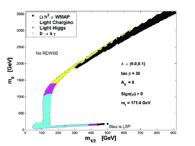
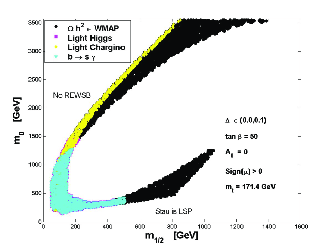
Figure 2: The allowed parameter space in the $m_{0}-m_{1/2}$ plane, under the $1\sigma$ WMAP3 constraint of Eq.(34) in extended mSUGRA for the case $A_{0}=0$, $\tan\beta=(30,50)$ (upper,lower), sign($\mu>0$), $m_{t}=171.4$ GeV, $m_{1/2}\in(0,1.5)$TeV and $m_{0}\in(0,3.5)$TeV, and $\Delta$ in the range (0.0, 0.1). Regions eliminated by the light chargino mass constraint, by the light Higgs mass constraint, and by the $b\to s+\gamma$ constraint are also exhibited.

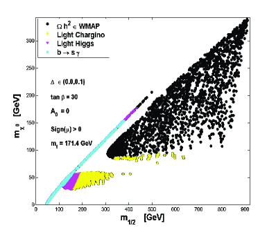
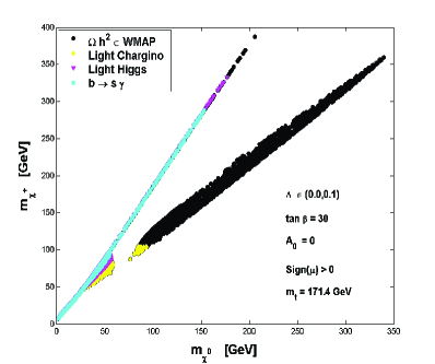
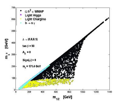
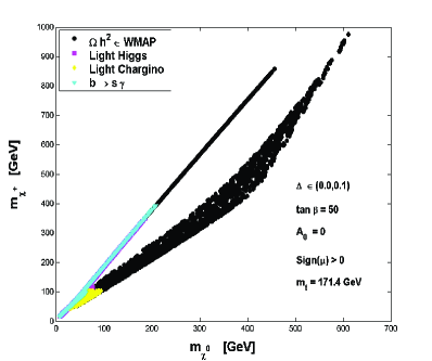
Figure 3: The allowed parameter space in the $m_{\chi^{0}}-m_{1/2}$ plane and in the $m_{\chi^{+}}-m_{\chi^{0}}$ plane, under the $1\sigma$ WMAP3 constraint of Eq.(34) in extended mSUGRA for the same data set as in Fig.(2). These plots exhibit the phenomenon of scaling and its breakdown and in particular for the ratio $m_{\chi^{+}}/m_{\chi^{0}}$ as discussed in the text.

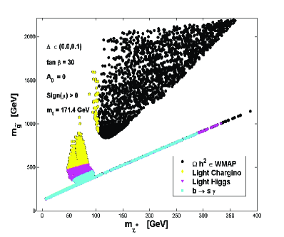
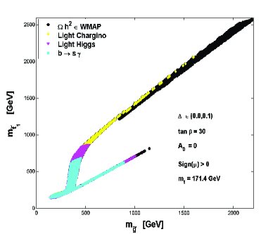
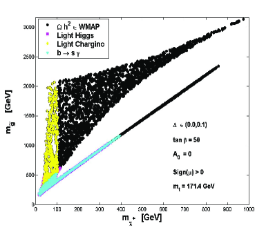
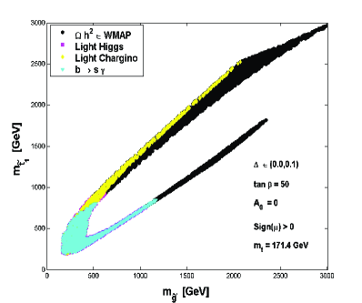
Figure 4: The allowed parameter space in the $m_{\tilde{g}}-m_{\chi^{+}}$ plane and in the $m_{\tilde{t}_{1}}-m_{\tilde{g}}$ plane, under the $1\sigma$ WMAP3 constraint of Eq.(34) in extended mSUGRA for the same data set as in Fig.(2).

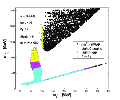
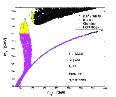
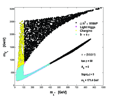
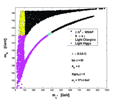
Figure 5: The allowed parameter space in the $m_{\tilde{t}_{1}}-m_{\chi^{+}}$ plane and in the $m_{h}-m_{\chi^{+}}$ plane, under the $1\sigma$ WMAP3 constraint of Eq.(34) in extended mSUGRA for the same data set as in Fig.(2).

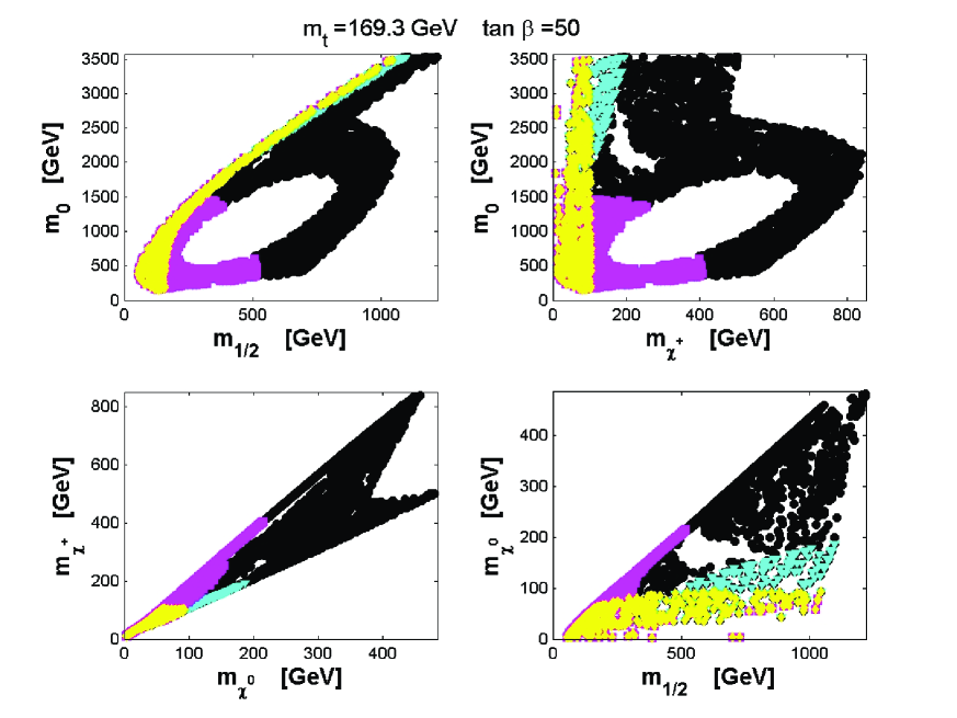
Figure 6: An analysis for the case when $m_{t}=169.3$ GeV which is $1\sigma$ below the central value, and $\tan\beta=50$ when all other parameters and constraints are the same as in Fig.(2).

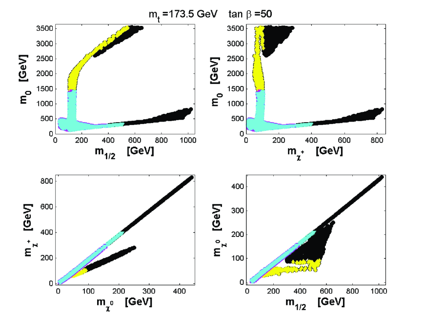
Figure 7: An analysis for the case when $m_{t}=173.5$ GeV which is $1\sigma$ above the central value, and $\tan\beta=50$ when all other parameters and constraints are the same as in Fig.(2).

References

- [1] For a recent work on the direct empirical evidence for the existence of dark matter in galaxies see, D. Clowe, M. Bradac, A. H. Gonzalez, M. Markevitch, S. W. Randall, C. Jones and D. Zaritsky, [astro-ph/0608407].
- [2] B. Körs and P. Nath, Phys. Lett. B 586, 366 (2004) [hep-ph/0402047].
- [3] B. Körs and P. Nath, JHEP 0412 (2004) 005 [hep-ph/0406167].
- [4] B. Körs and P. Nath, JHEP 0507, 069 (2005) [hep-ph/0503208].
- [5] B. Körs and P. Nath, [hep-ph/0411406]; MIT-CTP-3544. Proceedings of 10th International Symposium on Particles, Strings and Cosmology (PASCOS 04), Boston, Massachusetts, 16-22 Aug 2004. Published in *Boston 2004, Particles, strings and cosmology* 437-447.
- [6] D. Feldman, Z. Liu and P. Nath, Phys. Rev. Lett. 97, 021801 (2006) [hep-ph/0603039].
- [7] D. Feldman, Z. Liu and P. Nath, JHEP 0611, 007 (2006) [hep-ph/0606294].
- [8] P. Anastasopoulos, M. Bianchi, E. Dudas and E. Kiritsis, JHEP 0611, 057 (2006) [hep-th/0605225]. P. Anastasopoulos, T. P. T. Dijkstra, E. Kiritsis and A. N. Schellekens, Nucl. Phys. B 759, 83 (2006) [hep-th/0605226].
- [9] P. Nath, Phys. Rev. Lett. 76, 2218 (1996) [hep-ph/9512415].
- [10] M. Cvetic and P. Langacker, Mod. Phys. Lett. A 11 (1996) 1247 [hep-ph/9602424]; A.E. Farragi and M. Masip, Phys. Lett. B 388 (1996) 524 [hep-ph/9604302]; D. A. Demir, G. L. Kane and T. T. Wang, Phys. Rev. D 72, 015012 (2005) [hep-ph/0503290].
- [11] D. M. Ghilencea, L. E. Ibanez, N. Irges and F. Quevedo, JHEP 0208 (2002) 016; D. M. Ghilencea, Nucl. Phys. B 648 (2003) 215.
- [12] L. E. Ibanez, F. Marchesano and R. Rabadan, JHEP 0111 (2001) 002; R. Blumenhagen, V. Braun, B. Körs and D. Lüst, [hep-th/0210083]; I. Antoniadis, E. Kiritsis, J. Rizos and T. N. Tomaras, Nucl. Phys. B 660, 81 (2003); C. Coriano’, N. Irges and E. Kiritsis, Nucl. Phys. B 746, 77 (2006) [arXiv:hep-ph/0510332].
- [13] G. R. Dvali and A. Pomarol, Phys. Rev. Lett. 77, 3728 (1996) [hep-ph/9607383].
- [14] I. Antoniadis and S. Dimopoulos, Nucl. Phys. B 715, 120 (2005) [hep-th/0411032].
- [15] B. Körs and P. Nath, Nucl. Phys. B 711, 112 (2005) [hep-th/0411201].
- [16] P. Fayet and J. Iliopoulos, Phys. Lett. B 51, 461 (1974).
- [17] J. Hisano, S. Matsumoto and M. M. Nojiri, Phys. Rev. Lett. 92, 031303 (2004) [hep-ph/0307216]; K. Y. Choi and L. Roszkowski, AIP Conf. Proc. 805, 30 (2006) [hep-ph/0511003].
- [18] B. Holdom, Phys. Lett. B 166, 196 (1986).
- [19] A. Leike, Phys. Rept. 317, 143 (1999) [hep-ph/9805494].
- [20] D. Z. Freedman and B. Körs, JHEP 0611, 067 (2006) [hep-th/0509217]. H. Elvang, D. Z. Freedman and B. Körs, JHEP 0611, 068 (2006) [hep-th/0606012].
- [21] W. J. Marciano, Phys. Rev. D 60, 093006 (1999).
- [22] [ALEPH Collaboration], Phys. Rept. 427, 257 (2006) [hep-ex/0509008].
- [23] P. Nath and M. Yamaguchi, Phys. Rev. D 60, 116004 (1999) [hep-ph/9902323].
- [24] J. Kumar and J. D. Wells, [hep-ph/0606183].
- [25] W. F. Chang, J. N. Ng and J. M. S. Wu, Phys. Rev. D 74, 095005 (2006) [hep-ph/0608068].
- [26] K. Griest and D. Seckel, Phys. Rev. D 43, 3191 (1991).
- [27] A. H. Chamseddine, R. Arnowitt and P. Nath, Phys. Rev. Lett. 49 (1982) 970; R. Barbieri, S. Ferrara and C. A. Savoy, Phys. Lett. B 119 (1982) 343; L. J. Hall, J. D. Lykken and S. Weinberg, Phys. Rev. D 27 (1983) 2359; P. Nath, R. Arnowitt and A. H. Chamseddine, Nucl. Phys. B 227 (1983) 121.
- [28] J. R. Ellis, K. A. Olive, Y. Santoso and V. C. Spanos, Phys. Lett. B 565, 176 (2003) [hep-ph/0303043]; U. Chattopadhyay, A. Corsetti and P. Nath, Phys. Rev. D 68 (2003) 035005 [hep-ph/0303201]; H. Baer and C. Balazs, JCAP 0305, 006 (2003) [hep-ph/0303114]; H. Baer, C. Balazs, A. Belyaev, T. Krupovnickas and X. Tata, JHEP 0306, 054 (2003) [hep-ph/0304303]; A. B. Lahanas and D. V. Nanopoulos, Phys. Lett. B 568 (2003) 55 [hep-ph/0303130]; C. Munoz, Int. J. Mod. Phys. A 19 (2004) 3093 [hep-ph/0309346]; M. Battaglia, A. De Roeck, J. R. Ellis, F. Gianotti, K. A. Olive and L. Pape, Eur. Phys. J. C 33, 273 (2004) [hep-ph/0306219]; H. Baer, A. Mustafayev, S. Profumo, A. Belyaev and X. Tata, JHEP 0507 (2005) 065 [hep-ph/0504001]; H. Baer, A. Mustafayev, E. K. Park, S. Profumo and X. Tata, JHEP 0604, 041 (2006) [hep-ph/0603197]; J. R. Ellis, K. A. Olive, Y. Santoso and V. C. Spanos, JHEP 0605 (2006) 063 [hep-ph/0603136]; A. De Roeck, J. R. Ellis, F. Gianotti, F. Moortgat, K. A. Olive and L. Pape, [hep-ph/0508198]; V. Khotilovich, R. Arnowitt, B. Dutta and T. Kamon, Phys. Lett. B 618 (2005) 182 [hep-ph/0503165]; G. Belanger, F. Boudjema, S. Kraml, A. Pukhov and A. Semenov, Phys. Rev. D 73 (2006) 115007 [hep-ph/0604150]; G. B. Gelmini and P. Gondolo, Phys. Rev. D 74 (2006) 023510 [hep-ph/0602230]; M. E. Gomez, T. Ibrahim, P. Nath and S. Skadhauge, Phys. Rev. D 72 (2005) 095008 [hep-ph/0506243]; T. Nihei, Phys. Rev. D 73 (2006) 035005 [hep-ph/0508285]; S. F. King and J. P. Roberts, [hep-ph/0603095].
- [29] V. Barger, C. Kao, P. Langacker and H. S. Lee, Phys. Lett. B 600, 104 (2004) [hep-ph/0408120]; S. Nakamura and D. Suematsu, [hep-ph/0609061]; S. Profumo and A. Provenza, [hep-ph/0609290]; A. Provenza, M. Quiros and P. Ullio, [hep-ph/0609059]; B. de Carlos and J. R. Espinosa, Phys. Lett. B 407, 12 (1997) [hep-ph/9705315].
- [30] A. Djouadi, M. Drees and J. L. Kneur, Phys. Lett. B 624, 60 (2005) [hep-ph/0504090]; A. Djouadi, M. Drees and J. L. Kneur, JHEP 0603, 033 (2006) [hep-ph/0602001].
- [31] D. N. Spergel et al., [astro-ph/0603449].
- [32] G. Abbiendi et al. [OPAL Collaboration], Eur. Phys. J. C 35, 1 (2004) [hep-ex/0401026].
- [33] R. Barate et al. [LEP Working Group for Higgs boson searches], Phys. Lett. B 565, 61 (2003) [hep-ex/0306033].
- [34] The ALEPH, DELPHI, L3 and OPAL Collaborations, LHWG-Note 2005-01.
-
[35]
E. Barberio et al. [Heavy Flavor Averaging Group (HFAG)],
[hep-ex/0603003].
http://www.slac.stanford.edu/xorg/hfag/ - [36] G. Degrassi, P. Gambino and G. F. Giudice, JHEP 0012, 009 (2000) [hep-ph/0009337]; H. Baer, M. Brhlik, D. Castano and X. Tata, Phys. Rev. D 58, 015007 (1998) [hep-ph/9712305]; M. Carena, D. Garcia, U. Nierste and C. E. M. Wagner, Phys. Lett. B 499, 141 (2001) [hep-ph/0010003]; D. A. Demir and K. A. Olive, Phys. Rev. D 65, 034007 (2002) [hep-ph/0107329]; A. Buras, P. Chankowski, J. Rosiek and L. Slawianowska, Nucl. Phys. B659 (2003) 3-78 [hep-ph/0210145]; M. E. Gomez, T. Ibrahim, P. Nath and S. Skadhauge, Phys. Rev. D 74 (2006) 015015 [hep-ph/0601163]; G. Degrassi, P. Gambino and P. Slavich, [hep-ph/0601135].
- [37] G. Belanger, F. Boudjema, A. Pukhov and A. Semenov, [hep-ph/0607059]; G. Belanger, F. Boudjema, A. Pukhov and A. Semenov, Comput. Phys. Commun. 174, 577 (2006) [hep-ph/0405253]; G. Belanger, F. Boudjema, A. Pukhov and A. Semenov, Comput. Phys. Commun. 149 (2002) 103 [hep-ph/0112278].
- [38] A. Djouadi, J. L. Kneur and G. Moultaka, [hep-ph/0211331].
- [39] J. Edsjo and P. Gondolo, Phys. Rev. D 56, 1879 (1997) [hep-ph/9704361]; J. Edsjo, M. Schelke, P. Ullio and P. Gondolo, JCAP 0304, 001 (2003) [hep-ph/0301106]; P. Gondolo, J. Edsjo, P. Ullio, L. Bergstrom, M. Schelke and E. A. Baltz, JCAP 0407, 008 (2004) [astro-ph/0406204].
- [40] F. E. Paige, S. D. Protopopescu, H. Baer and X. Tata, [hep-ph/0312045].
- [41] H. Baer, C. Balazs, A. Belyaev, T. Krupovnickas and X. Tata, JHEP 0306, 054 (2003) [hep-ph/0304303]; H. Baer, A. Belyaev, T. Krupovnickas and J. O’Farrill, JCAP 0408, 005 (2004) [hep-ph/0405210]; Y. Mambrini and E. Nezri, [hep-ph/0507263]; M. M. Nojiri, G. Polesello and D. R. Tovey, JHEP 0603, 063 (2006) [hep-ph/0512204]; E. A. Baltz, M. Battaglia, M. E. Peskin and T. Wizansky, [hep-ph/0602187].
- [42] W. de Boer, I. Gebauer, M. Niegel, C. Sander, M. Weber, V. Zhukov and K. Mazumdar, CERN-CMS-NOTE-2006-113.
- [43] H. Baer, T. Krupovnickas and X. Tata, JHEP 0307, 020 (2003) [hep-ph/0305325]; V. M. Abazov et al. [D0 Collaboration], [hep-ex/0605009]; M. Carena, D. Hooper and P. Skands, Phys. Rev. Lett. 97, 051801 (2006) [hep-ph/0603180].
- [44] P. Nath and R. Arnowitt, Phys. Rev. Lett. 70, 3696 (1993) [hep-ph/9302318].
- [45] T. E. W. Group, [hep-ex/0608032].
- [46] P. Nath, J. z. Wu and R. Arnowitt, Phys. Rev. D 52, 4169 (1995) [hep-ph/9502388]; B. Allanach, S. Kraml and W. Porod, [hep-ph/0207314], J. R. Ellis, K. A. Olive, Y. Santoso and V. C. Spanos, Phys. Rev. D 69, 095004 (2004) [hep-ph/0310356]; M. E. Gomez, T. Ibrahim, P. Nath and S. Skadhauge, Phys. Rev. D 70, 035014 (2004) [hep-ph/0404025]; J. R. Ellis, S. Heinemeyer, K. A. Olive and G. Weiglein, JHEP 0502, 013 (2005) [hep-ph/0411216]; B. C. Allanach and C. G. Lester, Phys. Rev. D 73, 015013 (2006) [hep-ph/0507283]; A. Djouadi, M. Drees and J. L. Kneur, JHEP 0603, 033 (2006) [hep-ph/0602001].
- [47] K. L. Chan, U. Chattopadhyay and P. Nath, Phys. Rev. D 58, 096004 (1998) [hep-ph/9710473].
- [48] R. Arnowitt and P. Nath, Phys. Rev. Lett. 69, 725 (1992).