On two- and three-body descriptions of hybrid mesons

Abstract

Hybrid mesons are exotic mesons in which the color field is not in its ground state. Their understanding deserves interest from a theoretical point of view, because it is intimately related to nonperturbative aspects of QCD. In this work, we analyze and compare two different descriptions of hybrid mesons, namely a two-body $q\bar{q}$ system with an excited string, or a three-body $q\bar{q}g$ system. In particular, we show that the constituent gluon approach is equivalent to an effective excited string in the heavy hybrid sector. Instead of a numerical resolution, we use the auxiliary field technique. It allows to find simplified analytical mass spectra and wave functions, and still leads to reliable qualitative predictions. We also investigate the light hybrid sector, and found a mass for the lightest hybrid meson which is in satisfactory agreement with lattice QCD and some effective models.

I Introduction

The study of hybrid mesons deserves much interest in theoretical as well as in experimental particle physics. From a theoretical point of view, these particles are interpreted as mesons in which the color field is in an excited state. Numerous lattice QCD calculations have been devoted to the study of hybrid mesons, in particular to the energy levels of the gluonic field Juge ; Juge2 and to the properties of the $1^{-+}$ state, which is the lightest hybrid with exotic quantum numbers (see Refs. Nel02 ; Liu06 for useful references). On the experimental side, we can mention the recently observed $\pi_{1}(1600)$ Ada98 , $\pi_{1}(2000)$ Lu and $Y(4260)$ aub05 , which could be either hybrid mesons, or tetraquark states Klem04 .

Apart from lattice QCD, hybrid mesons have been studied with effective models for a long time. For example, we can quote the flux tube model flux , models with constituent gluons horn ; constg , or the MIT bag model bag . In potential models, to which our paper is devoted, there are two main approaches. In the first one, the quark and the antiquark are linked by a string, or flux tube, which simulates the exchange of gluons responsible for the confinement. If the string is in the ground state, it reduces to the usual linear confinement potential for heavy quarks, and to a more general flux tube model for light quarks, where the dynamics of the string cannot be neglected laco89 . In this stringy picture, it is possible for the flux tube to fluctuate at the quantum level, and thus to be in an excited state. These string excitations are analog to the gluon field excitations in full QCD. They have been studied for example in Refs. Allen:1998wp ; luscher . In the second approach, it is assumed that the hybrid meson is a three-body system, formed of a quark, an antiquark, and a constituent gluon, which represents the gluonic excitation. Two fundamental strings then link the gluon to the quark and to the antiquark. This picture has been studied in Ref. constg , but also in more recent works Kalashnikova:2002tg ; hyb1 .

Nowadays, the spinless Salpeter Hamiltonian (SSH) with a linear confinement is a widely used and successful framework to compute hadron spectra in potential models (see previous references). Since its kinetic operator is a semi-relativistic one, most of the results are numerically obtained. However, the auxiliary field (AF) technique, also known as the einbein field method, allows to greatly simplify the calculations Sem03 ; Simo1 . In a previous work hyb1 , it is shown that the AF method leads to analytic solutions for the eigenvalues and wave functions of the two-body SSH. Even if they are approximations, these solutions are qualitatively in agreement with well-known experimental facts, the Regge trajectories for example. The AF technique was also applied to the case of hybrid mesons with a constituent gluon and two static quarks. This model is able to reproduce some lattice results concerning the gluonic energy levels and the heavy hybrid spectroscopy. Moreover, it suggests a correspondence between the excited flux tube and the constituent gluon approaches hyb1 . The purpose of the present paper is now to apply the AF technique to the full $q\bar{q}g$ system, without demanding that the quark and the antiquark are static, in order to obtain formula which are valid for arbitrary quark mass. Moreover, we will further investigate the links between the excited string and the constituent gluon pictures. Eventually, we will show that these approaches are equivalent for heavy quarks. Our formalism will also allow us to study whether this equivalence is modified in the light quark sector or not.

Our paper is organized as follows. In Sec. II, we review the main properties of the AF method by applying it to the simple case of mesons. In Sec. III, we discuss the excited flux tube model of hybrid mesons. Then, we analytically solve the $q\bar{q}g$ three-body problem corresponding to hybrid mesons with a constituent gluon in Sec. IV, and give some physical results concerning their mass and structure. In Sec. V, we derive the effective quark-antiquark potential for the $q\bar{q}$ system within a hybrid meson, and we discuss its links to the excited string picture. Finally, we compare our results to lattice QCD in Sec. VI, and draw some conclusions in Sec. VII.

II Mesons and auxiliary fields

A system made of two hadrons interacting through a linear confinement can be described by the following SSH

$$H=\sqrt{\bm{p}^{\,2}+m^{2}_{1}}+\sqrt{\bm{p}^{\,2}+m^{2}_{2}}+ar,$$ (1)

where $\bm{p}^{\,2}_{1}=\bm{p}^{\,2}_{2}=\bm{p}^{\,2}$ since we work in the center of mass frame. The linear confinement can be understood as the static contribution of a straight string, or flux tube, of tension $a$, linking the quark and the antiquark laco89 . In order to get rid of the square roots appearing in Hamiltonian (1), let us now introduce three AF: Two for the quarks, denoted $\mu_{i}$, and one for the potential, $\nu$. Hamiltonian (1) then becomes

$$H(\mu_{i},\nu)=\frac{\bm{p}^{\,2}+m^{2}_{1}}{2\mu_{1}}+\frac{\mu_{1}}{2}+\frac{\bm{p}^{\,2}+m^{2}_{2}}{2\mu_{2}}+\frac{\mu_{2}}{2}+\frac{a^{2}r^{2}}{2\nu}+\frac{\nu}{2}.$$ (2)

Although being formally simpler, $H(\mu_{i},\nu)$ is equivalent to $H$ up to the elimination of the AF thanks to the constraints

$$\delta_{\mu_{i}}H(\mu_{i},\nu) = 0\ \Rightarrow\ \mu_{i0}=\sqrt{\bm{p}^{\,2}+m^{2}_{i}},$$ (3a)

$$\delta_{\nu}H(\mu_{i},\nu) = 0\ \Rightarrow\ \nu_{0}=ar.$$ (3b)

It is worth mentioning that $\left\langle\mu_{i0}\right\rangle$ can be seen as a dynamical mass of the quark whose current mass is $m_{i}$, while $\left\langle\nu\right\rangle$ is in this case the static string energy Fab1 . Relations (3) show that the AF are, strictly speaking, operators. However, the calculations are considerably simplified if the AF are considered as real numbers, and finally eliminated by a minimization of the masses Sem03 . The extremal values of $\mu_{i}$ and $\nu$, considered as numbers, are logically close to the values $\left\langle\mu_{i0}\right\rangle$ and $\left\langle\nu_{0}\right\rangle$ given by relations (3). This procedure leads to a spectrum which is an upper bound of the “true spectrum” (computed without AF), the differences being about $10\%$ Fab3 .

Using the AF, Hamiltonian (1) turns out to be formally a simple nonrelativistic harmonic oscillator (2). Its mass spectrum and wave functions read

$$M(\mu_{i},\nu)=\omega(2n+\ell+3/2)+\frac{m^{2}_{1}}{2\mu_{1}}+\frac{m^{2}_{2}}{2\mu_{2}}+\frac{\mu_{1}+\mu_{2}+\nu}{2},$$ (4)

$$\psi=\phi_{n,\ell}(\beta^{1/2}r)Y^{m}_{\ell}(\theta,\varphi),$$ (5)

where

$$\omega=\sqrt{a^{2}/\tilde{\mu}\nu},\quad\beta=\sqrt{\tilde{\mu}a^{2}/\nu},\quad\tilde{\mu}=\frac{\mu_{1}\mu_{2}}{\mu_{1}+\mu_{2}},$$ (6)

and where $\phi_{n,\ell}(\beta^{1/2}r)$ is a normalized radial eigenfunction of the three dimensional harmonic oscillator.

In the special case of a light meson, one can set $m_{1}=m_{2}=0$. Then $\mu_{1}=\mu_{2}=\mu$, and one obtains after the elimination of the AF hyb1

$$M^{2}_{ll}=8a(2n+\ell+3/2).$$ (7)

At large angular momentum, it appears that the square mass increases linearly with $\ell$. Thus, our solution qualitatively reproduces the Regge trajectories, which are the best known experimental fact concerning the light meson spectroscopy. The Regge slope is here given by $8a$ instead of $2\pi a$, which is the exact value of the Regge slope in the flux tube model laco89 . This is related to the AF technique itself which gives good qualitative results, but overestimates the masses. More precisely, the error on the exact value increases with the number of AF introduced, as shown in Ref. hyb1 . As a check of this point, we can mention that with only one AF, the Regge slope can be computed to be $7a$ qse . What can be done to cure this artifact of the AF method is to rescale $a$: as we know that the exact Regge slope is around $2\pi\sigma$, with the standard value $\sigma\approx 0.2$ GeV², let us set $a=2\pi\sigma/8$. Then, a mass formula such as expression (7) is able to correctly reproduce the experimental Regge slope of the mesons laco89 . In the following, a rescaling of the string tension will be used to improve the results given by the AF calculations.

An other interesting case is a system composed of a light quark and of a heavy quark. One finds that, for such a system hyb1 ,

$$(M_{hl}-m_{2})^{2}=4a(2n+\ell+3/2).$$ (8)

The Regge slope for a heavy-light meson is half of the one for a light-light meson. As it was shown in Ref. Ols94 , it is in agreement with experimental observations. Again, the correct Regge slope in this case is not $4a$ but $\pi a$ Ols94 . With the same rescaling as above, $a=\pi\sigma/4$, the approximate result (8) can be greatly improved.

Equation (8) can also be applied to a special type of heavy hybrid mesons called hybrid gluelumps, that is a pointlike heavy $q\bar{q}$ pair with mass $m_{q\bar{q}}$ bound to a constituent gluon. We have then

$$(M_{hyb}-m_{q\bar{q}})^{2}=4\lambda(2n+\ell)+6\lambda,$$ (9)

where $\lambda$ is the string tension between the gluon and the $q\bar{q}$ pair. Note that $n$ and $\ell$ are the quantum numbers of the gluon, since the dynamics of the heavy $q\bar{q}$ pair can be neglected. Such a Regge-like behavior for heavy hybrid mesons has been obtained numerically in Ref. gluelump .

III Hybrid mesons and the excited flux tube

It is generally accepted that the static potential between the quark and the antiquark in an usual meson is compatible with a funnel potential,

$$V_{F}=ar-\frac{4\alpha_{S}}{3r},$$ (10)

where $\alpha_{S}$ is the strong coupling constant. The Coulomb part comes from one-gluon exchange process, while the $ar$ part is a pure confinement: it corresponds to the (classical) energy of a straight string linking the quark and the antiquark, and whose energy density is $a$. The description of the confining interaction in terms of such a string is an effective approach which can be derived from QCD dubi94 . Let us note that the spectrum obtained with potential (10) is in good agreement with experimental data for the light and heavy mesons truc . Typical values for the parameters fitting the lattice QCD data are $a\approx 0.2$ GeV², and $\alpha_{S}\approx 0.2$-0.3.

The nonabelian nature of QCD makes possible for a gluon to interact with other gluons. These kind of self-interactions allow the gluonic field to be in an excited state, like it is expected to be the case in hybrid mesons. These excitations can be translated in a stringy language by computing the energy spectrum of a quantum string, the string fluctuations corresponding to the color field excitations. The string energy, and consequently the potential energy between the static quark and antiquark is then given by arvi

$$V(r)=\sqrt{a^{2}r^{2}+2\pi aN+{\cal E}^{2}},$$ (11)

where $N$ is the string excitation number. Let us note that the values of this number are constrained by the fact that the quantity under the square root must be positive.

It is generally accepted in string theory that ${\cal E}^{2}=-2\pi a(D-2)/24$, with $D$ the dimension of space. Together with $D=26$, this value indeed ensures that the Lorentz invariance is still present at the quantum level. It is worth mentioning that we are here dealing with effective models of QCD with $D=4$: our string is not a fundamental object but an effective one arising from the exchanged gluons. Consequently, it is clear that such an effective model could be characterized by a nonstandard value of ${\cal E}$. Moreover, a potential model like the SSH is a priori noncovariant since the potentials which are used are instantaneous: the Lorentz invariance is already broken at the classical level, so one does not need to restrict ${\cal E}$ to the usual value. From an effective model point of view, the best interpretation to give to ${\cal E}$ seems thus the one proposed in Ref. brink , where it is shown that it represents the zero point energy of the transverse string fluctuations. In a QCD model, this could be the zero point energy of the gluonic field. We will turn to this interpretation later, to see that it is indeed compatible with our results. Let us note that for large $r$, potential (11) is approximately equal to

$$V(r)=ar+\frac{\pi}{r}\left(N_{L}+\frac{{\cal E}^{2}}{2\pi a}\right).$$ (12)

In $D=4$, the usual string theory states that ${\cal E}^{2}/2\pi a=-1/12$: we recover in this limit the well-known universal Lüscher term luscher . In formula (12), the minimal allowed value for $N_{L}$ is zero. In this case, $V(r)$ is expected to reproduce the funnel potential and thus represents the interaction of a quark and an antiquark in an ordinary meson.

We can apply the auxiliary field formalism to compute a hybrid meson spectrum in the same way as it was done in the previous section for mesons. However, the potential to use is now given by formula (11) instead of the usual $ar$. Then, the hybrid masses are given by

$$M_{hyb}(\mu_{i},\nu)=M(\mu_{i},\nu)+\frac{2\pi aN+{\cal E}^{2}}{2\nu},$$ (13)

with $M(\mu_{i},\nu)$ given by Eq. (4). Because of the new term, $\nu$ is more complex to eliminate. Nevertheless, we can readily compute that, in the case of a heavy hybrid meson with the quark and the antiquark of the same mass, we have $M(\mu_{i},\nu)\approx 2m+\nu/2$ (the dynamical contribution of the quark and of the antiquark is neglected), and consequently,

$$(M_{hyb}-2m)^{2}\approx 2\pi aN+{\cal E}^{2}.$$ (14)

This is a kind of Regge trajectory with respect to the string excitation number $N$. It is interesting to notice that this formula is analog to the result of Eq. (9) concerning the heavy hybrid mesons, with $m_{q\bar{q}}=2m$, $\lambda=2a$ and the proper rescaling $a=\pi\sigma/4$ (these values for $m_{q\bar{q}}$ and $\lambda$ will be justified in Sec. IV.2). The quantum numbers of the gluon, $(2n+\ell)$, are replaced by $N$ the string excitation number, and the square zero point energy of the system, $6\lambda$, is now replaced by ${\cal E}^{2}$, the square zero point energy of the string fluctuations. This correspondence is a first hint that the description of heavy hybrid mesons in terms of a constituent gluon or of an excited string possesses a similar physical content, expressed in terms of two different degrees of freedom, namely a gluon or a string excitation. We will further investigate this correspondence in the following.

IV Hybrid mesons with constituent gluons

IV.1 The three-body problem

In this picture, it is assumed that the excitations of the gluon field can be described by a constituent gluon interacting with the quark-antiquark pair. This pair is thus in a color octet in order for the hybrid meson to be a colorless object. Assuming the Casimir scaling hypothesis, which seems to be confirmed by several models scaling , it can be shown that the confinement is no more a Y-junction like in a baryon but two fundamental strings linking each quarks to the gluon gluelump . Neglecting all the short-range interactions, the three-body SSH is thus

$$H=\sum_{i=q,\bar{q},g}\sqrt{\bm{p}^{2}_{i}+m^{2}_{i}}+\sum_{j=q,\bar{q}}a|\bm{x}_{j}-\bm{x}_{g}|,$$ (15)

with $m_{g}=0$. Introducing the AF, we obtain, in analogy with Hamiltonian (2),

$$H(\mu_{i},\nu_{i}) = \sum_{i=q,\bar{q},g}\left[\frac{\bm{p}^{2}_{i}+m^{2}_{i}}{2\mu_{i}}+\frac{\mu_{i}}{2}\right]$$ (16)

$$+\sum_{j=q,\bar{q}}\left[\frac{a^{2}(\bm{x}_{j}-\bm{x}_{g})^{2}}{2\nu_{j}}+\frac{\nu_{j}}{2}\right].$$

We can then apply the procedure described in Ref. coqm , where we solved the three-body covariant oscillator quark model by an appropriate change of variables.

First of all, we will replace the quark coordinates $\bm{x}_{i}=\left\{\bm{x}_{g},\bm{x}_{q},\bm{x}_{\bar{q}}\right\}$ by $\bm{x}^{\prime}_{k}=\left\{\bm{R},\bm{r},\bm{y}\right\}$, with the center of mass defined as

$$\bm{R}=\frac{\mu_{g}\bm{x}_{g}+\mu_{q}\bm{x}_{q}+\mu_{\bar{q}}\bm{x}_{\bar{q}}}{\mu_{t}}.$$ (17)

$\mu_{t}=\mu_{g}+\mu_{q}+\mu_{\bar{q}}$ and $\{\bm{r},\bm{y}\}$ are two relative coordinates. The change of coordinates is made via a matrix $Q$, thanks to the relation $\bm{x}_{i}=Q_{ik}\bm{x}^{\prime}_{k}$. Let us note that the invariance of the Poisson brackets demands that $\bm{p}_{i}=\left(Q^{-1}\right)^{\rm{T}}_{ik}\bm{p}^{\prime}_{k}$, with $\bm{p}^{\prime}_{i}=\left\{\bm{P},\bm{p},\bm{p}_{y}\right\}$. We define

$$Q=\left(\begin{array}[]{ccc}1&A&B\\ 1&C&D\\ 1&E&F\end{array}\right),$$ (18)

and choose to impose the constraints

$$D=F,\quad C=E+1,$$ (19)

in order to have a clear physical meaning for $\bm{r}$, that is simply

$$\bm{r}=\bm{x}_{q}-\bm{x}_{\bar{q}}.$$ (20)

Moreover, we ask that

$$A = -\frac{\mu_{q}}{\mu_{g}}C-\frac{\mu_{\bar{q}}}{\mu_{g}}E,$$ (21a)

$$B = -\frac{\mu_{q}}{\mu_{g}}D-\frac{\mu_{\bar{q}}}{\mu_{g}}F,$$ (21b)

$$E = -\frac{\mu_{q}}{\mu_{q}+\mu_{\bar{q}}},$$ (21c)

$$F = \frac{\mu_{g}}{\sqrt{\mu_{t}(\mu_{q}+\mu_{\bar{q}})}}.$$ (21d)

Constraints (21a) and (21b) are consequences of the definition (17): they allow the vanishing of the terms in $\bm{P}\cdot\bm{p}$ and $\bm{P}\cdot\bm{p}_{y}$ when Hamiltonian (16) is rewritten in the new coordinates. Equation (21c) ensures that the cross product $\bm{p}\cdot\bm{p}_{y}$ is equal to zero too. In the general case, these constraints are not sufficient to eliminate the terms in $\bm{r}\cdot\bm{y}$. However, if $m_{q}=m_{\bar{q}}=m$, that is to say that $\mu_{q}=\mu_{\bar{q}}=\mu$ and $\nu_{q}=\nu_{\bar{q}}=\nu$, these terms vanish. In what follows, we will thus restrict ourselves to the case of a quark and an antiquark with the same mass. In the center of mass frame, $\bm{P}=\bm{0}$, the Hamiltonian (16) becomes

$$H(\mu_{i},\nu)=\frac{\bm{p}^{2}}{2\tilde{\mu}}+\frac{\bm{p}^{2}_{y}}{2\mu_{g}}+\frac{1}{2}\Omega_{r}\bm{r}^{2}+\frac{1}{2}\Omega_{g}\bm{y}^{2}+\frac{m^{2}}{\mu}+\mu+\frac{\mu_{g}}{2}+\nu,$$ (22)

with

$$\Omega_{r}=\frac{a^{2}}{2\nu},\quad\Omega_{g}=\frac{a^{2}(\mu_{g}+2\mu)}{\mu\nu},$$ (23)

and $\tilde{\mu}=\mu/2$. As in Ref. coqm , our transformation leads to a Hamiltonian were all variables are separated. Actually, we have decoupled the three-body hamiltonian (15) into a sum of two Hamiltonians: one for the two-body quark-antiquark system, the $\bm{r}$ dependent part, and one for the gluon, the $\bm{y}$ dependent part. To confirm this point, let us mention that the mass term appearing with $\bm{p}^{2}$ is the reduced mass of the quark and the antiquark, and the one appearing with $\bm{p}^{2}_{y}$ is $\mu_{g}$. This nice feature is due to our choice of $F$, given by Eq. (21d). Moreover, $A=0$ when $\mu_{q}=\mu_{\bar{q}}$. This means that the gluon position is only given by a function of $\bm{y}$. But, this separation is only formal, since the AF still have to be eliminated. This will make appear the couplings between the three bodies.

Before doing this, we can remark that Hamiltonian (22) is the sum of two harmonic oscillators. The mass spectrum and wave functions are then easily obtained. They read

$$E(\mu_{i},\nu)=\omega_{r}(2n+\ell+3/2)+\omega_{g}({\cal N}+3/2)+\frac{m^{2}}{\mu}+\mu+\frac{\mu_{g}}{2}+\nu,$$ (24)

$$\psi = \psi_{q\bar{q}}(\bm{r})\times\psi_{g}(\bm{y})=\phi_{n,\ell}(\beta^{1/2}_{r}\,r)Y^{m}_{\ell}(\theta,\varphi)$$ (25)

$$\times\phi_{n_{y},\ell_{y}}(\beta^{1/2}_{y}\,y)Y^{m_{y}}_{\ell_{y}}(\theta_{y},\varphi_{y}),$$

and

$$\omega_{r}=\frac{a}{\sqrt{\mu\nu}},\quad\omega_{g}=a\sqrt{\frac{\mu_{g}+2\mu}{\mu\nu\mu_{g}}},$$ (26)

$$\beta_{r}=\tilde{\mu}\omega_{r},\quad\beta_{g}=\mu_{g}\omega_{y}.$$ (27)

For later convenience, we also defined

$${\cal N}=2n_{y}+\ell_{y}.$$ (28)

The allowed values for ${\cal N}$ are 0, 1, …It is worth noting that the state ${\cal N}=0$ does not correspond to an ordinary meson state (as in the case $N_{L}=0$ for the potential (12)), but to the hybrid meson ground state.

Formulas (24) and (25) are a generalization of the results of Ref. hyb1 , since in this last work the quark and the antiquark were assumed to be fixed and the dynamics of the system was actually a one-body problem. Here, we deal with the full three-body system. Using the well-known properties of the harmonic oscillator, it is easy to compute the quantities

$$\left\langle r^{2}\right\rangle=\frac{(2n+\ell+3/2)}{\beta_{r}},\quad\left\langle y^{2}\right\rangle=\frac{({\cal N}+3/2)}{\beta_{g}}.$$ (29)

They give information about the geometric configuration of the three bodies. The elimination of the AF has now to be performed by minimizing the energy (24) with respect to them. This problem leads to rather complex expressions in general, but can be simplified in the case of heavy and light hybrids.

IV.2 Heavy hybrid mesons

In this section, we will consider that $m\gg\sqrt{a}$ to obtain simple analytical formula. In this case, the quark and the antiquark are very heavy and we can set $\mu\approx m$. Formula (24) then reduces to

$$E(\mu_{g},\nu) = \frac{a}{\sqrt{m\nu}}(2n+\ell+3/2)+a\sqrt{\frac{2}{\nu\mu_{g}}}({\cal N}+3/2)$$ (30)

$$+2m+\frac{\mu_{g}}{2}+\nu.$$

Neglecting the excitation energy of the $q\bar{q}$ pair, we obtain

$$E(\mu_{g},\nu) \approx a\sqrt{\frac{2}{\nu\mu_{g}}}({\cal N}+3/2)+2m+\frac{\mu_{g}}{2}+\nu.$$ (31)

As $E(\mu_{g},\nu)$ is symmetric for the exchange $\mu_{g}\leftrightarrow 2\nu$, we can set

$$\mu_{g}\approx 2\nu$$ (32)

to simplify the energy formula (31). The constraint $\delta_{\nu}E(\nu)=0$ gives

$$\nu_{0}=\sqrt{\frac{a}{2}({\cal N}+3/2)},$$ (33)

$$(E-2m)^{2}=8a{\cal N}+12a.$$ (34)

This last mass formula is clearly analog to Eq. (9). The string tension is here $2a$ because the total string results in the superposition of the two fundamental strings linking the gluon to the quark and to the antiquark, in the limit of a pointlike $q\bar{q}$ pair with $m_{q\bar{q}}=2m$ (no interaction between the quarks).

As it was argued in a previous study using special relativity arguments scz , the geometrical configuration of a heavy hybrid meson is most likely to be a quark and an antiquark close to each other, with a gluon orbiting around the pair. In our model, it is easy to compute that in the ground state ($n=\ell={\cal N}=0$),

$$\left\langle r^{2}\right\rangle=\frac{3^{5/4}}{a^{3/4}\sqrt{2m}}\ <\ \left\langle y^{2}\right\rangle=\frac{3}{4a}.$$ (35)

The quark-antiquark separation is smaller than the distance between the gluon and the center of mass, in agreement with results of Ref. scz . This is the hybrid gluelump picture that we already mentioned in Sec. II, and which was studied in Ref. gluelump . In this case, it is also showed in Ref. hyb1 that the heavy hybrid masses are in agreement with lattice QCD calculations.

Let us point out that the results of this section are strictly valid in the limit $m\rightarrow\infty$, like in the case of static quarks which are considered in lattice QCD. Indeed, even if we set $m=5$ GeV, that is a value slightly above the $b$ quark mass, relation (35) is not true. We have in this case $\left\langle r^{2}\right\rangle\approx\left\langle y^{2}\right\rangle$.

IV.3 Light hybrid mesons

One of the nice features of our formalism is that it is well defined for vanishing quark masses. In this case we can assume that $\mu\approx\mu_{g}$, since the gluon, the quark and the antiquark are massless particles. Mass formula (24) then becomes

$$E(\mu,\nu)=\frac{a}{\sqrt{\mu\nu}}(2n+\ell+3/2)+a\sqrt{\frac{3}{\mu\nu}}({\cal N}+3/2)+\frac{3}{2}\mu+\nu.$$ (36)

The symmetry of Eq. (36) allows us to use the relation

$$3\mu=2\nu.$$ (37)

A numerical solution of mass formula (24) for $m=0$ gives $\mu/\mu_{g}=0.81$ and $3\mu/2\nu=0.93$ for the ground state, whatever the value of $a$, in quite good agreement with our approximations. Let us note that they are mostly valid when the excitation energies of the quarks and the gluon are similar.

After the minimization of $E$ with respect to $\nu$ we obtain

$$\nu_{0}=\sqrt{\frac{a}{2}\sqrt{\frac{3}{2}}(2n+\ell+3/2)+\frac{3a}{2\sqrt{2}}({\cal N}+3/2)},$$ (38)

$$E^{2}=4\sqrt{6}\left[a(2n+\ell+3/2)+a\sqrt{3}({\cal N}+3/2)\right].$$ (39)

This formula predicts that the light hybrid mesons should exhibit Regge trajectories at large $\ell$ like the usual light mesons. The trajectories corresponding to different values of ${\cal N}$ are parallel but differ in their intercept: two successive trajectories are separated by $2^{5/2}3a$.

Concerning the structure of these hybrid mesons, we can compute that in the ground state

$$\left\langle r^{2}\right\rangle=\frac{3}{2a}\sqrt{6}\ >\ \left\langle y^{2}\right\rangle=\frac{3}{2a}\frac{1}{\sqrt{2}}.$$ (40)

The larger quantity is now clearly the quark-antiquark separation. The light hybrid meson structure is thus rather different from the heavy hybrid meson one. In particular, the picture of a pointlike $q\bar{q}$ pair is no longer valid.

We can use formula (39) and (40) to estimate the mass of the lightest hybrid meson in our model. The ground state mass is given by $E_{0}=6.337\sqrt{a}$  GeV. In a first approximation, the total energy should be given by $E=E_{0}+\Delta E$ with

$$\Delta E=\left\langle\frac{\alpha_{S}}{6r}-\frac{3\alpha_{S}}{2r_{qg}}-\frac{3\alpha_{S}}{2r_{\bar{q}g}}\right\rangle$$ (41)

encoding the one gluon exchange processes at the lowest order horn . Thanks to relations (21), we have

$$\bm{x}_{g}-\bm{x}_{q}=-\sqrt{\frac{\mu_{t}}{\mu_{q}+\mu_{\bar{q}}}}\bm{y}-\frac{\bm{r}}{2}.$$ (42)

Assuming that $|\bm{x}_{g}-\bm{x}_{q}|\approx|\bm{x}_{g}-\bm{x}_{\bar{q}}|$ thanks to the symmetry of our problem, Eq. (40) implies

$$\left\langle r^{2}_{qg}\right\rangle=\left\langle r^{2}_{\bar{q}g}\right\rangle\approx\frac{\left\langle r^{2}\right\rangle}{4}+\frac{3\left\langle y^{2}\right\rangle}{2}=\frac{2.510}{a}.$$ (43)

Thus,

$$\Delta E\approx\frac{\alpha_{S}}{6\sqrt{\left\langle r^{2}\right\rangle}}-\frac{3\alpha_{S}}{\sqrt{\left\langle r_{qg}^{2}\right\rangle}}.$$ (44)

With the value $\alpha_{S}=0.4$, which was already successfully used in the description of light mesons instanton ; fulch , we find $\Delta E=-0.724\sqrt{a}$ and $E=5.613\sqrt{a}$. We already pointed out in Sec. II that the AF method gives qualitative results in agreement with observations, but overestimates the masses. The Regge slope is here $4\sqrt{6}a$. But we can expect that, at large $\ell$, the contribution of the constituent gluon can be neglected with respect to the contribution of the quark-antiquark pair. Then, the exact slope should be given by $2\pi a$ as in the meson case. As it is proposed in Sec. II, we can thus rescale the string tension and define $a=2\pi\sigma/4\sqrt{6}$, with $\sigma=0.2$ GeV² the physical string tension. We finally obtain

$$E=4.495\sqrt{\sigma}=2.010\ {\rm GeV}$$ (45)

for the lightest hybrid meson.

It is worth mentioning that several approaches, such as QCD in Coulomb gauge llanes , flux tube model merlin , and lattice QCD Bern97 , lead to the conclusion that the lightest hybrid meson mass is around $2$ GeV. Interestingly, this is close to the recently observed $\pi_{1}(2000)$ exotic state Lu . However, we stress that, since our model neglects the spin interactions, the energy (45) is only a rough estimation of the lightest hybrid mass. As formula (39) does not involve the spin quantum numbers, its ground state ( $n=\ell={\cal N}=0$) could have the following quantum numbers kala

$$J^{PC}=0^{\pm+},1^{\pm+},1^{\pm-},2^{\pm+}.$$ (46)

These eight states are clearly degenerate in our approach. Our estimation of the ground state mass should thus be regarded as a spin- averaged mass of the multiplet (46). The spin corrections are expected to contribute for at most $10\%$ of the total mass kala . Consequently, they have to be taken into account if one wants to make an accurate comparison with either lattice or experimental data.

It is interesting to mention that, in the flux tube model, the lowest hybrid states can have the following quantum numbers merlin :

$$J^{PC}=0^{\pm\mp},\,1^{\pm\pm},\,1^{\pm\mp},\,2^{\pm\mp}.$$ (47)

The multiplets predicted by the flux tube model and the constituent gluon approach are not identical: only six states on eight are in correspondence. The inclusion of spin interactions in both approaches would thus lead to different results, but a detailed comparison of these differences is out of the scope of this paper.

V Effective two-body potentials

After having studied the hybrid mesons as a three-body system, we would like to connect this model with a two-body description. More precisely, we would like to absorb the gluonic degree of freedom into an effective potential between the quark and the antiquark. To do this, we begin by averaging the three-body Hamiltonian (22) on the gluon wave function $\left|\psi_{g}\right\rangle$. We assume that

$$H_{q\bar{q}}(\mu_{i},\nu) = \left\langle\psi_{g}\right|H(\mu_{i},\nu)\left|\psi_{g}\right\rangle$$ (48)

$$= \frac{\bm{p}^{2}+m^{2}}{\mu}+\mu+\frac{1}{2}\Omega_{r}r^{2}+\omega_{g}({\cal N}+3/2)$$

$$+\frac{\mu_{g}}{2}+\nu.$$

The first two terms are the kinetic part of a two-body SSH. Consequently, the other terms are interpreted as the effective potential between the quark and the antiquark, i. e.

$$V_{q\bar{q}}(\mu_{i},\nu)=\frac{1}{2}\Omega_{r}r^{2}+\omega_{g}({\cal N}+3/2)+\frac{\mu_{g}}{2}+\nu.$$ (49)

This potential being still dependent of the AF, we have to carefully remove them. This will be done in the two special cases we treated previously, namely the light and heavy hybrid mesons.

V.1 Heavy hybrid mesons

When $\mu=m$, the potential (49) only depends on $\nu$ and $\mu_{g}$. But, following relation (32), $\mu_{g}=2\nu$. This allows to eliminate the gluonic degree of freedom and replace it by a stringy equivalent. Doing this, $\nu$ becomes the AF associated with an “effective” string linking the quark and the antiquark. We have

$$H_{q\bar{q}}(\nu)=2m+\frac{\bm{p}^{2}}{m}+V_{q\bar{q}}(\nu),$$ (50)

with

$$V_{q\bar{q}}(\nu)=\frac{a^{2}r^{2}+4a({\cal N}+3/2)}{4\nu}+2\nu.$$ (51)

The condition $\delta_{\nu}H_{q\bar{q}}(\nu)=0$ leads after replacement to

$$V_{q\bar{q}}=\sqrt{2}\sqrt{a^{2}r^{2}+4a({\cal N}+3/2)}.$$ (52)

The $\sqrt{2}$ factor is clearly unphysical, since the asymptotic form of $V_{q\bar{q}}$ should be $ar$ Allen:1998wp . Actually, it is due to the AF formalism itself, which overestimates the masses, and thus the potential energies too. As we argued in Sec. II, a rescaling of the string tension can be performed to find the correct expression. If we define $a=\sigma/\sqrt{2}$, we have

$$V_{q\bar{q}}=\sqrt{\sigma^{2}r^{2}+2^{5/2}\sigma{\cal N}+{\cal E}^{2}_{h}},$$ (53)

with

$${\cal E}_{h}=2^{3/4}\sqrt{3\sigma}.$$ (54)

A remarkable feature has to be pointed out: The effective potential (53) is formally equivalent to the one of the excited flux tube picture (11). This draws a strong analogy between the gluonic and the string fluctuation degrees of freedom. The quantum numbers of the gluon, namely ${\cal N}=2n_{y}+\ell_{y}$, are analog to the string excitation number $N$. But the number $\cal N$ can always take the value 0 since ${\cal E}_{h}$ is positive. Moreover, as ${\cal E}$ was interpreted as the zero point energy of the transverse string fluctuations, we can interpret ${\cal E}_{h}$ as the zero point energy of the string-gluon system. Indeed, following relations (32) and (33), this zero point energy, associated with the gluon and the two fundamental strings, is given by

$$\left.2\nu+\mu_{g}\right|_{{\cal N}=0}=2\sqrt{3a}=2^{3/4}\sqrt{3\sigma}={\cal E}_{h}.$$ (55)

This shows that a constituent gluon linked to a heavy quark and a heavy antiquark by two fundamental strings is equivalent to an excited string linking the quark and the antiquark. This string is an effective one; its quantum numbers and zero energy are those of the corresponding gluonic field. Let us also remark that $2^{5/2}=5.66$, which is around the $2\pi$ factor obtained with string theory (see formula (11)).

An estimation of the constituent gluon mass is here given by $\mu_{g}={\cal E}_{h}/2$. For the standard value $\sigma=0.2$ GeV², we obtain $0.651$ GeV. This value is close to the usual ones used in potential models coqm ; gluelump .

V.2 Light hybrid mesons

In the case of light hybrids, the situation is slightly more complex. Equation (37) clearly suggest to replace $\mu_{g}$ by $2\nu/3$. This can be done in analogy with the heavy hybrid case. However, in the present case, the Hamiltonian is

$$H_{q\bar{q}}(\mu,\nu)=\mu+\frac{\bm{p}^{2}}{\mu}+V_{q\bar{q}}(\mu,\nu).$$ (56)

Consequently, $\mu$ remains present in the effective potential. Strictly speaking, the effective potential always depends on the $q\bar{q}$ state, but this dependence drops for heavy quarks since $\mu\approx m$. $V_{q\bar{q}}(\mu,\nu)$ reads

$$V_{q\bar{q}}(\mu,\nu)=\frac{a^{2}r^{2}}{4\nu}+\frac{a}{\nu}\sqrt{\frac{\nu+3\mu}{\mu}}({\cal N}+3/2)+\frac{4\nu}{3}.$$ (57)

The elimination of $\mu$ and $\nu$ cannot then be performed analytically. What can be done however is to find the asymptotic expression of the effective potential. As $V_{q\bar{q}}$ has to grow like $ar$ for large $r$, we have indeed

$$V_{q\bar{q}}(\mu,\nu)\approx V^{0}(\nu)=\frac{a^{2}r^{2}}{4\nu}+\frac{4\nu}{3}.$$ (58)

The minimization of $V^{0}$ with respect to $\nu$ gives

$$\nu_{0}=\frac{\sqrt{3}}{4}ar,\quad V^{0}=\frac{2}{\sqrt{3}}\,ar.$$ (59)

The scaling $a=\sqrt{3}\sigma/2$ provides the correct behavior in $\sigma r$.

The first correction to this potential is given by

$$\Delta V=\frac{a}{\nu}\sqrt{\frac{\nu+3\mu}{\mu}}({\cal N}+3/2)=\frac{2}{r}\sqrt{\frac{\sigma r+8\mu}{2\mu}}({\cal N}+3/2).$$ (60)

This term is a kind of generalization of the Lüscher term (12). The elimination of $\mu$ from the Hamiltonian

$$H^{0}(\mu)=\frac{\bm{p}^{2}}{\mu}+\mu+V^{0}$$ (61)

gives qse

$$\mu_{n\ell}=\sqrt{\sigma}\left(\frac{\epsilon_{n\ell}}{3}\right)^{3/4},$$ (62)

where $\epsilon_{n\ell}$ is an eigenvalue of the dimensionless operator $(\bm{q}^{2}+|\bm{x}|)$. Approximated analytical formula for $\epsilon_{n\ell}$ can be found in Refs. qse ; bose . As $\mu$ increases with $n$ and $\ell$, $\Delta V$ becomes in this limit very similar to the Lüscher term luscher : $\Delta V\approx 4({\cal N}+3/2)/r$. We see that the light hybrid mesons are complex systems, and that the corresponding effective two-body potential is not so easily obtained than in the heavy hybrid meson case. Such a study deserves numerical computations that we leave for future works.

VI Comparison with lattice QCD

One of the observables in lattice QCD is the potential energy between a static quark-antiquark pair. Such a pair can be identified with the $q\bar{q}$ pair in heavy hybrid mesons. It appears that there are several levels of potential energy, corresponding to different states of the gluon field Juge . These excited states of the gluonic field are labeled by three quantum numbers. The first one is the excitation number ${\rm N}$. The second one is the magnitude of the projection $\Lambda$ of the total gluon field momentum $\vec{J}_{g}=\vec{L}_{g}+\vec{S}_{g}$ on the $q\bar{q}$ axis. The capital Greek letters $\Sigma,\Pi,\Delta,\ldots$ are used to indicate the states with $|\Lambda|=0,1,2,\ldots$ respectively. The combined operations of the parity and the C-parity is also a symmetry. Its eigenvalue is denoted by $\eta_{CP}$. States with $\eta_{CP}=1(-1)$ are denoted by the subscripts $g$ ($u$). There is a additional label for the $\Sigma$ states: $\Sigma$ states which are even (odd) under a reflection in a plane containing the $q\bar{q}$ axis are denoted by a superscript $+$ ($-$). Many different states have been computed in Ref. Juge2 . Let us note that the excitation number ${\rm N}$ used in Ref. Juge2 is linked to ours by ${\rm N}={\cal N}+1$ and to the Lüscher number by ${\rm N}=N_{L}$. Let us remind that in our model, the number ${\cal N}=0$ corresponds to a hybrid meson ground state, while the number ${\rm N}=0$ corresponds to an ordinary meson.

We can compare the energy levels of lattice QCD with those predicted by our model in the limit of heavy hybrid mesons (infinite quark mass). Following Eq. (53), the effective two-body potential in a hybrid meson is

$$V_{q\bar{q}}=\sqrt{\sigma^{2}r^{2}+2^{5/2}\sigma({\cal N}+3/2)}.$$ (63)

We can see in Fig. 1 that the simple expression (63) fits rather well the lattice data. However, this potential is a pure confinement. The simplest way to include a short range interaction is to add to $V_{q\bar{q}}$ the effective one-gluon exchange potential

$$\Delta V=\left\langle\psi_{g}\right|\frac{\alpha_{S}}{6r}-\frac{3\alpha_{S}}{2r_{qg}}-\frac{3\alpha_{S}}{2r_{\bar{q}g}}\left|\psi_{g}\right\rangle.$$ (64)

In analogy with formula (41) and using Eq. (42), we can approximately compute $\Delta V$, and we obtain

$$\Delta V\approx\frac{\alpha_{S}}{6r}-\frac{3\alpha_{S}}{\sqrt{\frac{r^{2}}{4}+\frac{({\cal N}+3/2)}{\sqrt{2}\sigma}}}.$$ (65)

We expressed our results in terms of $\sigma$ instead of $a$ since $\sigma$ is the physical string tension, and it has to be used instead of $a$ in the wave function too. As illustrated in Fig. 2, the addition of the contribution (65) lowers the potential energy, but the first states are still correctly described. This last result is in agreement with Ref. hyb1 .

Figure 1: Comparison between lattice QCD calculations (symbols) from Ref. Juge , and our effective potential $V_{q\bar{q}}$ (63) with different values of ${\cal N}$ (dotted lines) for a heavy hybrid meson. The parameter $\sigma=0.21$ GeV² is fitted on ground state $\Sigma_{g}^{+}$, with the Funnel potential $V_{F}=\sigma r-4\alpha_{S}/3r$. All the potentials are plotted in terms of the lattice scale $r_{0}=2.5$ GeV^-1 and are shifted by an overall amount $V_{F}(2r_{0})$. Only the confining part of the funnel potential is plotted in this figure. To clarify the graph, only one of the four lattice states with ${\cal N}=2$ was plotted.

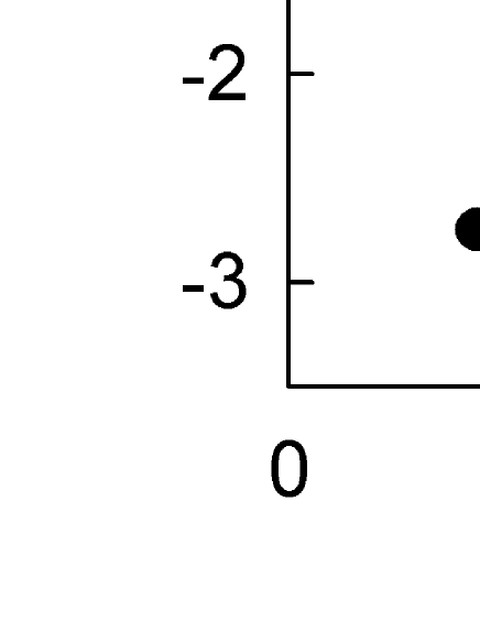
Figure 2: Same as Fig. 1 but the short-range part $\Delta V$ (65) is added to $V_{q\bar{q}}$ (63). $\alpha_{S}=0.234$ is obtained from a fit of the funnel potential on the ground state.

As our model only depends on ${\cal N}$, it is not able to reproduce the splittings between various potentials at short distances Juge2 . However, the constituent gluon picture can provide an intuitive explanation for this fine structure. Let us consider the ${\cal N}=0$ state. As ${\cal N}=2n_{y}+\ell_{y}$, the only possibility is $n_{y}=\ell_{y}=0$, which corresponds to the $\Pi_{u}$ state. For ${\cal N}=1$, we can only have $n_{y}=0$ and $\ell_{y}=1$. A possible mechanism to explain the short distance splitting of this state into three levels could be found in the relativistic corrections to the coulomb or the confining terms, that we neglected here. In particular, one of these corrections is a spin-orbit term proportional to $\bm{L}_{g}\cdot\bm{S}_{g}$ soon . Consequently, for a nonvanishing value of $\bm{L}_{g}$ (thus of $\ell_{y}$), and since the gluon is a spin $1$ particle, this spin-orbit term will split a level into three levels defined by their value of $\bm{J}_{g}=\bm{L}_{g}+\bm{S}_{g}$. Finally, for ${\cal N}=2$, a detailed lattice study reveals four levels Juge2 . We expect that one of them corresponds to $n_{y}=1$, $\ell_{y}=0$, and that the three others are $n_{y}=0$, $\ell_{y}=1$ states with the spin-orbit interaction separating them. To check this point, we need to include the spin structure of the gluon into the computation of the effective potential. This cannot be done analytically, and it is leaved for future works.

VII Conclusions

In this work, we studied two different pictures of hybrid mesons, which are both based on a spinless Salpeter Hamiltonian with a linear confinement. In particular, we applied the auxiliary fields technique to obtain analytical mass formula and wave functions of our models.

The first framework describing a hybrid meson is the excited flux tube. It relies on the idea that the flux tube (a Nambu-Goto string) linking the quark and the antiquark is not in its ground state, but in an excited one due to possible quantum fluctuations of the string. The excited string approach has been widely discussed in the literature (see for example Refs. Allen:1998wp ; luscher ). In particular, it can be shown that the interquark confining potential in this approach is of the form $V(r)=\sqrt{a^{2}r^{2}+2\pi aN+{\cal E}^{2}}$. Fundamental string theory states that ${\cal E}^{2}=-\pi a/6$ to preserve the Lorentz invariance at the quantum level. However, we argued in this study that since we are dealing with an effective string theory, we should rather look at the physical content of ${\cal E}^{2}$. As it can be interpreted as the square zero point energy of the string fluctuations, we proposed to consider ${\cal E}$ as the square zero point energy of the gluonic field, which is simulated in a simplified way by the string. Consequently, we are led to the conclusion that the usual value of ${\cal E}^{2}$ is not the best one for our purpose.

A second picture assimilates the hybrid meson to a three-body quark-antiquark-gluon bound state. The constituent gluon is then linked to the quark and the antiquark by two fundamental strings horn ; hyb1 . Thanks to the auxiliary fields technique, we have been able to find an analytic expression for this three-body system in the case of heavy and light hybrid mesons. In this last case, we found for the mass scale of the lightest hybrid mesons a value close to $2$ GeV. This is in agreement with other effective models llanes ; merlin and with lattice QCD computations Bern97 .

An interesting question is: how could the constituent gluon approach be reduced to a two-body model (only the quark and the antiquark) with an effective potential simulating the effect of the constituent gluon? In the heavy hybrid meson sector, we showed that the effective potential has the form of the excited flux tube interaction, with the gluon quantum numbers $(2n_{g}+\ell_{g})$ corresponding to the string excitation number $\mathcal{N}$. Moreover, the zero point energy of the excited flux tube, denoted as ${\cal E}$, is equal to the zero point energy of the heavy $q\bar{q}g$ system, when the $q\bar{q}$ energy is subtracted. Consequently, the constituent gluon picture is in this case equivalent to an effective string theory. In the light hybrid meson sector, the effective potential crucially depends on the quark-antiquark state, and only an asymptotic expression can be derived. This asymptotic expression is similar to the Lüscher term, but is now state dependent. It becomes universal only for highly excited quark-antiquark states.

Finally, we compared our results with lattice QCD predictions concerning the gluonic field energy levels Juge ; Juge2 . We find a good general agreement, but our model fails to describe the fine structure appearing at short distances. We argued that it was due to the fact that we did not take into account the gluon spin. Indeed, we showed by intuitive arguments that the spin-orbit interaction of the gluon should be able to roughly explain this fine structure, at least for the first excited states. The inclusion of the spin structure of the $q\bar{q}g$ system is thus a very interesting problem, which requires further investigations. Such a work is in progress.

- (1) K. J. Juge, J. Kuti, and C. J. Morningstar, Nucl. Phys. Proc. Suppl. 63, 326 (1998) [hep-lat/9709131]; K. J. Juge, J. Kuti, and C. Morningstar, Nucl. Phys. Proc. Suppl. 119, 682 (2003) [hep-lat/0209109].
- (2) K. J. Juge, J. Kuti, and C. Morningstar, Phys. Rev. Lett. 90, 161601 (2003) [hep-lat/0207004].
- (3) C. Mc Neile, Nucl. Phys. A 711, 303 (2002) [hep-lat/0207001], and references therein.
- (4) Y. Liu and X.-Q. Luo, Phys. Rev. D 73, 054510 (2006) [hep-lat/0511015], and references therein.
- (5) G. S. Adams et al., Phys. Rev. Lett. 81, 5760 (1998); S. U. Chung et al., Phys. Rev. D 65, 072001 (2002).
- (6) M. Lu et al., Phys. Rev. Lett 94, 032002 (2005) [hep-ex/0405044].
- (7) B. Aubert et al. [BABAR Collaboration], Phys. Rev. Lett. 95, 142001 (2005) [hep-ex/0506081].
- (8) F. E. Close and P. R. Page, Phys. Lett. B 628, 215 (2005) [hep-ph/0507199]; E. Klempt, hep-ph/0404270.
- (9) N. Isgur and J. Paton, Phys. Lett. B 124, 247 (1983); F. E. Close and P. R. Page, Nucl. Phys. 433, 233 (1995).
- (10) D. Horn and J. Mandula, Phys. Rev. D 17, 898 (1978).
- (11) A. Le Yaouanc, L. Oliver, O. Pène, J.-C. Raynal, and S. Ono, Z. Phys. C 28, 309 (1985); Yu. S. Kalashnikova, Z. Phys. C 62, 323 (1994).
- (12) T. Barnes and F. E. Close, Phys. Lett. B 116, 365 (1982).
- (13) D. LaCourse and M. G. Olsson, Phys. Rev. D 39, 2751 (1989).
- (14) T. J. Allen, M. G. Olsson, and S. Veseli, Phys. Lett. B 434, 110 (1998) [hep-ph/9804452].
- (15) M. Lüscher, K. Symanzik, and P. Weisz, Nucl. Phys. B 173, 365 (1980).
- (16) Yu. S. Kalashnikova and D. S. Kuzmenko, Phys. Atom. Nucl. 66, 955 (2003); Yad. Fiz. 66, 988 (2003) [hep-ph/0203128].
- (17) F. Buisseret and V. Mathieu, Eur. Phys. J. A 29, 343 (2006) [hep-ph/0607083].
- (18) C. Semay, B. Silvestre-Brac, and I. M. Narodetskii, Phys. Rev. D 69, 014003 (2004) [hep-ph/0309256].
- (19) A. B. Kaidalov, Yu. A. Simonov, Phys. Lett. B 636, 101 (2006) [hep-ph/0512151]; Yu. A. Simonov, hep-ph/0603148.
- (20) F. Buisseret and C. Semay, Phys. Rev. D 70, 077501 (2004) [hep-ph/0406216].
- (21) W. Lucha and F. F. Schöberl, Phys. Rev. A 54, 3790 (1996) [hep-ph/9603429]; F. Buisseret and C. Semay, Phys. Rev. E 71, 026705 (2005) [hep-ph/0409033].
- (22) F. Buisseret and C. Semay, Phys. Rev. D 71, 034019 (2005) [hep-ph/0412361].
- (23) M. G. Olsson and S. Veseli, Phys. Rev. D 51, 3578 (1995).
- (24) V. Mathieu, C. Semay, and F. Brau, Eur. Phys. J. A 27, 225 (2006) [hep-ph/0511210]; E. Abreu and P. Bicudo, hep-ph/0508281.
- (25) A. Yu. Dubin, A. B. Kaidalov, and Yu. A. Simonov, Phys. Atom. Nucl. 56, 1745 (1993); Yad. Fiz. 56, 213 (1993) [hep-ph/9311344].
- (26) S. Godfrey and N. Isgur, Phys. Rev. D 32, 189 (1985).
- (27) J. F. Arvis, Phys. Lett. B 127, 106 (1983); M. Lüscher and P. Weisz, JHEP 0407, 014 (2004) [hep-th/0406205].
- (28) L. Brink and H. B. Nielsen, Phys. Lett. B 45, 332 (1973).
- (29) S. Deldar, Phys. Rev. D 62, 034509 (2000) [hep-lat/9911008]; G. S. Bali, Phys. Rev. D 62, 114503 (2000) [hep-lat/0006022]; C. Semay, Eur. Phys. J. A 22, 353 (2004) [hep-ph/0409105].
- (30) F. Buisseret and C. Semay, Phys. Rev. D 73, 114011 (2006) [hep-ph/0511270].
- (31) S. D. Glazek and A. P. Szczepaniak, Phys. Rev. D 67, 034019 (2003) [hep-ph/0204248].
- (32) F. Brau and C. Semay, Phys. Rev. D 58, 034015 (1998) [hep-ph/0412179].
- (33) L. P. Fulcher, Phys. Rev. D 50, 447 (1994).
- (34) F. J. Llanes-Estrada and S. R. Cotanch, Phys. Lett. B 504, 15 (2001) [hep-ph/0008337]; I. J. General, S. R. Cotanch, and F. J. Llanes-Estrada, hep-ph/0609115.
- (35) J. Merlin and J. Paton, Phys. Rev. D 35, 1668 (1987).
- (36) C. Bernard et al., Phys. Rev. D 56, 7039 (1997) [hep-lat/9707008]; Z.-H. Mei and X.-Q. Luo, Int. J. Mod. Phys. A 18, 5713 (2003) [hep-lat/0206012].
- (37) Yu. S. Kalashnikova and Yu. B. Yufryakov, Phys. Atom. Nucl. 60, 307 (1997); Yad. Fiz. 60N2, 374 (1997) [hep- ph/9510357].
- (38) S. K. Bose, A. Jabs, and H. J. W. Müller-Kirsten, Phys. Rev. D 13, 1489 (1976).
- (39) Yu. S. Kalashnikova and D. S. Kuzmenko, Phys. Atom. Nucl. 67, 538 (2004); Yad. Fiz. 67, 556 ( 2004) [hep-ph/0302070].