Improved analysis of moments of $F_{3}$ in neutrino-nucleon scattering using the Bernstein polynomial method

Abstract

We use recently calculated next-to-next-to-leading order (NNLO) anomalous dimension coefficients for the moments of the $x{F}_{3}$ structure function in ${\nu}N$ scattering, together with the corresponding three-loop Wilson coefficients, to obtain improved QCD predictions for both odd and even moments of $F_{3}$. To investigate the issue of renormalization scheme dependence, the Complete Renormalization Group Improvement (CORGI) approach is used, in which all dependence on renormalization and factorization scales is avoided by a complete resummation of RG-predictable scale logarithms. We also consider predictions using the method of effective charges, and compare with the standard ‘physical scale’ choice. The Bernstein polynomial method is used to construct experimental moments (from the $x{F}_{3}$ data of the CCFR collaboration) that are insensitive to the value of $xF_{3}$ in the region of $x$ which is inaccessible experimentally. Direct fits for $\Lambda_{\textrm{\tiny{$\overline{{\rm MS}}$}}}^{(5)}$ ($\alpha_{s}(M_{Z})$) are then performed. The CORGI fits including target mass corrections give a value $\alpha_{s}(M_{Z})={0.1189}^{+0.0019}_{-0.0019}$, consistent with the world average. The effective charge and physical scale fits give slightly smaller values, which are still consistent within the errors.

1 Introduction

The measurements of the CCFR collaboration provide a precise determination of the non-singlet deep inelastic scattering (DIS) structure functions of neutrinos and anti-neutrinos on nucleons, $xF_{3}(x,Q^{2})$ [1]. Recently the NuTev collaboration have also published measurements of $F_{2}(x,Q^{2})$ and $F_{3}(x,Q^{2})$ [2]. The $Q^{2}$-dependence of moments of structure functions can be predicted in perturbative QCD, and fits to the data can be used to infer $\Lambda_{\textrm{\tiny{$\overline{{\rm MS}}$}}}$ (or equivalently $\alpha_{s}(M_{Z})$). In doing this, the principal difficulty is that there are upper and lower limits on the experimentally accessible range of $x$ at low and high $Q^{2}$, respectively. The moments are potentially sensitive to this missing information, and this propagates into an additional level of uncertainty in the resultant prediction of $\Lambda_{\textrm{\tiny{$\overline{{\rm MS}}$}}}$.

An approach which has been applied in the past is to use Bernstein polynomials, which are peaked in a rather limited $x$-range, to construct linear combinations of moments which are insensitive to the missing $x$ regions [3, 4]. The analysis of Ref. [3] chose, as is customary, to work in the $\overline{{\rm MS}}$ scheme and set both renormalization and factorization scales to $Q$ (physical scale (PS) choice). This was extended in Ref. [5] to consider predictions for $F_{3}$ obtained in the ‘complete renormalization group improved’ (CORGI) approach [6] in which all dependence on the renormalization scale $\mu$ and the factorization scale $M$ is eliminated by an all-orders resummation of RG-predictable scale logarithms.

The analyses of Refs. [3, 4] and [5] used the then state-of-the-art three-loop (NNLO) results for the anomalous dimension and coefficient function, which were restricted to a subset of odd moments $n=1,3,5,\ldots,13$ [7]. Recent progress has yielded NNLO results for these quantities for any value of $n$ [8, 9]. Consequently the set of Bernstein moments used in the fits can now be greatly extended. The Bernstein polynomials defined in Refs. [3, 4] were linear combinations of odd moments, but the new results of Refs. [8, 9] mean that, by a slight redefinition of the polynomials, even moments can now also be studied.

In this paper we intend to perform such an extended analysis. We shall fit the CCFR data [1] to PS and CORGI NNLO QCD predictions, and will in addition compare with the predictions in the closely-related method of effective charges approach (EC) [10]. Target mass corrections and higher twist effects will also be considered. We shall also compare our results to those obtained using a fitting technique based on Jacobi Polynomials [11, 12, 13].

The plan of the paper is to give a brief review of the factorization and renormalization scheme dependence of structure function moments in Section 2. In Section 3 we discuss the CORGI and effective charge approaches for leptoproduction moments. We take this opportunity to correct an error in the expression for the NNLO CORGI result for the scheme invariant $X_{2}$ derived in Ref. [5]. Section 4 will contain a description of the Bernstein polynomial averages to be employed in the fits. We shall show how to modify the definition of the polynomials to accommodate both odd and even moments. We then constrain the set of acceptable Bernstein moments to be used in the fits by comparing how four different methods of extrapolation (to obtain $xF_{3}$ on the full $x$-range) differ; this enables us to define a ‘modelling error’ to be combined with the other sources of error in our analysis. In section 5 we give details of the fitting procedure and in section 6 we present the results of the fits to the PS, CORGI and EC predictions for the moments, and consider how the fits change if target mass corrections and higher twist corrections are included. Section 7 contains a discussion and conclusions.

2 Factorization and renormalization scheme dependence of the moments

The moments we are concerned with in this paper are those derived from $F_{3}$ in (anti)neutrino-nucleon scattering. They are defined as:

$${\cal M}_{3}^{\nu N}(n;Q^{2}) = \int_{0}^{1}dx\;x^{n-1}F_{3}^{\nu N}(x,Q^{2}).$$ (1)

These moments can be factorized in the following form,

$${\cal M}_{3}^{\nu N}(n;Q^{2}) = \langle N|{\cal O}_{n,\;\textrm{\tiny{NS}}}(M)|N\rangle\,{\cal C}^{(3)}_{n}(Q,M,\mu,a(\mu)),$$ (2)

where $\langle N|{\cal O}_{n,NS}(M)|N\rangle$ is the non-singlet (NS) operator matrix element of nucleon states and ${\cal C}^{(3)}_{n}(Q,M,\mu,a(\mu))$ is the coefficient function. Here $a\equiv{\alpha}_{s}/\pi$ is the RG-improved coupling. The operator matrix element is factorized at the scale $M$ into a non-perturbative component and a perturbative expression, written in terms of the coupling evaluated at the factorization scale, $a=a(M)$. The factorization scale dependence is governed by the anomalous dimension equation,

$$M\frac{\partial}{\partial M}\langle N|{\cal O}_{n,\;\textrm{\tiny{NS}}}(M)|N\rangle = \langle N|{\cal O}_{n,\;\textrm{\tiny{NS}}}(M)|N\rangle\gamma_{n,\;\textrm{\tiny{NS}}}(a).$$ (3)

Here ${\gamma}_{n,\;\textrm{\tiny{NS}}}(a)$ is the anomalous dimension of the moment. It has the following perturbative expansion,

$${\gamma}_{n,\;\textrm{\tiny{NS}}}(a) = -d(n)a-d_{1}(n)a^{2}-d_{2}(n)a^{3}-d_{3}(n)a^{4}-\ldots,$$ (4)

where $d(n)$ is factorization scheme invariant, and the higher coefficients serve to label the factorization scheme dependence. The $M$-dependence of the coupling is governed by the beta-function equation,

$$M\frac{\partial a}{\partial M} = {\beta}(a)\;\equiv\;-ba^{2}(1+ca+c_{2}a^{2}+c_{3}a^{3}+\ldots).$$ (5)

Here $b=(33-2{N}_{f})/6$ and $c=(153-19N_{f})/12b$ are renormalization scheme (RS) invariant. The higher coefficients serve to label the RS dependence. Together, these two equations determine the perturbative behaviour of the operator matrix element. For the remainder of this paper we simplify our notation by dropping the sub- and superscripts ‘$\nu N$’, ‘$n$’, ‘$(3)$’ and ‘NS’, from the quantities in Eqs. (2) and (3). Also, although the coefficients $d_{i}(n)$ in Eq. (4) are $n$-dependent, we also suppress this.

A solution to Eq. (3) can be obtained in the form,

$$\langle\mathcal{O}(M)\rangle = A_{n}\exp\left\{\int_{0}^{a(M)}\frac{\gamma(x)}{\beta(x)}dx-\int_{0}^{\infty}\frac{\gamma^{(1)}(x)}{\beta^{(2)}(x)}dx\right\},$$ (6)

where $\gamma^{(i)}$ and $\beta^{(i)}$ denote the anomalous dimension and beta-function equations truncated after $i$ terms. There is a distinct parallel between the above equation and the solution to the beta function equation. The second integral in Eq. (6) is an infinite constant. We are free to choose any form we wish for this term, subject to the constraint that it must have the same singularity structure as the first integral. However, a particular choice for this constant corresponds to a particular definition of $A_{n}$. Consequently, $A_{n}$ can be likened to the dimensional transmutation parameter, $\Lambda$, in that it defines the missing boundary condition in Eq. (3). $A_{n}$ is actually a (set of) non-perturbative constant(s), generated by the factorization process, and they are factorization and renormalization scheme (FRS) invariant. Their precise values cannot be calculated within perturbation theory, and hence must be obtained by comparison with experimental data.

The coefficient function ${\cal C}(Q,M,\mu,a(\mu))$, depends on both the renormalization and factorization scheme adopted, and it takes the form of an expansion in powers of the coupling evaluated at the renormalization scale,

$${\cal C}(Q,M,\mu,{\tilde{a}}(\mu)) = 1+r_{1}\tilde{a}+r_{2}\tilde{a}^{2}+r_{3}\tilde{a}^{3}+\ldots,$$ (7)

where $\tilde{a}=a(M=\mu)$. Using the above equation together with Eqs. (2) and (6), the moments can be written as [5, 15, 16],

$${\cal M}(n;Q^{2}) = A_{n}\left(\frac{ca}{1+ca}\right)^{d/b}\exp(\mathcal{I}(a))(1+r_{1}\tilde{a}+r_{2}\tilde{a}^{2}+r_{3}\tilde{a}^{3}+\cdots),$$ (8)

where,

$${\cal I}(a) = \int_{0}^{a}dx\frac{d_{1}+(d_{1}c+d_{2}-dc_{2})x+(d_{3}+cd_{2}-c_{3}d)x^{2}+\cdots)}{b(1+cx)(1+cx+c_{2}x^{2}+c_{3}x^{3}+\cdots)}.$$ (9)

The explicit $M$ dependence of the coupling can be obtained by solving the following transcendental equation [14],

$$\frac{1}{a}+c\ln\frac{ca}{1+ca} = b\ln\frac{M}{\tilde{\Lambda}}-b\int_{0}^{a}\left[\frac{1}{\beta(x)}-\frac{1}{\beta^{(2)}(x)}\right].$$ (10)

Equation (8) serves as a prototypical expression for the moments, from which CORGI, EC and PS predictions can be derived.

The self-consistency of perturbation theory means that the perturbative coefficient $r_{1}$ has a dependence on $M$ and $d_{1}$. The higher coefficients also have a dependence on the parameters specifying the FRS, ${r_{k}}({\mu},M,{c_{2}},c_{3},{\ldots},{c_{k}};{d_{1}},{d_{2}},{\ldots},{d_{k}})$. The explicit form of this FRS-dependence can be determined by demanding that on calculating the moments up to O($a^{k}$) the partial derivative with respect to each FRS parameter is O($a^{k+1}$) [15, 16] . The complete set of partial derivatives required to derive the FRS-dependence of $r_{1}$, $r_{2}$ and $r_{3}$ is, for the $\mu$-dependence

$$\mu\frac{\partial r_{1}}{\partial\mu}\;=\;0,\qquad\mu\frac{\partial r_{2}}{\partial\mu}\;=\;r_{1}b,\qquad\mu\frac{\partial r_{3}}{\partial\mu}\;=\;2r_{2}b+br_{1}c.$$ (11)

For the $M$-dependence we have

$$M\frac{\partial r_{1}}{\partial M}\;=\;d,\qquad M\frac{\partial r_{2}}{\partial M}\;=\;dr_{1}-dL+d_{1},$$

$$M\frac{\partial r_{3}}{\partial M}\;=\;d_{2}+d_{1}r_{1}+dr_{2}-dr_{1}L-2d_{1}L+dL^{2}-dcL,$$ (12)

where we have defined $L\equiv b{\ln}(M/\mu)$. For the $c_{2}$-dependence we have

$$\frac{\partial r_{1}}{\partial c_{2}}\;=\;0,\qquad\frac{\partial r_{2}}{\partial c_{2}}\;=\;-\frac{d}{2b},$$

$$\frac{\partial r_{3}}{\partial c_{2}}\;=\;-\frac{r_{1}d}{2b}+\frac{Ld}{b}+\frac{cd}{3b}-\frac{2d_{1}}{3b}-r_{1}.$$ (13)

For the $c_{3}$-dependence

$$\frac{\partial r_{1}}{\partial c_{3}}\;=\;0,\qquad\frac{\partial r_{2}}{\partial c_{3}}\;=\;0,\qquad\frac{\partial r_{3}}{\partial c_{3}}\;=\;-\frac{d}{6b}.$$ (14)

For the $d_{1}$-dependence

$$\frac{\partial r_{1}}{\partial d_{1}}\;=\;-\frac{1}{b},\qquad\frac{\partial r_{2}}{\partial d_{1}}\;=\;\frac{c}{2b}-\frac{r_{1}}{b}+\frac{L}{b},$$

$$\frac{\partial r_{3}}{\partial d_{1}}\;=\;\frac{cr_{1}}{2b}-\frac{c^{2}}{3b}-\frac{r_{2}}{b}+\frac{c_{2}}{3b}-\frac{L^{2}}{b}+\frac{Lr_{1}}{b}.$$ (15)

For the $d_{2}$-dependence we have

$$\frac{\partial r_{1}}{\partial d_{2}}\;=\;0,\qquad\frac{\partial r_{2}}{\partial d_{2}}\;=\;-\frac{1}{2b},\qquad\frac{\partial r_{3}}{\partial d_{2}}\;=\;\frac{c}{3b}+\frac{1}{2b}(2L-r_{1}).$$ (16)

Finally, for the $d_{3}$-dependence we have

$$\frac{\partial{r}_{1}}{\partial{d_{3}}}\;=\;0,\qquad\frac{\partial{r_{2}}}{\partial{d_{3}}}\;=\;0,\qquad\frac{\partial r_{3}}{\partial d_{3}}\;=\;-\frac{1}{3b}.$$ (17)

These results may now be integrated to obtain $r_{1}$, $r_{2}$ and $r_{3}$. For $r_{1}$ we obtain

$$r_{1} = \frac{d}{b}\tau_{M}-\frac{d_{1}}{b}-X_{0}(Q),$$ (18)

where $\tau_{M}=b\ln\left(M/\tilde{\Lambda}\right)$. $X_{0}(Q)$ is an FRS invariant quantity, generated as a constant of integration. One can define an FRS invariant, non-universal scale parameter, $\Lambda_{{\cal M}}$, via the FRS invariant $X_{0}(Q)$. Thus,

$$\frac{d}{b}\tau_{M}-\frac{d_{1}}{b}-r_{1} = X_{0}(Q)\;\equiv\;d\;\ln\left(\frac{Q}{\Lambda_{{\cal M}}}\right).$$ (19)

For $r_{2}$ we obtain

$$r_{2} = \Bigg{(}\frac{1}{2}-\frac{b}{2d}\Bigg{)}r_{1}^{2}+\frac{b}{d}r_{1}\tilde{r}_{1}+\frac{d_{1}}{d}r_{1}-\frac{dc_{2}}{2b}+\frac{d_{1}^{2}}{2bd}+\frac{cd_{1}}{2b}-\frac{d_{2}}{2b}+X_{2},$$ (20)

where we have defined,

$$\tilde{r}_{1} \equiv r_{1}(M=\mu)$$ (21)

$$= \frac{d}{b}\tau_{\mu}-\frac{d_{1}}{b}-X_{0}(Q).$$

Here $X_{2}$ is another FRS-invariant constant of integration. Crucially $X_{2}$ and higher invariants are independent of $Q$. Hence, the complete $Q$-dependence of the observable is generated by $X_{0}(Q)$. Similarly, for $r_{3}$ we obtain

$$r_{3} = \frac{c_{2}dc}{3b}-\frac{c_{3}d}{6b}+\frac{cd_{2}}{3b}-\frac{d_{3}}{3b}-\frac{2d_{1}^{3}}{3bd^{2}}-\frac{cd_{1}^{2}}{2bd}-\frac{c^{2}d_{1}}{3b}+\frac{d_{1}d_{2}}{bd}+\frac{c_{2}d_{1}}{3b}$$ (22)

$$- \frac{2d_{1}^{2}r_{1}}{d^{2}}-\frac{d_{1}r_{1}^{2}}{d}+\frac{b^{2}r_{1}^{3}}{3d^{2}}-\frac{r_{1}^{3}}{3}-\frac{bcr_{1}^{2}}{2d}+\frac{d_{2}r_{1}}{d}$$

$$- \frac{2bd_{1}r_{1}\tilde{r}_{1}}{d^{2}}-\frac{b^{2}r_{1}\tilde{r}_{1}^{2}}{d^{2}}-\frac{br_{1}^{2}\tilde{r}_{1}}{d}+\frac{bcr_{1}\tilde{r}_{1}}{d}$$

$$+ \frac{2b\tilde{r}_{1}r_{2}}{d}+\frac{2d_{1}r_{2}}{d}+r_{1}r_{2}+X_{3}.$$

Again $X_{3}$ is a $Q$-independent FRS-invariant constant of integration. Using Eq. (20) $X_{3}$ can be written in terms of $r_{1}$, ${\tilde{r}}_{1}$ and the other FRS parameters. This also holds for the higher invariants. The results of Eqs. (11) - (17) and of Eqs. (20) and (22) replace, respectively, Eqs. (15) and (18) of Ref. [5] which contain several errors. The invariant $X_{2}$ can be obtained from NNLO results for the anomalous dimension coefficients and coefficient function in any FRS. For instance if we make the customary choice of $\overline{{\rm MS}}$ with $M=\mu=Q$ then $r_{1}={\tilde{r_{1}}}$ and we obtain

$$X_{2} = \left.r_{2}-\Bigg{(}\frac{1}{2}+\frac{b}{2d}\Bigg{)}r_{1}^{2}-\frac{d_{1}}{d}r_{1}+\frac{dc_{2}}{2b}-\frac{d_{1}^{2}}{2bd}-\frac{cd_{1}}{2b}+\frac{d_{2}}{2b}\right|_{\overline{{\rm MS}}}.$$ (23)

In summary, through Eqs. (18), (20) and (22), we have determined the explicit FRS dependence of the coefficients $r_{i}$. In doing so, we have generated a set of FRS invariant quantities $X_{i}$, the importance of which will become clear when we come to consider the CORGI form of the moments in the following section.

3 PS, CORGI and EC predictions

The standard physical scale approach is to set $M=\mu=Q$ and adopt $\overline{{\rm MS}}$ subtraction. Setting $M=\mu$ implies that $a=\tilde{a}$, and hence the moments have the form,

$${\cal M}(n;Q^{2}) = A_{n}\left(\frac{ca}{1+ca}\right)^{d/b}\left(1+R_{1}a+R_{2}a^{2}+\ldots\right).$$ (24)

The coefficients $R_{i}$ can be determined by expanding Eq. (8) in powers of $a$,

$$R_{1} = r_{1}+\frac{d_{1}}{b}$$ (25)

$$R_{2} = r_{2}+\frac{d_{1}^{2}}{2b^{2}}-\frac{cd_{1}}{2b}+\frac{r_{1}d_{1}}{b}-\frac{dc_{2}}{2b}+\frac{d_{2}}{2b},$$ (26)

and the coupling in this expression is the three-loop $\overline{{\rm MS}}$ coupling with $\mu=Q$.

The CORGI idea (see Ref. [6] for a detailed discussion) is that all RG-predictable information about higher perturbative coefficients, available at a given fixed-order of calculation should be resummed to all-orders. Given an NLO calculation for instance one knows $X_{0}(Q)$ but not $X_{2},\;X_{3}$ or higher FRS-invariants. One should therefore resum to all-orders all the terms not involving these unknown invariants. As discussed in Section 2 these terms are multinomials in $r_{1},{\tilde{r}_{1}},c_{2},\ldots,c_{i},d_{1},d_{2},\ldots,d_{i},\ldots$.

Crucially this all-orders sum must be FRS-invariant, as separately must be the subset of terms involving $X_{2}$, $X_{3}\ldots$. One may exploit this invariance and choose to use the FRS where all the FRS parameters are zero, ${r_{1}}={\tilde{r}_{1}}=c_{2}=\ldots={c}_{i}=\ldots=d_{1}=d_{2}=\ldots={d}_{i}=\ldots=0$.

Setting $r_{1}={\tilde{r}_{1}}=0$ means that $\mu=M$, setting $d_{1}=0$ then implies that (from Eq. (19)) ${\tau}_{M}=b{\ln}(Q/{\Lambda}_{{\cal M}})$. Also, with $c_{i}={d}_{i}=0$ the integral ${\cal I}(a)$ of Eq. (9) vanishes, and one finally obtains the CORGI form of the moments,

$${\cal M}(n;Q^{2}) = A_{n}\left(\frac{ca_{0}}{1+ca_{0}}\right)^{d/b}\left(1+X_{2}a_{0}^{2}+X_{3}a_{0}^{3}+\ldots\right).$$ (27)

Here the CORGI coupling $a_{0}$ is the coupling in a ’t Hooft scheme [17], in which $c_{i}=0$ $(i>1)$. This can be written in terms of the Lambert $W$ function defined implicitly by $W(z){e}^{W(z)}=z$ [18, 19],

$$a_{0}(Q) = \frac{-1}{c\left[1+W_{-1}(z(Q))\right]},$$ (28)

with,

$$z(Q) = -\frac{1}{{\rm e}}\left(\frac{Q}{{\Lambda}_{{\cal M}}}\right)^{-b/c}.$$ (29)

$W_{-1}$ refers to the branch of the Lambert $W$ function required for asymptotic freedom, the nomenclature being that of Ref. [20]. $\Lambda_{{\cal M}}$ is the invariant scale connected with the $X_{0}(Q)$ FRS-invariant, defined in Eq. (19). Since it is an FRS-invariant it can be evaluated in any FRS. Choosing the $\overline{{\rm MS}}$ scheme with $M=\mu=Q$ one finds

$$\Lambda_{{\cal M}} = \Lambda_{\textrm{\tiny{$\overline{{\rm MS}}$}}}{\left(\frac{2c}{b}\right)}^{-c/b}\exp\left\{\frac{d_{1}}{db}+\frac{r_{1}}{d}\right\},$$ (30)

with $r_{1}$ and $d_{1}$ calculated in $\overline{{\rm MS}}$ with $M=\mu=Q$. The factor of ${\left(\frac{2c}{b}\right)}^{-c/b}$ converts to the standard convention for integrating the beta-function equation and defining $\Lambda_{\textrm{\tiny{$\overline{{\rm MS}}$}}}$ (see Ref. [21] for further details). The second factor on the r.h.s. of Eq. (27) resums to all-orders the RG-predictable terms not involving $X_{2},X_{3},\ldots$. The $a_{0}^{2}$ term sums to all-orders the RG-predictable terms involving $X_{2}$, but not $X_{3},X_{4},\ldots$, etc.

The CORGI result corresponds to an $\overline{{\rm MS}}$ scale choice $M=\mu=xQ$, with

$$x = x_{\textrm{\tiny{CORGI}}}\;\equiv\;\exp\left\{-\frac{d_{1}}{db}-\frac{r_{1}}{d}\right\}.$$ (31)

To illustrate how the CORGI scale differs from the PS choice ($x=1$) we plot in table 1 the $x_{\textrm{\tiny{CORGI}}}$, for the first $20$ moments $n=1,2,\ldots,20$. We also tabulate the corresponding $X_{2}(n)$ NNLO CORGI invariants obtained from Eq. (23). The anomalous dimension coefficients up to NNLO are taken from Refs. [8, 9], and the coefficient function from Ref. [7]. We assume $N_{f}=5$ active quark flavours.

$n$	$x_{\textrm{\tiny{CORGI}}}$		$X_{2}(n)$
1	0.4688		-1
2	0.7156		-3.01
3	0.5074		-3.28
4	0.42966		-3.485
5	0.3838		-3.627
6	0.3530		-3.713
7	0.3300		-3.766
8	0.312		-3.792
9	0.2974		-3.8
10	0.2853		-3.793

$n$	$x_{\textrm{\tiny{CORGI}}}$		$X_{2}(n)$
11	0.2749		-3.776
12	0.2659		-3.749
13	0.2580		-3.716
14	0.2510		-3.677
15	0.2447		-3.633
16	0.2390		-3.586
17	0.2338		-3.536
18	0.2291		-3.483
19	0.2248		-3.428
20	0.2207		-3.372

Table 1: The numerical values of $x_{\textrm{\tiny{CORGI}}}$ and the NNLO CORGI invariants ${X}_{2}(n)$ for the $n=1-20$ moments of $F_{3}$.

We see from table 1 that as $n$ increases the CORGI scale decreases, becoming significantly less than $x=1$ (PS). The $X_{2}(n)$ invariants are seen to be moderate in size.

Finally, we discuss the third variant of perturbative QCD which we shall consider. By setting $M=\mu$ and rearranging, we can recast the perturbation series for ${\cal M}(n;Q^{2})$ of Eq. (8) in the form

$${\cal M}(n;Q^{2}) = A_{n}\left(c\tilde{R}(a)\right)^{d/b},$$ (32)

where

$$\tilde{R}(a) = a+\tilde{R}_{1}a^{2}+\tilde{R}_{2}a^{3},$$ (33)

is an effective charge [10], and the coefficients $\tilde{R}_{i}$ have the form,

$$\tilde{R}_{1} = \frac{bcR_{1}}{d}-c^{2}$$ (34)

$$= \frac{bcr_{1}}{d}+\frac{d_{1}c}{d}-c^{2},$$

$$\tilde{R}_{2} = \frac{bcR_{2}}{d}+\frac{b^{2}R^{2}_{1}c}{2d^{2}}-\frac{bR_{1}^{2}c}{2d}-\frac{bR_{1}c^{2}}{d}+c^{3}$$ (35)

$$= \frac{bcr_{2}}{d}+\frac{bd_{1}r_{1}c}{d^{2}}+\frac{d_{2}c}{2d}-\frac{c_{2}c}{2}$$

$$+ \frac{b^{2}r^{2}_{1}c}{2d^{2}}-\frac{br_{1}^{2}c}{2d}+\frac{d_{1}^{2}c}{2d^{2}}-\frac{br_{1}c^{2}}{d}-\frac{3d_{1}c^{2}}{2d}+c^{3}.$$

Here $R_{1}$ and $R_{2}$ are the coefficients defined in Eqs. (25) and (26). Rather than integrating the effective charge beta-function we shall instead apply CORGI to the effective charge, avoiding the need to numerically solve a transcendental equation which would make the fitting to data considerably more complicated. At NLO the CORGI and EC results agree exactly. We have the CORGI result

$${\cal M}(n;Q^{2}) = A_{n}c^{d/b}\left(a_{0}+\tilde{X}_{2}a_{0}^{3}+\tilde{X}_{3}a_{0}^{4}+\ldots\right)^{d/b}.$$ (36)

In this case, the $\tilde{X}_{i}$ coefficients are the CORGI invariants corresponding to single scale RS-dependence [6]. They have the form,

$$\tilde{X}_{2} = \tilde{R}_{2}-\tilde{R}_{1}^{2}-c\tilde{R}_{1}+c_{2},$$ (37)

$$\tilde{X}_{3} = \tilde{R}_{3}-3\tilde{R}_{1}\tilde{R}_{2}+2\tilde{R}_{1}^{3}+\frac{c\tilde{R}_{1}^{2}}{2}-\tilde{R}_{1}c_{2}+\frac{1}{2}c_{3}.$$ (38)

The CORGI coupling $a_{0}$ is that of Eq. (28) but with the scale $\Lambda_{{\cal M}}$ now defined by,

$$\Lambda_{{\cal M}}^{\textrm{\tiny{EC}}} = \left(\frac{2c}{b}\right)^{-c/b}\exp\left(\frac{\tilde{R}_{1}}{b}\right)\Lambda_{\textrm{\tiny{$\overline{{\rm MS}}$}}}.$$ (39)

We shall refer to this variant of perturbation theory as ‘EC’ for simplicity, even though as noted above it is really CORGI applied to a single-scale effective charge.

We note that we can streamline the calculation of the FRS-invariants $X_{i}$ by using the single-scale effective charge. If we set $M=\mu$ in Eq. (8), then the moments reduce to a single-scale problem [6]. We can then rearrange the resultant expression in terms of an effective charge, $\hat{R}(a)$,

$${\cal M}(n;Q^{2}) = A_{n}\left(\frac{c\hat{R}(a)}{1+c\hat{R}(a)}\right)^{d/b}.$$ (40)

$\hat{R}(a)$ has the form,

$$\hat{R}(a) = a+\hat{R}_{1}a^{2}+\hat{R}_{2}a^{3}+\hat{R}_{3}a^{4}+\ldots.$$ (41)

The coefficients $\hat{R}_{i}$ can be determined by expanding Eqs. (24) and (40) in powers of $a$ and then equating coefficients. They are found to be,

$$\hat{R}_{1} = \frac{b}{d}R_{1},$$ (42)

$$\hat{R}_{2} = \frac{b}{d}\left(R_{2}+cR_{1}-\frac{R_{1}^{2}}{2}+\frac{bR_{1}^{2}}{2d}\right),$$ (43)

where $R_{1}$ and $R_{2}$ are given by Eqs. (25) and (26). If we then CORGI-ize this effective charge, we have a new set of FRS invariants [6],

$$\hat{X}_{0} = b\ln\frac{M}{\tilde{\Lambda}}-\hat{R}_{1},$$ (44)

$$\hat{X}_{2} = \hat{R}_{2}-\hat{R}_{1}^{2}-c\hat{R}_{1}+c_{2},$$ (45)

and the moments become,

$${\cal M}(n;Q^{2}) = A_{n}\left(\frac{c\left(a_{0}+\hat{X}_{2}a_{0}^{3}\right)}{1+c\left(a_{0}+\hat{X}_{2}a_{0}^{3}\right)}\right)^{d/b}.$$ (46)

Expanding this into a form which we can compare with Eq. (27), gives,

$${\cal M}(n;Q^{2}) = A_{n}\left(\frac{ca_{0}}{1+ca_{0}}\right)^{d/b}\left(1+\frac{d}{b}\hat{X}_{2}\,a_{0}^{2}+\ldots\right).$$ (47)

Isolating the ${\cal O}(a_{0}^{2})$ in the RHS bracket of the above equation, and then using Eqs. (45), (42), (43), (25) and (26), gives,

$$\frac{d}{b}\hat{X}_{2} = \frac{d}{b}\left(\hat{R}_{2}-\hat{R}_{1}^{2}-c\hat{R}_{1}+c_{2}\right)$$ (48)

$$= r_{2}-\Bigg{(}\frac{1}{2}+\frac{b}{2d}\Bigg{)}r_{1}^{2}-\frac{d_{1}}{d}r_{1}+\frac{dc_{2}}{2b}-\frac{d_{1}^{2}}{2bd}-\frac{cd_{1}}{2b}+\frac{d_{2}}{2b}.$$ (49)

So we see that the coefficient of the ${\cal O}(a^{2})$ term in Eq. (47) is the FRS invariant $X_{2}$, of Eq. (23) with $\mu=M$ ($r_{1}=\tilde{r}_{1}$). Isolating the $a^{3}$ term will yield $X_{3}$, and so on for higher $X_{i}$.

The coupling in Eq. (47) is the ’t Hooft coupling of Eq. (28), but with the scale parameter determined by Eq. (44). Evaluating Eq. (44) in $\overline{{\rm MS}}$ with $M=\mu=Q$ and using the standard definition of the single-scale RS invariant $\hat{X}_{0}$ [10, 14] gives,

$$\hat{X}_{0}(Q) \equiv b\ln\frac{Q}{{\Lambda}_{{\cal M}}}$$ (50)

$$= b\ln\frac{Q}{\tilde{\Lambda}}-\hat{R}_{1}.$$ (51)

Comparison with Eq. (19) then reveals that $\hat{X}_{0}(Q)=(b/d)X_{0}(Q)$. Using the same procedure we can obtain expressions for $X_{3}$ and higher CORGI invariants.

Non-perturbative effects

The three variants of NNLO perturbative QCD, PS, CORGI, and EC, can all be computed given $\overline{{\rm MS}}$ anomalous dimension coefficients up to NNLO [8, 9], and the coefficient function [7]. However, these perturbative predictions will be subject to non-perturbative corrections in the form of ${\cal O}\left(1/Q^{2}\right)$ terms. The two principal sources of these terms are: higher twist terms and effects due to the mass of the target hadron.

The perturbative form of the moments is derived under the assumption that the mass of the target hadron is zero (in the limit $Q^{2}\rightarrow\infty$). At intermediate and low $Q^{2}$ this assumption will begin to break down and the moments will be subject to potentially significant power corrections, of order ${\cal O}\left(m_{N}^{2}/Q^{2}\right)$, where $m_{N}$ is the mass of the nucleon. These are known as target mass corrections (TMCs) and when included, the $F_{3}$ moments have the form [22, 23],

$${\cal M}^{\textrm{\tiny{TMC}}}(n;Q^{2}) = {\cal M}(n;Q^{2})+\frac{n(n+1)}{n+2}\frac{m_{N}^{2}}{Q^{2}}{\cal M}(n+2;Q^{2})+{\cal O}\left(\frac{m_{N}^{4}}{Q^{4}}\right).$$ (52)

The moments will also be subject to corrections from sub-leading twist contributions to the OPE. These effects are poorly understood and hence we only estimate them; this is done by means of an unknown parameter, $A_{\textrm{\tiny{HT}}}$. The estimate has the form [3],

$${\cal M}^{\textrm{\tiny{HT}}}(n;Q^{2}) = n\left(A^{\textrm{\tiny{HT}}}\frac{\Lambda_{\textrm{\tiny{$\overline{{\rm MS}}$}}}^{2}}{Q^{2}}\right){\cal M}(n;Q^{2}),$$ (53)

and the value of $A^{\textrm{\tiny{HT}}}$ is obtained by fitting to data. Due to the poorly understood nature of these effects, we do not include the above term in the full analysis. Rather, we perform the analysis with and without this term included, and take the difference in the results as an estimate of the error associated with our ignorance of the true nature of these effects.

The bottom quark mass threshold is within the range of $Q^{2}$ spanned by the available data for $F_{3}$. It is therefore necessary to evolve the expressions for the moments over this threshold, and in order to do this we use the formalism of Ref. [25]. We use massless QCD with 4 quarks for $Q^{2}\leq m_{b}^{2}$ and massless QCD with 5 quarks for $Q^{2}>m_{b}^{2}$. Here $m_{b}$ is the pole mass of the $b$-quark with ${m}_{b}=4.85\pm{0.15}$ MeV [24]. From the decoupling theorem, one finds the following relation between the coupling above and below a quark threshold (denoted by $a_{f+1}(Q^{2})$ and $a_{f}(Q^{2})$ respectively) [25]

$$a_{f}(m_{b}^{2}) = a_{f+1}(m_{b}^{2})+\frac{11}{72}\left(a_{f+1}(m_{b}^{2})\right)^{3}.$$ (54)

In practice, this matching is implemented by adopting different values of the scale parameter in different $N_{f}$ regions. This is governed by the following equations [25],

$${\Lambda}_{N_{f}+1}^{2} = {\Lambda}_{N_{f}}^{2}\left(\frac{m_{N_{f}+1}^{2}}{{\Lambda}_{N_{f}}^{2}}\right)^{1-\frac{b^{N_{f}}}{b^{N_{f}+1}}}\times\exp\left(\frac{\delta_{\textrm{\tiny{NLO}}}+\delta_{\textrm{\tiny{NNLO}}}}{2b^{N_{f}+1}}\right),$$ (55)

where $\delta_{\textrm{\tiny{NLO}}}$ and $\delta_{\textrm{\tiny{NNLO}}}$ are given by

$$\delta_{\textrm{\tiny{NLO}}} = 4(c^{N_{f}+1}-c^{N_{f}})\ln L_{m}-4c^{N_{f}+1}\ln\frac{b^{N_{f}+1}}{b^{N_{f}}},$$ (56)

$$\delta_{\textrm{\tiny{NNLO}}} = \frac{8}{b^{N_{f}}L_{m}}\left(\left(c^{N_{f}+1}-c^{n_{f}}\right)c^{N_{f}}\ln L_{m}+\left(c^{N_{f}+1}\right)^{2}-\left(c^{N_{f}}\right)^{2}\right.$$ (57)

$$+ \left.c_{2}^{N_{f}}-c_{2}^{N_{f}+1}+\frac{7}{384}\right).$$

Here, ${\Lambda}_{N_{f}}$ is the scale parameter in the region where $N_{f}$ quarks are active, $m_{N_{f}}$ is the pole mass of the $f$ quark, $b^{N_{f}}$, $c^{N_{f}}$ and $c_{2}^{N_{f}}$ are simply $b$, $c$ and $c_{2}$ evaluated for $N_{f}$ quark flavours and we have defined $L_{m}\equiv\ln\left(m_{N_{f}+1}^{2}/{\Lambda}_{N_{f}}^{2}\right)$. Furthermore, we also demand continuity of the moments at the threshold i.e.

$$\left.{\cal M}(n;m_{b}^{2})\right|_{N_{f}=4} = \left.{\cal M}(n;m_{b}^{2})\right|_{N_{f}=5}.$$ (58)

As a consequence of this, the parameters $A_{n}$ also have different values in the $N_{f}=4$ and $N_{f}=5$ regions and their values are related by,

$$A_{n}^{(5)} = \left(\left.\frac{A_{n}}{{\cal M}(n;m_{b}^{2})}\right|_{N_{f}=5}\,\right)\left(\left.\frac{{\cal M}(n;m_{b}^{2})}{A_{n}}\right|_{N_{f}=4}\,\right)A_{n}^{N_{f}=4}.$$ (59)

4 The method of Bernstein averages

Figure 1: Data for $xF_{3}$ plotted against $x$ for the 12 different $Q^{2}$ bins of the CCFR data.

When comparing theoretical predictions for moments of structure functions with experimental data, we are faced with the long-standing issue of missing data regions at high and low $x$ for low and high $Q^{2}$ respectively. This is demonstrated in Fig. 1 in which we plot the CCFR data [1] for 12 different values of $Q^{2}$. We can see that at the lower range of $Q^{2}$ we are limited to low-$x$ data, and that at high $Q^{2}$ we are limited to the high $x$ range.

In order to reliably evaluate a moment at a particular $Q^{2}$, we require data for the whole range of $x$. This being unavailable, we are forced to make some guess about how the structure function behaves in the missing data region. That is to say, we have to choose some method of modelling (extrapolating and interpolating) the data to cover the full range of $x$. However we wish to make the evaluation of the experimental moments as free from QCD input as possible, thus making the comparison between theory and experiment as direct as possible. To this end, we shall adopt the approach involving Bernstein averages [3, 4]; objects which, though related to the moments, have negligible dependence on the modelling method adopted (and hence on the behaviour of the structure function in the missing data regions).

We define the Bernstein polynomials as follows,

$$\qquad p_{nk}(x^{2}) = 2\frac{\Gamma\left(n+\frac{3}{2}\right)}{\Gamma\left(k+\frac{1}{2}\right)\Gamma\left(n-k+1\right)}x^{2k}(1-x^{2})^{n-k},\qquad n,k\in\mathbb{I}.$$ (60)

These functions are constructed such that they are zero at the endpoints $x=0$ and $x=1$, and they are also normalized such that $\int_{0}^{1}p_{nk}(x)dx=1$. Furthermore, if we constrain $n$ and $k$ such that $n\geq k\geq 0$, then $p_{nk}(x)$ are peaked sharply in some region between the two endpoints.

The Bernstein polynomials can be treated as a distribution, with a mean,

$$\overline{x}_{nk} = \int_{0}^{1}x\;p_{nk}(x)\;dx$$ (61)

$$= \frac{\Gamma(k+1)\Gamma(n+\frac{3}{2})}{\Gamma(k+\frac{1}{2})\Gamma(n+2)},$$ (62)

and variance,

$$\Delta x_{nk} = \int_{0}^{1}\left(x-\overline{x}_{nk}\right)^{2}\;p_{nk}(x)\;dx$$ (63)

$$= \frac{k+\frac{1}{2}}{n+\frac{3}{2}}-\left(\frac{\Gamma(k+1)\Gamma(n+\frac{3}{2})}{\Gamma(k+\frac{1}{2})\Gamma(n+2)}\right)^{2}.$$ (64)

The Bernstein averages of $F_{3}$ are then defined by,

$$F_{nk}(Q^{2}) = \int_{0}^{1}p_{nk}(x^{2})F_{3}(x,Q^{2})dx.$$ (65)

Thus $F_{nk}(Q^{2})$ is the average of the structure function weighted such that the region around $\overline{x}_{nk}$ is emphasized. By picking the values of $n$ and $k$ wisely, we can construct a set of averages which enhance the region for which we have data for $F_{3}$ and de-emphasize the regions where there are gaps. Therefore, in the resultant averages, the dependence on the missing data regions will be heavily suppressed.

Defining this more carefully, for a given value of $Q^{2}$, we only consider averages for which the range,

$$\overline{x}_{nk}-\sqrt{\Delta x_{nk}}\;\leq\;x\;\leq\;\overline{x}_{nk}+\sqrt{\Delta x_{nk}},$$ (66)

lies entirely within the region for which we have data. The only exception to this is that if the highest-$x$ data point lies within this range, then we do accept this average, but only if the data suggests that $xF_{3}$ vanishes rapidly beyond this point.

The construction of an acceptable average, and the resultant suppression of the missing data region is demonstrated in Fig. 2. We see that the shaded (dark grey) missing data regions almost disappear in the right hand plot.

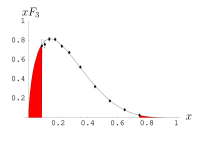
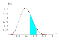
$$\qquad\!\!\!\!\times\frac{1}{x}\qquad\qquad\qquad\qquad\quad\qquad\;=\qquad$$

Figure 2: Constructing the Bernstein average, $F_{62}(Q^{2}=50.1\;{\rm{GeV}}^{2})$. The light grey region represents the interval in Eq. (66) and the dark grey areas represent the missing data regions. The small size of the dark grey region in the right hand plot demonstrates that this average will have negligible dependence on the missing data regions. Note that the right hand plot actually shows the integrand of the Bernstein average. The average itself will be this function integrated over $[0,1]$.

By expanding the integrand of Eq. (65) in powers of $x$, and using Eq. (1), we can relate the averages directly to the moments,

$$F_{nk}(Q^{2}) = \frac{2\Gamma(n+\frac{3}{2})}{\Gamma(k+\frac{1}{2})}\sum_{l=0}^{n-k}\frac{(-1)^{l}}{l!(n-k-l)!}{\cal M}(2(k+l)+1;Q^{2}),$$ (67)

and so theoretical predictions for the averages can be obtained by substitution of Eqs. (27), (24) and (36) into the above expression. The Bernstein average is seen to be a linear combination of odd moments. Due to the unavailability of results for $d_{2}$ for even $n$, previous NNLO analyses of this kind have been limited to the inclusion of only odd $F_{3}$ moments. However, now that the NNLO calculation of the NS anomalous dimension is complete [8, 9], we are no longer constrained in such a way. In light of this, we define a new set of modified Bernstein polynomials,

$$\qquad\tilde{p}_{nk}(x^{2}) = 2\frac{\Gamma\left(n+2\right)}{\Gamma\left(k+1\right)\Gamma\left(n-k+1\right)}x^{2k+1}(1-x^{2})^{n-k},\qquad n,k\in\mathbb{I},$$ (68)

which include only odd powers of $x$ and hence whose averages are related to even moments. These modified Bernstein polynomials are simply the original polynomials of Eq. (60), multiplied be $x$, and then ‘re-normalized’ such that they still satisfy $\int_{0}^{1}\tilde{p}_{nk}(x)dx=1$. We can calculate the mean and variance of $\tilde{p}_{nk}(x)$,

$$\overline{\tilde{x}} = \frac{\Gamma(k+\frac{3}{2})\Gamma(n+2)}{\Gamma(k+1)\Gamma(n+\frac{5}{2})},$$ (69)

$$\Delta\tilde{x} = \frac{k+1}{n+2}-\left[\frac{\Gamma(k+\frac{3}{2})\Gamma(n+2)}{\Gamma(k+1)\Gamma(n+\frac{5}{2})}\right]^{2},$$ (70)

and in analogy with Eq. (65), we define the modified Bernstein averages,

$$\tilde{F}_{nk}(Q^{2}) = \int_{0}^{1}\tilde{p}_{nk}(x^{2})F_{3}(x,Q^{2})dx.$$ (71)

Again, we only accept experimental modified averages for which the range,

$$\overline{\tilde{x}}_{nk}-\sqrt{\Delta\tilde{x}_{nk}}\;\leq\;x\;\leq\;\overline{\tilde{x}}_{nk}+\sqrt{\Delta\tilde{x}_{nk}},$$ (72)

lies within the region for which we have data. We obtain theoretical predictions for the modified averages using the equation,

$$\tilde{F}_{nk}(Q^{2}) = \frac{2\Gamma(n+2)}{\Gamma(k+1)}\sum_{l=0}^{n-k}\frac{(-1)^{l}}{l!(n-k-l)!}{\cal M}(2(k+l)+2;Q^{2}),$$ (73)

which is seen to be a linear combination of even moments.

In order to calculate averages from data for $F_{3}$, we need an expression for $xF_{3}$ covering the entire range of $x$, for each value of $Q^{2}$. As mentioned above, the values of the moments calculated in this way will depend on how we model the structure functions in the missing data regions but for the averages, this dependence is suppressed. However, we would like to test this assertion, and so we use four different methods of modelling $F_{3}$ and perform our analysis separately for each method. Significant differences between the results would signify a failure of the Bernstein average method, and in instances where this is the case, we reject that particular average at that particular $Q^{2}$. Moderate deviation however, is acceptable, provided that we use the magnitude of the deviation as an estimate of the error associated with the missing data region. This error is then included as a ‘modelling error’ in the final result. In this way, we can almost completely remove any dependence on missing data regions, and also quantify the error associated with any residual dependence.

The four extrapolation methods we use are described below:

1. In the first method, we fit the function,

   $$xF_{3}(x) = {\cal{A}}x^{\cal{B}}(1-x)^{\cal{C}},$$ (74)

   to the data for each fixed value of $Q^{2}$. The parameters ${\cal{A}}$, ${\cal{B}}$ and ${\cal{C}}$ are obtained by performing $\chi^{2}$ fitting of Eq. (74) to data for $F_{3}$. They are $Q^{2}$-dependent quantities, and errors on their values are obtained by performing the fitting with the data for $F_{3}$ shifted to the two extremes of the error bars.

   A justification for the particular form of fitting function in Eq. (74) can be found in Ref. [30]. However, the simple fact that this function fits the data well is justification enough, since the Bernstein averages are independent of the extrapolation method.

2. The second method we use is linear interpolation between successive data points. We also extrapolate beyond the data range, to the endpoints $xF_{3}(x)|_{x=0}=xF_{3}(x)|_{x=1}=0$, in order to be consistent with method I.

3. The third method consists of using the fitting function of Eq. (74), but setting $xF_{3}(x)=0$ everywhere outside the region for which we have data.

4. In analogy with III, in this method we use the linear interpolation of method II but setting $xF_{3}(x)=0$ everywhere outside the data region.

The deviation between the results obtained from the above methods (in particular, the difference between the first two and the last two) will be a good measure of the effectiveness of the Bernstein average method.

Data for $xF_{3}$ in neutrino-nucleon scattering is available from the CCFR collaboration [1]. The data was obtained from the scattering of neutrinos off iron nuclei and the measurements span the ranges $1.26\leq Q^{2}\leq 199.5\;{\rm{GeV}}^{2}$ and $0.015\leq x\leq 0.75$. The $x$-ranges covered at each $Q^{2}$ are depicted in Fig. 3.

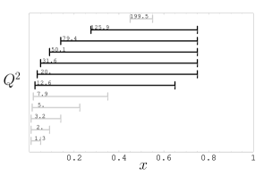
Figure 3: Diagram depicting the $x$-ranges covered by the CCFR data, at different $Q^{2}$.

In Fig. 4 we show each of the four modelling methods applied to $F_{3}$ measured at $Q^{2}=79.4\;{\rm{GeV}}^{2}$. Also shown on these figures (in grey) are the fits which are used to determine the errors on the modelling, which propagate through to errors on the averages.

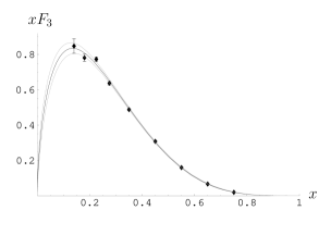
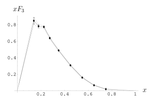
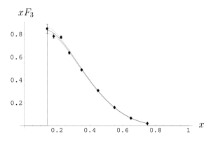
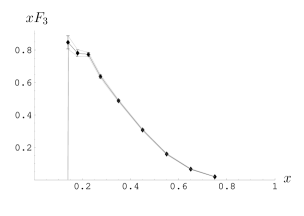
Figure 4: The four methods used for fitting the structure functions. Here we show the measured values of $xF_{3}$ at $Q^{2}=79.4\;{\rm GeV}^{2}$. The errors are determined by re-performing the fitting for the data shifted to the extremes of the error bars, and this is denoted by grey lines.

From the CCFR (and using the methods I - IV outlined above) we can obtain expressions describing the behaviour of the structure function over the full range of $x$, for each value of $Q^{2}$. It is then possible to extract experimental values of the averages, using the methods outlined below:

In the case of I, obtaining the averages is particularly simple. Substituting Eq. (74) into Eqs. (65) and (71) gives,

$$F^{(\textrm{\scriptsize{exp}})}_{nk} = \mathcal{A}\frac{2\Gamma(n+\frac{3}{2})}{\Gamma(k+\frac{1}{2})}\sum_{l=0}^{n-k}\frac{(-1)^{l}}{l!(n-k-l)!}{\rm B}(2(k+l)+\mathcal{B},\mathcal{C}+1),$$ (75)

for the Bernstein averages and,

$$\tilde{F}^{(\textrm{\scriptsize{exp}})}_{nk} = \mathcal{A}\frac{2\Gamma(n+2)}{\Gamma(k+1)}\sum_{l=0}^{n-k}\frac{(-1)^{l}}{l!(n-k-l)!}{\rm B}(2(k+l)+\mathcal{B}+1,\mathcal{C}+1),$$ (76)

for the modified Bernstein averages. Here, B$(x,y)\equiv\Gamma(x)\Gamma(y)/\Gamma(x+y)$ is the Beta function. Once values for ${\cal{A}}$, ${\cal{B}}$, and ${\cal{C}}$, have been obtained, substitution into the above expressions leads directly to the averages.

In the case of II, each of the averages is split into $j+1$ sections (where $j$ is the number of data points) and each section is an integral over a polynomial of order $2n+1$. It is then reasonably simple to evaluate the averages by computing this set of integrals. This approach also applies to method IV, but in this case there are only $j-1$ integrals.

For method III we simply integrate the fitting function, multiplied by the Bernstein polynomials, with the integration limits being the values of $x$ at the first and last data point.

Having outlined the method for obtaining the experimental averages we now turn our attention to which averages are acceptable at which energies. The highest moment we use is the 18th moment and the lowest the 1st. Inclusion of higher moments than this leads to no significant increase in the number of acceptable Bernstein averages. The upper limit of $n=18$ implies that the highest Bernstein averages included are $F_{8k}$ and $\tilde{F}_{8k}$ and that the lowest used are $F_{10}$ and $\tilde{F}_{10}$. We exclude the averages for which $n=k$ as they simply correspond to individual moments themselves. This leaves us with a total of 72 (36 + $\tilde{36}$) potential averages at our disposal for each value of $Q^{2}$. This number will be reduced when we come to exclude averages on the basis of the acceptance criteria. After applying the acceptance criteria, we are left with 132 data points for the standard Bernstein averages and 141 for the modified Bernstein averages. Exactly which averages we use at a particular $Q^{2}$, can be determined by inspecting the plots in the results section.

In Fig. 5 we plot the dominant regions of the Bernstein polynomials (given by Eq. (66)) for each of the used averages. This is superimposed onto the data-range diagram of Fig. 3. Figure 6 shows equivalent plots for the modified Bernstein averages. These plots can be used to identify which averages are acceptable for a particular value of $Q^{2}$.

\psfrag{x}{$x$}\psfrag{Qt}{{\scriptsize$\!\!\!\!Q^{2}/{\rm GeV}^{2}$}}\psfrag{F10}{{\color[rgb]{1,1,1}\scriptsize{$\!\!\!\!F_{10}$}}}\psfrag{F20}{{\color[rgb]{1,1,1}\scriptsize{$\!\!\!\!F_{20}$}}}\psfrag{F30}{{\color[rgb]{1,1,1}\scriptsize{$\!\!\!\!F_{30}$}}}\psfrag{F40}{{\color[rgb]{1,1,1}\scriptsize{$\!\!\!\!F_{40}$}}}\psfrag{F50}{{\color[rgb]{1,1,1}\scriptsize{$\!\!\!\!F_{50}$}}}\psfrag{F60}{{\color[rgb]{1,1,1}\scriptsize{$\!\!\!\!F_{60}$}}}\psfrag{F70}{{\color[rgb]{1,1,1}\scriptsize{$\!\!\!\!F_{70}$}}}\psfrag{F80}{{\color[rgb]{1,1,1}\scriptsize{$\!\!\!\!F_{80}$}}}\psfrag{F87}{{\color[rgb]{0,0,0}\scriptsize{$\!\!\!\!F_{87}$}}}\includegraphics[width=216.10109pt]{accept1.eps}

\psfrag{x}{$x$}\psfrag{Qt}{{\scriptsize$\!\!\!\!Q^{2}/{\rm GeV}^{2}$}}\psfrag{F21}{{\color[rgb]{1,1,1}\scriptsize{$\!\!\!\!F_{21}$}}}\psfrag{F31}{{\color[rgb]{1,1,1}\scriptsize{$\!\!\!\!F_{31}$}}}\psfrag{F41}{{\color[rgb]{1,1,1}\scriptsize{$\!\!\!\!F_{41}$}}}\psfrag{F51}{{\color[rgb]{1,1,1}\scriptsize{$\!\!\!\!F_{51}$}}}\psfrag{F61}{{\color[rgb]{1,1,1}\scriptsize{$\!\!\!\!F_{61}$}}}\psfrag{F71}{{\color[rgb]{1,1,1}\scriptsize{$\!\!\!\!F_{71}$}}}\psfrag{F81}{{\color[rgb]{1,1,1}\scriptsize{$\!\!\!\!F_{81}$}}}\psfrag{F76}{{\color[rgb]{0,0,0}\scriptsize{$\!\!\!\!F_{76}$}}}\psfrag{F86}{{\color[rgb]{0,0,0}\scriptsize{$\!\!\!\!F_{86}$}}}\includegraphics[width=216.10109pt]{accept2.eps}

\psfrag{x}{$x$}\psfrag{Qt}{{\scriptsize$\!\!\!\!Q^{2}/{\rm GeV}^{2}$}}\psfrag{F32}{{\color[rgb]{1,1,1}\scriptsize{$\!\!\!\!F_{32}$}}}\psfrag{F42}{{\color[rgb]{1,1,1}\scriptsize{$\!\!\!\!F_{42}$}}}\psfrag{F52}{{\color[rgb]{1,1,1}\scriptsize{$\!\!\!\!F_{52}$}}}\psfrag{F62}{{\color[rgb]{1,1,1}\scriptsize{$\!\!\!\!F_{62}$}}}\psfrag{F72}{{\color[rgb]{1,1,1}\scriptsize{$\!\!\!\!F_{72}$}}}\psfrag{F82}{{\color[rgb]{1,1,1}\scriptsize{$\!\!\!\!F_{82}$}}}\psfrag{F65}{{\color[rgb]{0,0,0}\scriptsize{$\!\!\!\!F_{65}$}}}\psfrag{F75}{{\color[rgb]{0,0,0}\scriptsize{$\!\!\!\!F_{75}$}}}\psfrag{F85}{{\color[rgb]{0,0,0}\scriptsize{$\!\!\!\!F_{85}$}}}\includegraphics[width=216.10109pt]{accept3.eps}

\psfrag{x}{$x$}\psfrag{Qt}{{\scriptsize$\!\!\!\!Q^{2}/{\rm GeV}^{2}$}}\psfrag{F43}{{\color[rgb]{1,1,1}\scriptsize{$\!\!\!\!F_{43}$}}}\psfrag{F53}{{\color[rgb]{1,1,1}\scriptsize{$\!\!\!\!F_{53}$}}}\psfrag{F63}{{\color[rgb]{1,1,1}\scriptsize{$\!\!\!\!F_{63}$}}}\psfrag{F73}{{\color[rgb]{1,1,1}\scriptsize{$\!\!\!\!F_{73}$}}}\psfrag{F83}{{\color[rgb]{1,1,1}\scriptsize{$\!\!\!\!F_{83}$}}}\psfrag{F54}{{\color[rgb]{0,0,0}\scriptsize{$\!\!\!\!F_{54}$}}}\psfrag{F64}{{\color[rgb]{0,0,0}\scriptsize{$\!\!\!\!F_{64}$}}}\psfrag{F74}{{\color[rgb]{0,0,0}\scriptsize{$\!\!\!\!F_{74}$}}}\psfrag{F84}{{\color[rgb]{0,0,0}\scriptsize{$\!\!\!\!F_{84}$}}}\includegraphics[width=216.10109pt]{accept4.eps}

Figure 5: The black and light grey bars ($\vdash\!\dashv$) show $x$ ranges covered by the CCFR data at different energies. Superimposed onto these, in various colours, are the peaked regions of the individual Bernstein polynomials, defined by the interval in Eq. (66).

\psfrag{x}{$x$}\psfrag{Qt}{{\scriptsize$\!\!\!\!Q^{2}/{\rm GeV}^{2}$}}\psfrag{F10}{{\color[rgb]{1,1,1}\tiny{$\!\!\!\!\tilde{F}_{10}$}}}\psfrag{F20}{{\color[rgb]{1,1,1}\tiny{$\!\!\!\!\tilde{F}_{20}$}}}\psfrag{F30}{{\color[rgb]{1,1,1}\tiny{$\!\!\!\!\tilde{F}_{30}$}}}\psfrag{F40}{{\color[rgb]{1,1,1}\tiny{$\!\!\!\!\tilde{F}_{40}$}}}\psfrag{F50}{{\color[rgb]{1,1,1}\tiny{$\!\!\!\!\tilde{F}_{50}$}}}\psfrag{F60}{{\color[rgb]{1,1,1}\tiny{$\!\!\!\!\tilde{F}_{60}$}}}\psfrag{F70}{{\color[rgb]{1,1,1}\tiny{$\!\!\!\!\tilde{F}_{70}$}}}\psfrag{F80}{{\color[rgb]{1,1,1}\tiny{$\!\!\!\!\tilde{F}_{80}$}}}\psfrag{F87}{{\color[rgb]{0,0,0}\tiny{$\!\!\!\!\tilde{F}_{87}$}}}\includegraphics[width=216.10109pt]{accept1x.eps}

\psfrag{x}{$x$}\psfrag{Qt}{{\scriptsize$\!\!\!\!Q^{2}/{\rm GeV}^{2}$}}\psfrag{F21}{{\color[rgb]{1,1,1}\tiny{$\!\!\!\!\tilde{F}_{21}$}}}\psfrag{F31}{{\color[rgb]{1,1,1}\tiny{$\!\!\!\!\tilde{F}_{31}$}}}\psfrag{F41}{{\color[rgb]{1,1,1}\tiny{$\!\!\!\!\tilde{F}_{41}$}}}\psfrag{F51}{{\color[rgb]{1,1,1}\tiny{$\!\!\!\!\tilde{F}_{51}$}}}\psfrag{F61}{{\color[rgb]{1,1,1}\tiny{$\!\!\!\!\tilde{F}_{61}$}}}\psfrag{F71}{{\color[rgb]{1,1,1}\tiny{$\!\!\!\!\tilde{F}_{71}$}}}\psfrag{F81}{{\color[rgb]{1,1,1}\tiny{$\!\!\!\!\tilde{F}_{81}$}}}\psfrag{F76}{{\color[rgb]{0,0,0}\tiny{$\!\!\!\!\tilde{F}_{76}$}}}\psfrag{F86}{{\color[rgb]{0,0,0}\tiny{$\!\!\!\!\tilde{F}_{86}$}}}\includegraphics[width=216.10109pt]{accept2x.eps}

\psfrag{x}{$x$}\psfrag{Qt}{{\scriptsize$\!\!\!\!Q^{2}/{\rm GeV}^{2}$}}\psfrag{F32}{{\color[rgb]{1,1,1}\tiny{$\!\!\!\!\tilde{F}_{32}$}}}\psfrag{F42}{{\color[rgb]{1,1,1}\tiny{$\!\!\!\!\tilde{F}_{42}$}}}\psfrag{F52}{{\color[rgb]{1,1,1}\tiny{$\!\!\!\!\tilde{F}_{52}$}}}\psfrag{F62}{{\color[rgb]{1,1,1}\tiny{$\!\!\!\!\tilde{F}_{62}$}}}\psfrag{F72}{{\color[rgb]{1,1,1}\tiny{$\!\!\!\!\tilde{F}_{72}$}}}\psfrag{F82}{{\color[rgb]{1,1,1}\tiny{$\!\!\!\!\tilde{F}_{82}$}}}\psfrag{F65}{{\color[rgb]{0,0,0}\tiny{$\!\!\!\!\tilde{F}_{65}$}}}\psfrag{F75}{{\color[rgb]{0,0,0}\tiny{$\!\!\!\!\tilde{F}_{75}$}}}\psfrag{F85}{{\color[rgb]{0,0,0}\tiny{$\!\!\!\!\tilde{F}_{85}$}}}\includegraphics[width=216.10109pt]{accept3x.eps}

\psfrag{x}{$x$}\psfrag{Qt}{{\scriptsize$\!\!\!\!Q^{2}/{\rm GeV}^{2}$}}\psfrag{F43}{{\color[rgb]{1,1,1}\tiny{$\!\!\!\!\tilde{F}_{43}$}}}\psfrag{F53}{{\color[rgb]{1,1,1}\tiny{$\!\!\!\!\tilde{F}_{53}$}}}\psfrag{F63}{{\color[rgb]{1,1,1}\tiny{$\!\!\!\!\tilde{F}_{63}$}}}\psfrag{F73}{{\color[rgb]{1,1,1}\tiny{$\!\!\!\!\tilde{F}_{73}$}}}\psfrag{F83}{{\color[rgb]{1,1,1}\tiny{$\!\!\!\!\tilde{F}_{83}$}}}\psfrag{F54}{{\color[rgb]{0,0,0}\tiny{$\!\!\!\!\tilde{F}_{54}$}}}\psfrag{F64}{{\color[rgb]{0,0,0}\tiny{$\!\!\!\!\tilde{F}_{64}$}}}\psfrag{F74}{{\color[rgb]{0,0,0}\tiny{$\!\!\!\!\tilde{F}_{74}$}}}\psfrag{F84}{{\color[rgb]{0,0,0}\tiny{$\!\!\!\!\tilde{F}_{84}$}}}\includegraphics[width=216.10109pt]{accept4x.eps}

Figure 6: The black and light grey bars ($\vdash\!\dashv$) show $x$ ranges covered by the CCFR data at different energies. Superimposed onto these, in various colours, are the peaked regions of the individual modified Bernstein polynomials, defined by the interval in Eq. (72).

5 Fitting procedure

We use $\chi^{2}$ minimization to optimize the fits of the theoretical predictions to the data. The highest moment included in the experimental averages is the 18th, and so when TMCs are included, we will require predictions for the first 20 moments. Therefore, the set of fitting parameters comprises of $\{A_{1}\ldots A_{20}\}$ plus the QCD scale parameter $\Lambda_{\textrm{\tiny{$\overline{{\rm MS}}$}}}$. When we include higher twist corrections this set is expanded to include $A_{\textrm{\tiny{HT}}}$. To check consistency between the odd and even moments we perform the analysis for each of these sets of moments separately and then finally together, and compare the results.

Although we stated previously that 132 standard Bernstein averages are available to us, in the CORGI case this is reduced to 130 for the following reason: When fitting predictions to the data, we scan values of $\Lambda_{\textrm{\tiny{$\overline{{\rm MS}}$}}}^{(4)}$ between 0 and 590 MeV for a minimum in $\chi^{2}$. Unfortunately, for $n=17$ and 19, the values of $\Lambda_{{\cal M}}/\Lambda_{\textrm{\tiny{$\overline{{\rm MS}}$}}}$ (see table 1) are such that $Q^{2}=7.9\;{\rm GeV}^{2}$ is below the Landau pole in Eq. (28). Consequently we cannot obtain CORGI predictions for Bernstein averages which include these moments. From Eqs. (52) and (67) we can determine that this excludes $F_{80}(Q^{2}=7.9\;{\rm{GeV}}^{2})$ and $F_{70}(Q^{2}=7.9\;{\rm{GeV}}^{2})$ from the fit. In the case of the modified Bernstein averages, $\tilde{F}_{80}(Q^{2}=7.9\;{\rm{GeV}}^{2})$ and $\tilde{F}_{70}(Q^{2}=7.9\;{\rm{GeV}}^{2})$ are already excluded due to their failure to meet the acceptance criteria.

The CCFR data includes statistical errors and 18 different sources of systematic error. These errors cannot be added in quadrature, and so we perform the analysis for each of these 19 sources of error separately and then add the variation in the results in quadrature to obtain the final total error. We also include, as additional sources of error the deviation in results associated with using the four different modelling methods (this forms the ‘modelling error’ in our final result), and the deviation in the results obtained from performing the analysis with and without HT corrections included (forming the ‘HT error’).

Correlation of errors

When fitting theoretical predictions to experimental data using $\chi^{2}$ minimization, care must be taken in order to take into account fully the correlation between data points.

To construct $\chi^{2}$ from a set of $N$ uncorrelated data points $\{f_{i}^{\textrm{\tiny{exp.}}}\}$ ($i=1,\ldots N$), with errors $\{\sigma_{f_{i}}\}$ and corresponding theoretical predictions $\{f_{i}^{\textrm{\tiny{theo.}}}\}$, we have,

$$\chi^{2} = \sum_{i=1}^{N}\left(\frac{f_{i}^{\textrm{\tiny{exp.}}}-f_{i}^{\textrm{\tiny{theo.}}}}{\sigma_{f_{i}}}\right)^{2}.$$ (77)

The raw data for $xF_{3}$ are uncorrelated. However, we are not comparing predictions for the structure functions themselves with data directly; rather we are doing so indirectly via the Bernstein averages. For a given value of $Q^{2}$, the full set of Bernstein averages (and modified Bernstein averages) we obtain will be correlated, due to their being derived from the same set of ($xF_{3}$) data points (see Fig. 2).

In the case where $\{f_{i}^{\textrm{\tiny{exp.}}}\}$ are correlated the $\chi^{2}$ function becomes [26],

$$\chi^{2} = \sum_{i=1}^{N}\sum_{j=1}^{N}\left(f_{i}^{\textrm{\tiny{exp.}}}-f_{i}^{\textrm{\tiny{theo.}}}\right)V^{-1}_{ij}\left(f_{j}^{\textrm{\tiny{exp.}}}-f_{j}^{\textrm{\tiny{theo.}}}\right)$$ (78)

$$= \left(\textbf{f}^{\;\textrm{\tiny{exp.}}}-\textbf{f}^{\;\textrm{\tiny{theo.}}}\right)^{T}\textbf{V}^{-1}\left(\textbf{f}^{\;\textrm{\tiny{exp.}}}-\textbf{f}^{\;\textrm{\tiny{theo.}}}\right).$$

In the second line of the above equation we have constructed vectors from the data points and their predictions. V is known as the covariance matrix. It encodes the correlation between each of the data points; its elements are obtained as follows,

$$V_{ij} = {\rm cov}\left(f_{i},f_{j}\right)$$ (79)

$$= \langle f_{i}f_{j}\rangle-\langle f_{i}\rangle\langle f_{j}\rangle.$$

If the $f_{i}$ are themselves functions of $M$ variables $x_{k}$ (representing the ‘raw’ data), then we have,

$${\rm cov}\left(f_{k},f_{l}\right) = \sum_{i=1}^{M}\sum_{j=1}^{M}\left(\frac{\partial f_{k}}{\partial x_{i}}\right)\left(\frac{\partial f_{l}}{\partial x_{j}}\right){\rm cov}\left(x_{i},x_{j}\right).$$ (80)

If the data for $x_{i}$ are uncorrelated, this reduces to,

$${\rm cov}\left(f_{k},f_{l}\right) = \sum_{i=1}^{M}\left(\frac{\partial f_{k}}{\partial x_{i}}\right)\left(\frac{\partial f_{l}}{\partial x_{i}}\right)\sigma_{x_{i}}^{2}.$$ (81)

To obtain the covariance of the Bernstein averages we simply substitute $F_{nk}(Q^{2})$ for $f_{i}$ and $F_{3}(x)$ for $x_{i}$ in Eq. (81). We assume no correlation between different values of $Q^{2}$ and so Eq. (78) decouples into 7 different matrix equations (one for each of the values of $Q^{2}$ between 7.9 and 125.9 ${\rm GeV}^{2}$). By using the trapezium rule to approximate the Bernstein average integrals, we obtain the following expression for the covariance matrices:

$$V_{lm}(Q_{i}^{2}) = \sum_{j=1}^{N_{i}}\frac{1}{4}\left(p_{nk}(x_{j})\right)_{l}\left(p_{nk}(x_{j})\right)_{m}\left(x_{j+1}-x_{j-1}\right)^{2}\sigma_{F_{3}(x_{j})}^{2}.$$ (82)

Here, the index $j$ runs over the number of data points we have for $xF_{3}$ at a given $Q_{i}^{2}$. The $j=0$ and $j=N_{i}+1$ terms are simply the $x=0$ and $x=1$ endpoints (see parts I and II of Fig. 4). From this equation we can calculate elements of the covariance matrices for each value of $Q^{2}$. All that remains is for us to invert them. However, upon attempting to do so, we find that these matrices are ill-conditioned, with some of their eigenvalues being close to zero. Hence their inverses are intractable. As a result of this, it is impossible to perform a reliable $\chi^{2}$ analysis of the averages with their correlation taken into account.

We believe that this is principally due to the fact that the correlation between averages is significant in some cases, and this in turn is an artefact of the fact that the selection criteria systematically select Bernstein polynomials which are peaked in the same region and hence are of fairly similar shape. This situation arises because the intent behind the inclusion of more averages in the analysis is not to increase the amount of ‘data’, rather it is to further ensure that the missing data regions are suppressed.

In light of this, we settle for the method adopted in Refs. [3, 4], in which the naïve $\chi^{2}$ function of Eq. (77) is used, but the error bars on the averages are modified in order to account for the ‘over-counting of degrees of freedom’. For example, for the standard averages, at each value of $Q^{2}$ we have theoretical information on 9 moments, but the number of experimental Bernstein averages we use is often more than this; e.g. for $Q^{2}=20\,{\rm GeV}^{2}$ we use 27 standard Bernstein averages. To remedy this, we adopt the following approach. For each value of $Q^{2}$ we count the number of averages above 9 as duplicate information. The number of duplicates we have altogether is 73 and so for the values of $Q^{2}$ for which we have more Bernstein averages than moments, we rescale the error on these averages by $\sqrt{130/(130-73)}=1.510$. Correspondingly, for the modified Bernstein averages we rescale the errors by a factor of $\sqrt{141/(141-87)}=1.616$. This rescaling has the effect of suppressing the contribution of the duplicate data points to $\chi^{2}$, relative to those values of $Q^{2}$ for which we have fewer Bernstein averages than moments.

Positivity constraints

The fact that $xF_{3}$ is a positive definite function, and that the moments are simply integrals over these functions multiplied by a single power of $x$, means that we can impose certain positivity constraints on the parameters $A_{n}$, as follows.

We construct the following matrices from the moments,

$$\hat{{\cal M}}\;=\;\left(\begin{array}[]{cccc}{\cal M}_{1}&{\cal M}_{2}&\cdots&{\cal M}_{9}\\[5.0pt] {\cal M}_{2}&{\cal M}_{3}&&\\ {\cal M}_{3}&&\ddots&\\ \vdots&&&\\ {\cal M}_{9}&&&{\cal M}_{17}\\ \end{array}\right),$$ (88)

and

$$\Delta\hat{{\cal M}}\;=\;\left(\begin{array}[]{cccc}\Delta{\cal M}_{1}&\Delta{\cal M}_{2}&\cdots&\Delta{\cal M}_{9}\\[5.0pt] \Delta{\cal M}_{2}&\Delta{\cal M}_{3}&&\\ \Delta{\cal M}_{3}&&\ddots&\\ \vdots&&&\\ \Delta{\cal M}_{9}&&&\Delta{\cal M}_{17}\\ \end{array}\right),$$ (94)

where ${\cal M}_{n}={\cal M}(n;Q^{2})$ and $\Delta{\cal M}_{n}={\cal M}_{n}-{\cal M}_{n+1}$.

In order for ${\cal M}(n;Q^{2})$ to be moments of positive definite functions (as the structure functions must be), the determinants of the above matrices, and of all their minors, must be positive, for all values of $Q^{2}$ [4]. Evaluating these determinants at fixed $Q^{2}$ will translate to conditions on the parameters $A_{n}$. We do not implement these constraints as part of the fitting procedure. Rather, we perform checks on the values of the fitting parameters resulting from the $\chi^{2}$ minimization to ensure that they obey the above constraints.

However, we do impose positivity constraints on the moments themselves. As a result of the determinantal constraints described above, and from the general form of the moments given in Eq. (1), we can infer that the following inequalities must be satisfied,

$${\cal M}(n;Q^{2}) > 0,$$ (95)

$${\cal M}(n;Q^{2}) > {\cal M}(n+1;Q^{2}),$$ (96)

for fixed $Q^{2}$. Furthermore, we can implement these constraints by defining our fitting parameters $A_{n}$ in terms of a new set of parameters and then minimizing $\chi^{2}$ with respect to these new parameters.

We begin by picking some value of $Q_{0}^{2}$ at which to implement the conditions. We then take the last moment used in the analysis ($n=20$) and rewrite the constraint in Eq. (95) as,

$${\cal M}(20;Q_{0}^{2}) = \left(\hat{A}_{20}\right)^{2},$$ (97)

where $\hat{A}_{20}$ is a real number. The constraints in Eq. (96) can also be rewritten as,

$${\cal M}(n;Q_{0}^{2}) = {\cal M}(n+1;Q_{0}^{2})+\left(\hat{A}_{n}\right)^{2},$$ (98)

for $1\leq n<20$, where $\hat{A}_{n}$ are all real numbers. The LHSs of Eqs. (97) and (98) are simply a fitting parameter times a number. For example, in the case of $n=2$ and $Q^{2}_{0}=12.6\;{\rm GeV}^{2}$ we have,

$${\cal M}(2;12.6\;{\rm GeV}^{2}) = 0.3932\,A_{2}.$$ (99)

From this, and equivalent expressions for the rest of $A_{n}$, we can obtain an expression for each $A_{n}$ in terms of the parameters $\hat{A}_{1}$ - $\hat{A}_{20}$. This means that we can replace the parameters $A_{1}$ - $A_{20}$ with $\hat{A}_{1}$ - $\hat{A}_{20}$ in the $\chi^{2}$ function. By doing this and then minimizing with respect to the $\hat{A}_{n}$ parameters, we can find a minimum in $\chi^{2}$ for which the constraints in Eqs. (95) and (96) are automatically satisfied. In effect, the reparameterization embedded in Eqs. (97) and (98) restricts the parameter space to exclude solutions for which the constraints are not satisfied.

To implement this reparameterization we must choose a value of $Q_{0}^{2}$ at which to impose the constraints, whereas in reality they must be satisfied for all $Q^{2}$. Because of this, we perform the analysis for several different values of $Q_{0}^{2}$ and check that the results remain stable.

6 Results of fitting to the data

We focus principally on the results from the CORGI analysis in which both odd and even moments are included and in which we include target mass corrections. This analysis results in a prediction for the QCD scale parameter of,

$$\Lambda_{\textrm{\tiny{$\overline{{\rm MS}}$}}}^{(5)} = 219.11_{-23.6}^{+22.1}\;{\rm MeV}.$$ (100)

The errors on this value can be broken down into four different sources,

$$\Lambda_{\textrm{\tiny{$\overline{{\rm MS}}$}}}^{(5)} = 219.11\;_{-16.57}^{+18.36}\;({\rm stat.})\quad_{-8.17}^{+8.36}\;({\rm sys.})\quad_{-13.74}^{+14.47}\;({\rm mod.})\quad\pm 8.97\;({\rm HT})\;{\rm MeV}.$$ (101)

We have used method I to obtain experimental values of the averages. The deviation between the results obtained using methods I and IV is used to evaluate the modelling error since these are the two methods which exhibit the largest deviation.

This result for $\Lambda_{\textrm{\tiny{$\overline{{\rm MS}}$}}}$ corresponds to a value of the strong coupling constant (evaluated at the mass of the $Z$ particle) of,

$$\alpha_{s}(M_{Z}) = 0.1189_{-0.0019}^{+0.0019}$$ (102)

These values are in excellent agreement with the current global averages of $\Lambda_{\textrm{\tiny{$\overline{{\rm MS}}$}}}^{(5)}=207.2\;{\rm GeV}$ and $\alpha_{s}=0.118\pm.002$ [24]. There is also good agreement with the result obtained from fits using the Jacobi polynomial method [13] which yield ${\alpha}_{s}(M_{Z})={0.119}^{+0.004}_{-0.004}$. This result is based on fits using odd moments only and includes a contribution to the error from scale dependence. Whilst close to the global average, the value of $\alpha_{s}(M_{Z})$ we obtain is significantly larger than the values found in a recent analysis of the $F_{2}(x,Q^{2})$ structure function [27], or from fits of parton distibution functions where DIS and Drell-Yan data are combined [28], it is also larger than the value which minimizes the $\chi^{2}$ in global parton distribution function fits such as Ref. [29].

The $\chi^{2}/$d.o.f. for our CORGI result is as follows,

$$\frac{\chi^{2}}{\rm d.o.f.} = \frac{20.37}{271-(20+1)}$$ (103)

$$= 0.0815.$$

Here ‘$271$’ refers to the number of experimental Bernstein average points used in the fits. Although this value is an order of magnitude larger than the $\chi^{2}/$d.o.f. obtained in Ref. [4], it is still significantly smaller than one would expect, suggesting the errors on the Bernstein averages have been over estimated. However, as discussed previously, the $\chi^{2}$ function we are using does not take into account the correlation between data points. Indeed, if correlation was taken into account, one might expect that a more reasonable value of $\chi^{2}$ would be obtained.

Furthermore, in the $\chi^{2}$ function we eventually used, the errors on the Bernstein averages were rescaled in order to take into account the ‘over-counting of degrees of freedom’. As a result, the number of Bernstein averages is not representative of the true number of degrees of freedom in this particular $\chi^{2}$ function. Indeed, the Bernstein averages in the plots in Fig. 7 can be constructed from just 58 different moments at different values of $Q^{2}$ (via Eq. (67)). Similarly, the modified Bernstein averages in Fig. 8 can be built from 53 different moments. Hence,

$$\frac{\chi^{2}}{\rm d.o.f.}\;=\;\frac{20.37}{111-21}\;=\;0.226,$$ (104)

is more representative of the true value of $\chi^{2}/$d.o.f. in this approach. This is a more acceptable value, however we stress that the true minimum in $\chi^{2}$ can only be determined by taking correlation fully into account.

In Fig. 7 we plot the CORGI predictions for the Bernstein averages (with TMCs included) fitted to the experimental values. Figure 8 shows equivalent plots for the modified averages.

\psfrag{Fb}{$F_{nk}$}\psfrag{F70}{{\color[rgb]{1,0,1}\small{$F_{70}$}}}\psfrag{F50}{{\color[rgb]{0,0,1}\small{$F_{50}$}}}\psfrag{F30}{{\color[rgb]{0.08860759493670886,0.8,0.16877637130801687}\small{$F_{30}$}}}\psfrag{F10}{{\color[rgb]{1,0,0}\small{$F_{10}$}}}\includegraphics[width=220.50885pt]{b1.eps}	\psfrag{Fb}{$F_{nk}$}\psfrag{F80}{{\color[rgb]{0.8,0,0}\small{$F_{80}$}}}\psfrag{F60}{{\color[rgb]{0.6,0.6,0}\small{$F_{60}$}}}\psfrag{F40}{{\color[rgb]{0,0.75,1}\small{$F_{40}$}}}\psfrag{F20}{{\color[rgb]{1,0,1}\small{$F_{20}$}}}\includegraphics[width=220.50885pt]{b2.eps}
$Q^{2}/{\rm GeV}^{2}$	$Q^{2}/{\rm GeV}^{2}$
\psfrag{Fb}{$F_{nk}$}\psfrag{F81}{{\color[rgb]{0.8,0,0}\small{$F_{81}$}}}\psfrag{F71}{{\color[rgb]{0.6,0.6,0}\small{$F_{71}$}}}\psfrag{F61}{{\color[rgb]{0,0.75,1}\small{$F_{61}$}}}\psfrag{F51}{{\color[rgb]{1,0,1}\small{$F_{51}$}}}\psfrag{F41}{{\color[rgb]{0,0,1}\small{$F_{41}$}}}\psfrag{F31}{{\color[rgb]{0.08860759493670886,0.8,0.16877637130801687}\small{$F_{31}$}}}\psfrag{F21}{{\color[rgb]{1,0,0}\small{$F_{21}$}}}\includegraphics[width=220.50885pt]{b3.eps}	\psfrag{Fb}{$F_{nk}$}\psfrag{F82}{{\color[rgb]{0.8,0,0}\small{$F_{82}$}}}\psfrag{F72}{{\color[rgb]{0.6,0.6,0}\small{$F_{72}$}}}\psfrag{F62}{{\color[rgb]{0,0.75,1}\small{$F_{62}$}}}\psfrag{F52}{{\color[rgb]{1,0,1}\small{$F_{52}$}}}\psfrag{F42}{{\color[rgb]{0,0,1}\small{$F_{42}$}}}\psfrag{F32}{{\color[rgb]{0.08860759493670886,0.8,0.16877637130801687}\small{$F_{32}$}}}\psfrag{F74}{{\color[rgb]{1,0,0}\small{$F_{74}$}}}\includegraphics[width=220.50885pt]{b4.eps}
$Q^{2}/{\rm GeV}^{2}$	$Q^{2}/{\rm GeV}^{2}$
\psfrag{Fb}{$F_{nk}$}\psfrag{F83}{{\color[rgb]{0,0.75,1}\small{$F_{83}$}}}\psfrag{F73}{{\color[rgb]{1,0,1}\small{$F_{73}$}}}\psfrag{F63}{{\color[rgb]{0,0,1}\small{$F_{63}$}}}\psfrag{F84}{{\color[rgb]{0.08860759493670886,0.8,0.16877637130801687}\small{$F_{84}$}}}\psfrag{F53}{{\color[rgb]{1,0,0}\small{$F_{53}$}}}\includegraphics[width=220.50885pt]{b5.eps}
$Q^{2}/{\rm GeV}^{2}$

Figure 7: CORGI fits for the Bernstein averages, with TMCs included.

\psfrag{Fb}{$\tilde{F}_{nk}$}\psfrag{F90}{{\color[rgb]{0.08860759493670886,0.8,0.16877637130801687}\small{$\tilde{F}_{80}$}}}\psfrag{F80}{{\color[rgb]{0.8,0,0}\small{$\tilde{F}_{80}$}}}\psfrag{F70}{{\color[rgb]{0.8,0,0}\small{$\tilde{F}_{70}$}}}\psfrag{F60}{{\color[rgb]{0.6,0.6,0}\small{$\tilde{F}_{60}$}}}\psfrag{F50}{{\color[rgb]{0,0.75,1}\small{$\tilde{F}_{50}$}}}\psfrag{F40}{{\color[rgb]{1,0,1}\small{$\tilde{F}_{40}$}}}\psfrag{F30}{{\color[rgb]{0,0,1}\small{$\tilde{F}_{30}$}}}\psfrag{F20}{{\color[rgb]{0.08860759493670886,0.8,0.16877637130801687}\small{$\tilde{F}_{20}$}}}\psfrag{F10}{{\color[rgb]{1,0,0}\small{$\tilde{F}_{10}$}}}\includegraphics[width=220.50885pt]{mb1.eps}	\psfrag{Fb}{$\tilde{F}_{nk}$}\psfrag{F81}{{\color[rgb]{0.8,0,0}\small{$\tilde{F}_{81}$}}}\psfrag{F71}{{\color[rgb]{0.6,0.6,0}\small{$\tilde{F}_{71}$}}}\psfrag{F61}{{\color[rgb]{0,0.75,1}\small{$\tilde{F}_{61}$}}}\psfrag{F51}{{\color[rgb]{1,0,1}\small{$\tilde{F}_{51}$}}}\psfrag{F41}{{\color[rgb]{0,0,1}\small{$\tilde{F}_{41}$}}}\psfrag{F31}{{\color[rgb]{0.08860759493670886,0.8,0.16877637130801687}\small{$\tilde{F}_{31}$}}}\psfrag{F21}{{\color[rgb]{1,0,0}\small{$\tilde{F}_{21}$}}}\includegraphics[width=220.50885pt]{mb2.eps}
$Q^{2}/{\rm GeV}^{2}$	$Q^{2}/{\rm GeV}^{2}$
\psfrag{Fb}{$\tilde{F}_{nk}$}\psfrag{F82}{{\color[rgb]{0.8,0,0}\small{$\tilde{F}_{82}$}}}\psfrag{F72}{{\color[rgb]{0.6,0.6,0}\small{$\tilde{F}_{72}$}}}\psfrag{F62}{{\color[rgb]{0,0.75,1}\small{$\tilde{F}_{62}$}}}\psfrag{F52}{{\color[rgb]{1,0,1}\small{$\tilde{F}_{52}$}}}\psfrag{F42}{{\color[rgb]{0,0,1}\small{$\tilde{F}_{42}$}}}\psfrag{F84}{{\color[rgb]{0.08860759493670886,0.8,0.16877637130801687}\small{$\tilde{F}_{84}$}}}\psfrag{F74}{{\color[rgb]{1,0,0}\small{$\tilde{F}_{74}$}}}\includegraphics[width=220.50885pt]{mb3.eps}	\psfrag{Fb}{$\tilde{F}_{nk}$}\psfrag{F83}{{\color[rgb]{1,0,1}\small{$\tilde{F}_{83}$}}}\psfrag{F73}{{\color[rgb]{0,0,1}\small{$\tilde{F}_{73}$}}}\psfrag{F63}{{\color[rgb]{0.08860759493670886,0.8,0.16877637130801687}\small{$\tilde{F}_{63}$}}}\psfrag{F53}{{\color[rgb]{1,0,0}\small{$\tilde{F}_{53}$}}}\includegraphics[width=220.50885pt]{mb4.eps}
$Q^{2}/{\rm GeV}^{2}$	$Q^{2}/{\rm GeV}^{2}$

Figure 8: CORGI fits for the modified Bernstein averages, with TMCs included.

	$\Lambda_{\textrm{\tiny{$\overline{{\rm MS}}$}}}^{(5)}(\textrm{MeV})$	$\alpha_{s}(M_{Z})$	$\chi^{2}/{\rm d.o.f.}$
All moments	219.1$\begin{array}[]{l}\!\!\!+23.6\\ \!\!\!-22.1\end{array}$	0.1189$\begin{array}[]{l}\!\!\!+0.0019\\ \!\!\!-0.0019\end{array}$	$20.37/(271-(20+1))$
Odd moments	210.5$\begin{array}[]{l}\!\!\!+35.0\\ \!\!\!-32.7\end{array}$	0.1182$\begin{array}[]{l}\!\!\!+0.0029\\ \!\!\!-0.0030\end{array}$	$10.94/(130-(10+1))$
Even moments	229.5$\begin{array}[]{l}\!\!\!+64.7\\ \!\!\!-62.1\end{array}$	0.1198$\begin{array}[]{l}\!\!\!+0.0048\\ \!\!\!-0.0048\end{array}$	$9.24/(141-(10+1))$
All moments: $Q^{2}>m_{b}^{2}$ only	232.4$\begin{array}[]{l}\!\!\!+34.9\\ \!\!\!-33.2\end{array}$	0.1200$\begin{array}[]{l}\!\!\!+0.0027\\ \!\!\!-0.0027\end{array}$	$15.59/(228-(20+1))$

Table 2: In this table we present the result of the analysis performed using the CORGI approach to perturbation theory with target mass corrections included. We compare the results obtained when we include all moments (up to $n=20$) with those obtained when we restrict the analysis to even or odd moments only. We also show the results from performing the analysis with only data points for which $Q^{2}>m_{b}^{2}$ ($N_{f}=5$) included.

In table 2 we present the full set of results from the CORGI analysis. This table shows the results obtained when we include both odd and even moments (standard and modified Bernstein averages) together and also when we restrict the analysis to odd and even or odd moments only. These results allow us to check consistency between the odd, even and ‘All’ analyses.

We can also use the results of the ‘odd moments’ analysis to check consistency with previous analyses. In the PS analysis of Ref. [4] (in which only the $n=1,3,5,7,9,11$ and 13 moments were included) a value of $\Lambda_{\textrm{\tiny{$\overline{{\rm MS}}$}}}^{(4)}=255\pm 72$MeV was found, corresponding to $\Lambda_{\textrm{\tiny{$\overline{{\rm MS}}$}}}^{(5)}=178_{-55}^{+57}$MeV, with a value of $\chi^{2}/{\rm d.o.f.}=0.007$. Using the same set of moments, the CORGI analysis of Ref. [5] found a value of $\Lambda_{\textrm{\tiny{$\overline{{\rm MS}}$}}}^{(5)}=228_{-36}^{+35}$MeV, although it must be noted that this analysis used incorrect values of the coefficients $X_{2}$, and therefore the result must be regarded as unreliable. Both of those results are indeed consistent with the ‘odd moments’ analysis performed here.

We also perform an analysis in which we restrict the CCFR data to $Q^{2}>m_{b}^{2}$ only, as a check on our method of evolving through the $b$ quark threshold. These results are also included in table 2. In table 3 we give the fitted CORGI values for the $A_{n}$ non-perturbative coefficients for $n=1-20$, together with the values of the corresponding moments at $Q^{2}={8.75}\;{\rm{GeV}}^{2}$ and ${12.6}\;{\rm{GeV}}^{2}$.

In table 4 we compare the CORGI results with those obtained using the PS and EC approaches. We also present results obtained from performing these analyses with and without target mass corrections. The fact that the number of d.o.f. for the CORGI fits is $271$ ($272$), as opposed to $273$ for PS and EC, reflects the fact that for the smallest energy bin $Q^{2}={7.9}\;{\rm{GeV}}^{2}$, the ${\Lambda}_{{\cal M}}^{2}$ appearing in the CORGI coupling exceeds $Q^{2}$ for the highest $n=19,20$ moments, and hence one is below the Landau pole in the CORGI coupling of Eq. (28). Correspondingly $x_{\textrm{\tiny{CORGI}}}$ is significantly less than unity (see table 1). We simply omit the two affected Bernstein average points from the CORGI fit.

$n$	$A_{n}^{(4)}$	${\cal M}(n;8.75\,{\rm GeV}^{2})$	${\cal M}(n;12.6\,{\rm GeV}^{2})$
1	2.346	2.494	2.525
2	0.8814	0.3557	0.3466
3	0.4133	0.1002	9.545$\times 10^{-2}$
4	0.2217	3.835$\times 10^{-2}$	3.584$\times 10^{-2}$
5	0.1292	1.744$\times 10^{-2}$	1.603$\times 10^{-2}$
6	8.134$\times 10^{-2}$	9.048$\times 10^{-3}$	8.191$\times 10^{-3}$
7	5.241$\times 10^{-2}$	4.988$\times 10^{-3}$	4.452$\times 10^{-3}$
8	3.639$\times 10^{-2}$	3.044$\times 10^{-3}$	2.681$\times 10^{-3}$
9	2.434$\times 10^{-2}$	1.826$\times 10^{-3}$	1.588$\times 10^{-3}$
10	1.822$\times 10^{-2}$	1.246$\times 10^{-3}$	1.07$\times 10^{-3}$
11	1.202$\times 10^{-2}$	7.588$\times 10^{-4}$	6.438$\times 10^{-4}$
12	9.64$\times 10^{-3}$	5.677$\times 10^{-4}$	4.76$\times 10^{-4}$
13	5.935$\times 10^{-3}$	3.289$\times 10^{-4}$	2.726$\times 10^{-4}$
14	5.119$\times 10^{-3}$	2.69$\times 10^{-4}$	2.204$\times 10^{-4}$
15	2.702$\times 10^{-3}$	1.355$\times 10^{-4}$	1.098$\times 10^{-4}$
16	2.535$\times 10^{-3}$	1.22$\times 10^{-4}$	9.768$\times 10^{-5}$
17	9.362$\times 10^{-4}$	4.343$\times 10^{-5}$	3.44$\times 10^{-5}$
18	9.739$\times 10^{-4}$	4.376$\times 10^{-5}$	3.426$\times 10^{-5}$
19	9.807$\times 10^{-10}$	4.284$\times 10^{-11}$	3.317$\times 10^{-11}$
20	7.69$\times 10^{-10}$	3.277$\times 10^{-11}$	2.509$\times 10^{-11}$

Table 3: Fitted values of $A_{n}$ (in the $N_{f}=4$ region) together with the moments evaluated at $Q^{2}=8.75$ and $12.6\,{\rm GeV}^{2}$, for the CORGI approach.

		$\Lambda_{\textrm{\tiny{$\overline{{\rm MS}}$}}}^{(5)}(\textrm{MeV})$	$\alpha_{s}(M_{Z})$	$\chi^{2}/{\rm d.o.f.}$
CORGI	with TMC	219.1$\begin{array}[]{l}\!\!\!+23.6\\ \!\!\!-22.1\end{array}$	0.1189$\begin{array}[]{l}\!\!\!+0.0019\\ \!\!\!-0.0019\end{array}$	$20.37/(271-(20+1))$
	no TMC	280.3$\begin{array}[]{c}\!\!\!+24.6\\ \!\!\!-23.4\end{array}$	0.1235$\begin{array}[]{l}\!\!\!+0.0017\\ \!\!\!-0.0017\end{array}$	$24.76/(272-(18+1))$
PS	with TMC	200.4$\begin{array}[]{c}\!\!\!+25.8\\ \!\!\!-24.8\end{array}$	0.1173$\begin{array}[]{l}\!\!\!+0.0023\\ \!\!\!-0.0022\end{array}$	$21.73/(273-(20+1))$
	no TMC	257.5$\begin{array}[]{c}\!\!\!+27.8\\ \!\!\!-27.6\end{array}$	0.1219$\begin{array}[]{l}\!\!\!+0.0020\\ \!\!\!-0.0020\end{array}$	$25.20/(273-(18+1))$
EC	with TMC	204.5$\begin{array}[]{c}\!\!\!+19.9\\ \!\!\!-18.9\end{array}$	0.1177$\begin{array}[]{l}\!\!\!+0.0017\\ \!\!\!-0.0017\end{array}$	$22.71/(273-(20+1))$
	no TMC	261.5$\begin{array}[]{c}\!\!\!+19.0\\ \!\!\!-18.4\end{array}$	0.1222$\begin{array}[]{l}\!\!\!+0.0014\\ \!\!\!-0.0014\end{array}$	$26.04/(273-(18+1))$

Table 4: In this table we compare the results of the analysis performed with the three different approaches to perturbation theory described in section 3, CORGI, PS and EC. We also show the results from these analyses performed with and without target mass corrections.

7 Discussion and conclusions

In this paper we have used three different approaches to perturbation theory to perform a phenomenological analysis of moments of $F_{3}$ using the method of Bernstein averages. The three approaches differ in how they deal with the FRS dependence. In the CORGI approach, we allow the FRS invariant quantity $X_{0}(Q)$ to determine the relationship between $M$, $\mu$ and $Q$ for each moment. In so doing, we automatically resum the subset of terms present in the full perturbative expansion which are RG-predictable at NNLO. In the physical scale approach we set $M=\mu=Q$ and adopt the $\overline{{\rm MS}}$ scheme for the subtractions in the renormalization and factorization procedures. In the effective charge approach, we set $M=\mu$ and apply the CORGI approach to the resulting single-scale effective charge. We described how predictions are derived in these three approaches and corrected errors in the CORGI method which were present in Refs. [5, 6].

We described how target mass and higher twist corrections affect these theoretical predictions and also how we evolve expressions for the moments through the $b$-quark threshold. We explained how the Bernstein averages method eliminates any potential dependence of the analysis on missing data regions in $x$ and $Q^{2}$, and we also described how this method is generalized to treat both odd and even moments. We described the fitting procedure used to extract the optimal values of the QCD scale parameter and how we can implement various constraints which ensure that the results of this fitting are consistent with the structure functions being positive definite functions. We also presented an alternative, and slightly easier method for deriving the FRS invariant quantities $X_{i}$.

The results of the CORGI analysis presented in table 2 show excellent agreement with the current global average for the strong coupling evaluated at $Q^{2}=M_{Z}^{2}$ [24], and are also in good agreement with fits based on the Jacobi polynomial approach [13]. From this we conclude that CORGI perturbation theory performs well when applied to the analysis of moments. The analyses in which we include only odd or even moments are consistent with each other and with the full (all moments) analysis. Furthermore, in the analysis in which we include all moments, the errors are greatly reduced. This improvement in the analysis is made possible by the availability of the full NNLO anomalous dimension calculation and represents significant improvement on previous analyses.

Excluding data points for which $Q^{2}<m_{b}^{2}$ leads to no significant change in the results and from this we conclude that the quark mass threshold method we have applied is suitable to the moment analysis. The error associated with the exclusion of higher-twist effects, given in Eq. (101), is relatively small, signifying that these effects are not particularly important at scales $Q^{2}>7.6\,{\rm GeV}^{2}$.

We include in the analysis positivity constraints on the moments (Eqs. (95) and (96)), via the parameter redefinitions defined in section 4. We find that this implementation has little effect on the prediction of $\Lambda_{\textrm{\tiny{$\overline{{\rm MS}}$}}}$ ($\sim 10$ Mev), but does make a difference to the values of $A_{n}$.

The CORGI predictions for the Bernstein averages (with TMCs included) are plotted in Figs. 7 and 8 and show excellent agreement with experimental values. This is reflected by the low value of $\chi^{2}/$d.o.f. associated with this fitting, given in Eq. (103). However, as we noted, ideally the full covariance matrix should be used in constructing $\chi^{2}$ to account for correlations between the Bernstein averages used in the fits. Unfortunately, we found that this matrix is ill-conditioned, having some eigenvalues close to zero, and so it proved to be numerically intractable to invert the matrix to construct the true $\chi^{2}$. We therefore resorted to the same approximate rescaling of errors employed in Refs.[3, 4] to try to compensate for possible correlations.

The results also show consistency between CORGI, PS and EC. The PS and EC analyses lead to values of $\Lambda_{\textrm{\tiny{$\overline{{\rm MS}}$}}}$ and ${\alpha}_{s}$ slightly lower than in the CORGI analysis. However, this variation is well within the error bars on the associated quantities. Inclusion of HT effects generally results in a small shift in $\Lambda_{\textrm{\tiny{$\overline{{\rm MS}}$}}}$ of about 10 MeV. However, when target mass corrections are included, we see a shift of approximately $60$ MeV in the predicted value of $\Lambda_{\textrm{\tiny{$\overline{{\rm MS}}$}}}$ and from this we conclude that these contributions are significant in the case of $F_{3}$.

An obvious further study would be to apply the same fitting procedure to the recently released NuTev data [2]. In future work we also hope to report on similar fits to data for the $F_{2}$ structure function [31]. This analysis is considerably more complicated due to the presence of an additional singlet component.

Note Added in Proof

At around the same time as our paper was completed a related analysis of the CCFR data for $xF_{3}$ also employing Bernstein averages appeared [32].

References

- [1] W.Seligman et al. (CCFR Collaboration), Phys.Rev.Lett.79 (1997) 1213; W.Seligman, Ph.D. thesis (Columbia University), Nevis Report 292.
- [2] M. Tzanov et al. (NuTev Collaboration), Int. J. Mod. Phys. A20 (2005) 3759.
- [3] J.Santiago and F.J.Yndurain, Nucl. Phys. B563 (1999) 45. [hep-ph/9904344].
- [4] J.Santiago and F.J.Yndurain, Nucl. Phys. B611 (2001) 447. [hep-ph/0102247].
- [5] C.J. Maxwell and A. Mirjalili, Nucl. Phys. B645 (2002) 298. [hep-ph/0207069].
- [6] C.J. Maxwell [hep-ph/9908463]; C.J. Maxwell and A. Mirjalili, Nucl. Phys. B577 (2000) 209. [hep-ph/0002204].
- [7] A. Retey and J.A.M. Vermaseren, Nucl. Phys. B604 (2001) 281. [hep-ph/0007294].
- [8] A. Vogt, S. Moch, J.A.M. Vermaseren, Nucl. Phys. B688 (2004) 101. [hep-ph/0403192].
- [9] A. Vogt, S. Moch, J.A.M. Vermaseren, Nucl. Phys. B691 (2004) 129. [hep-ph 0404111].
- [10] G. Grunberg, Phys. Rev. D29 (1984) 2315.
- [11] A.L. Kataev, A.V. Kotikov, G. Parente and A.V. Sidorov, Phys. Lett. B417 (1998) 374. [hep-ph/9706534].
- [12] A.L. Kataev, G. Parente and A.V. Sidorov, Nucl. Phys. B573 (2000) 405. [hep-ph/9905310].
- [13] A.L. Kataev, G. Parente, A.V. Sidorov, Phys. Part. Nucl. 34 (2003) 20. [hep-ph/0106221].
- [14] P.M. Stevenson, Phys. Rev. D23, (1981) 2916.
- [15] H. David Politzer, Nucl. Phys. B194 (1982) 493.
- [16] P.M. Stevenson. H. David Politzer, Nucl. Phys. B277 (1986) 758.
- [17] G ’t Hooft, in Deeper Pathways in High Energy Physics, proceedings of Orbis Scientiae, 1977, Coral Gables, Florida, edited by A. Perlmutter and L.F. Scott (Plenum, New York, 1977).
- [18] E. Gardi, G. Grunberg and M. Karliner, JHEP 9807 (1998) 007, [hep-ph/9806462].
- [19] M.A. Magradze, Int. J. Mod. Phys. A15, (2000) 2715, [hep-ph/9911456].
- [20] R.M. Corless, G.H. Gonnet, D.E.G Hare, D.J. Jeffrey and D.E. Knuth, “On the Lambert function”, Advances in Computational Mathematics 5 (1996) 329, available from http://www.apmaths.uwo.ca/djeffrey/offprints.html.
- [21] A.J. Buras, E.G. Floratos, D.A. Ross, C.T. Sachrajda, Nucl. Phys. B131 (1977) 308; W.A. Bardeen, A.J. Buras, D.W. Duke, T. Muta, Phys. Rev. D18 (1978) 3998.
- [22] O. Nachtmann, Nucl. Phys. B63 (1973) 237.
- [23] H. Georgi and H. David Politzer, Phys. Rev.D14 (1976) 1829.
- [24] W.-M. Yao et al. [Particle Data Group], J. Phys. G33 (2006) 1.
- [25] W. Bernreuther and W Wetzel, Nucl. Phys. B197 (1982) 228; Erratum ibid. B513 (1998) 758.
- [26] R.J. Barlow, Statistics: A guide to the use of statistical methods in the Physical Sciences, Manchester Physics Series (Wiley 1989).
- [27] J. Blümlein, Helmut Böttcher, and Alberto Guffanti, [hep-ph/0607200].
- [28] S. Alekhin, K. Melnikov and F. Petriello, Phys. Rev. D74 (2006) 054033. [hep-ph/0606237]
- [29] A.D. Martin, R.G. Roberts, W.J. Stirling and R.S. Thorne, Phys. Lett. B531 (2002) 216. [hep-ph/0201127]
- [30] K. Adel, F. Barreiro and F.J. Yndurain, Nucl. Phys. B495 (1997) 221.
- [31] P.M. Brooks and C.J. Maxwell, in preparation.
- [32] A. Khorramian and S. Atashbar Tehrani, JHEP03 (2007) 051. [hep-ph/0610136].