The Dark Side of mSUGRA

Abstract:

We study the $\mu<0$ branch of the minimal supergravity ansatz of the minimal supersymmetric standard model. The extent to which $\mu<0$ is disfavoured compared to $\mu>0$ in global fits is calculated with Markov Chain Monte Carlo methods and bridge sampling. The fits include state-of-the-art two-loop MSSM contributions to the electroweak observables $M_{W}$ and $\sin^{2}\theta_{w}^{l}$, as well as the anomalous magnetic moment of the muon $(g-2)_{\mu}$, the relic density of dark matter and other relevant indirect observables. $\mu<0$ is only marginally disfavoured in global fits and should be considered in mSUGRA analyses. We estimate that the ratio of probabilities is $P(\mu<0)/P(\mu>0)=0.07-0.16$.

1 Introduction

There has been increasing recent attention on global fits of various indirect data to minimal supergravity (mSUGRA), also sometimes called the constrained minimal supersymmetric standard model (CMSSM) [1, 2, 3, 4, 5]. mSUGRA makes phenomenological analysis of the minimal supersymmetric standard model (MSSM) tractable via the low number of free parameters. In fact, the scalar masses $m_{0}$, gaugino masses $M_{1/2}$ and trilinear coupling $A_{0}$ are assumed to be universal at a gauge unification scale $M_{GUT}\sim 2\times 10^{16}$ GeV. If the MSSM is present in nature and if the mSUGRA universality assumptions are approximately correct, chi-squared or probability distributions for potential collider/dark matter observables can be derived. Early fits [6, 1, 2, 3, 4] necessarily had fixed input parameters to reduce the dimensionality of the input parameter space, making scans practicable. It is usually assumed that neutralinos constitute the current cold dark matter content of the universe, since they are weakly interacting, electrically and colour neutral and stable. The predicted value of dark matter relic density $\Omega_{DM}h^{2}$ is a very strong constraint on viable mSUGRA parameter space, effectively reducing its dimensionality by 1.

The accuracy of the inferred value of $\Omega_{DM}h^{2}$ from WMAP data makes a global fit to all of the relevant mSUGRA parameters potentially difficult because the system is rather under-constrained, possessing narrow, steep valleys of degenerate $\chi^{2}$ minima. If the MSSM is confirmed in colliders, it will hopefully be possible to break such degeneracies with collider observables. This does not help us at present, where we want to provide a sort of ‘weather forecast’ for future colliders. It was indicated in ref. [3] that the powerful Markov Chain Monte Carlo (MCMC) technique might allow us to find the probability distribution of a fully global fit to indirect data. Two of us went on [7] to demonstrate that MCMCs do indeed allow such a fit, investigating collider observables. One of us examined the effect of a naturalness prior [8]. Our results were confirmed and expanded in Ref. [9], also utilising the MCMC method and including a one-loop MSSM calculation of the W-boson mass $M_{W}$ and the weak leptonic mixing angle $\sin^{2}\theta_{w}^{l}$ in the likelihood density. The purpose of MCMC mSUGRA global fits is two-fold: as well as producing interesting and useful physics results in themselves, we may profit from the experience of utilising and developing the MCMC tools, which could prove very useful when analysing future collider data.

It is our purpose in the present paper to extend the previous $\mu>0$ global fits to $\mu<0$. Besides the observables studied in [7] we now also include $M_{W}$ and $\sin\theta_{w}^{l}$ in our analysis, as done in e.g. [4, 9]. Being highly sensitive to new physics these very accurately measured quantities play a key role in the electroweak sector and are therefore also of great interest when it comes to further constraining the mSUGRA parameter space. It was shown in the literature and that the one-loop predictions for the two observables alone do not bear enough accuracy to make reliable predictions. In fact, the pure one-loop predictions can lead to results contradictory to the state-of-the-art predictions [10] used in our analysis. These contain the known higher order contributions from both the Standard Model and the MSSM. Extending our analysis to negative values of $\mu$ it is crucial to further use a very accurate prediction for $(g-2)_{\mu}$. The dominant two-loop corrections [11] to this quantity are therefore also taken into account in the present analysis. It is well known that the measured anomalous value of the magnetic moment of the muon $(g-2)_{\mu}$ is roughly 2$\sigma$ above the Standard Model (SM) predicted value. This positive contribution is predicted by some regions of mSUGRA parameter space, provided $\mu>0$. The “dark side” of mSUGRA (i.e. $\mu<0$) provides a negative contribution, thereby being disfavoured by the $(g-2)_{\mu}$ measurement. In a global fit, one can trade likelihood penalties between different observables and the conclusion that $\mu<0$ is disfavoured to roughly 2$\sigma$ is not at all obvious. We will calculate the extent to which the dark side is ruled out by using MCMCs with “bridge sampling” [12]. We will encounter problems associated with isolated likelihood density maxima in the dark side, potentially ruining MCMC convergence. Fortunately, bridge sampling provides a solution to the convergence issue and we are able to calculate the degree to which the dark side is disfavoured with respect to $\mu>0$. As well as extending previous analyses to $\mu<0$, we have made several technical improvements in the calculation of the likelihood compared with previous attempts in the literature.

If the lightest supersymmetric particle decays into Standard Model particles, as is the case in R-parity violation for instance, its relic density will be essentially zero today. In that case, one requires to obtain the WMAP fitted $\Omega_{DM}h^{2}$ from some other source than neutralinos (gravitinos or hidden sector matter for instance). In order to investigate this case, we will also perform the fits for the case where all relevant data except $\Omega_{DM}h^{2}$ are included in the likelihood density. Such fits will help us to understand the impact of $\Omega_{DM}h^{2}$ in constraining the model, as well as being relevant for the R-parity violating mSUGRA [13] in the limit of small R-parity violating couplings.

We now go on to detail the various constraints used on the model in section 2. The results of the dark side fitting procedure are compared and contrasted against the better known $\mu>0$ ones in section 3, before the effect of dropping the dark-matter constraint is examined in section 4. Closing remarks are presented in section 5. A presentation of the fitting procedures is confined to the appendix: Markov Chain Monte Carlos and bridge sampling are discussed in appendix A. Convergence problems and their resolution are discussed in appendix B.

2 Constraints

mSUGRA parameter	range
$A_{0}$	-4 TeV to 4 TeV
$m_{0}$	60 GeV to 4 TeV
$M_{1/2}$	60 GeV to 2 TeV
$\tan\beta$	2 to 62
SM parameter	constraint
$1/\alpha^{\overline{MS}}$	127.918$\pm$0.018
$\alpha_{s}^{\overline{MS}}(M_{Z})$	0.1176$\pm$0.002
$m_{b}(m_{b})^{\overline{M}S}$	4.24$\pm$0.11 GeV
$m_{t}$	171.4$\pm$2.1

Table 1: Input parameters

We vary 8 input parameters relevant to the model. The range of intrinsically mSUGRA parameters considered is shown in Table 1, where $\tan\beta$ is the ratio of the two MSSM Higgs doublet vacuum expectation values. We use Ref. [14] for the QED coupling constant $\alpha^{\overline{MS}}$, the strong coupling constant $\alpha_{s}^{\overline{MS}}(M_{Z})$ and the running mass of the bottom quark $m_{b}(m_{b})^{\overline{M}S}$, all in the $\overline{MS}$ renormalisation scheme The recent Tevatron top mass $m_{t}$ measurement [15] is also employed. These SM inputs are shown in Table 1. Experimental errors are so small on the mass of the $Z^{0}$ boson $M_{Z}$ and the muon decay constant $G_{\mu}$ that we fix them to their central values of 91.1876 GeV and $1.16637\times 10^{-5}$ GeV^-2 respectively. The Standard Model (SM) input parameters are allowed to vary within 4$\sigma$ of their central values but a $\chi^{2}$ penalty

$$\chi_{i}^{2}=\frac{(c_{i}-p_{i}({\bf m}))^{2}}{\sigma_{i}^{2}}$$ (1)

is applied for observable $i$. $c_{i}$ denotes the central value of the experimental measurement, $p_{i}({\bf m})$ represents the value “predicted” at any stage of the MCMC sampling given knowledge of the model ${\bf m}$ presumed to be “true” at that point. Finally $\sigma_{i}$ is the standard error of the measurement. Equivalently, expressing this in the language of likelihoods, we are assuming that each of these measurements have Gaussian errors, and that the likelihood distribution ${\mathcal{L}}_{i}\equiv p(c_{i}|{\bf m})$ for any one measurement may be written in the following way:

$${\mathcal{L}}_{i}\equiv p(c_{i}|{\bf m})=\frac{1}{\sqrt{2\pi\sigma_{i}^{2}}}\exp\left[{-\chi_{i}^{2}/2}\right].$$ (2)

The normalisation constant $\sqrt{2\pi\sigma_{i}^{2}}$ may be ignored in subsequent calculations as the absolute value of ${\mathcal{L}}_{i}$ will never be needed. It will only be necessary to know the ratios of values of ${\mathcal{L}}_{i}$ at neighbouring points in the MCMC chain, or between chains in which the neglected constants are identical.

In order to calculate predictions for observables from the inputs in Table 1, we use SOFTSUSY2.0.7 [16] to first calculate the MSSM spectrum.

$m_{\chi_{1}^{0}}$	37	$m_{\chi^{\pm}_{1}}$	67.7	$m_{\tilde{g}}$	195	$m_{{\tilde{\tau}}_{1}}$	76
$m_{{\tilde{l}}_{R}}$	88	$m_{{\tilde{t}}_{1}}$	86.4	$m_{{\tilde{b}}_{1}}$	91	$m_{{\tilde{q}}_{R}}$	250
$m_{{\tilde{\nu}}_{e,\mu}}$	43.1

Table 2: Lower bounds applied to sparticle mass predictions (in GeV).

We apply the bounds in Table 2 in order to take into account 95$\%$ limits coming from negative sparticle searches [14]. Any point transgressing these bounds is given a zero likelihood density (or, equivalently, an infinite $\chi^{2}$). Also, we set a zero likelihood for any inconsistent point, e.g. one which does not break electroweak symmetry correctly, or a point that contains tachyonic sparticles. For points that are not ruled out, we then link the MSSM spectrum via the SUSY Les Houches Accord [17] to micrOMEGAs1.3.6 [18], which then calculates $\Omega_{DM}h^{2}$, the branching ratios $BR(b\rightarrow s\gamma)$ and $BR(B_{s}\rightarrow\mu^{+}\mu^{-})$ and $(g-2)_{\mu}$.

The measured value of the anomalous magnetic moment $(g-2)_{\mu}$ is in conflict with the SM predicted value by [14]

$$\delta a_{\mu}\equiv\delta\frac{(g-2)_{\mu}}{2}=(22\pm 10)\times 10^{-10}.$$ (3)

This excess may be explained by a supersymmetric contribution, the sign of which is identical to the sign of the superpotential $\mu$ parameter [19]. After obtaining the one-loop MSSM value of $(g-2)_{\mu}$ from micrOMEGAs, we add the following dominant 2-loop corrections [11, 20]: the logarithmic piece of the 2-loop QED contribution, two-loop stop-higgs and chargino-stop/sbottom contributions.

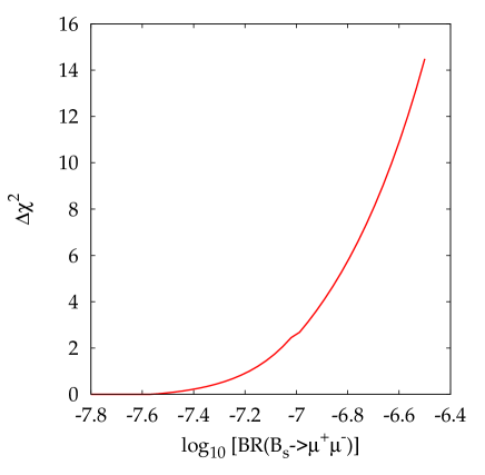
Figure 1: $\chi^{2}$ penalty on BR($B_{s}\rightarrow\mu^{+}\mu^{-}$) from [21]

The Tevatron has recently been instrumental in bounding the branching ratio of the rare decay channel $B_{s}\rightarrow\mu^{+}\mu^{-}$ [22]. Such bounds help constrain the mSUGRA parameter space [23]. We apply a $\chi^{2}$ penalty on the value predicted by micrOMEGAs1.3.6 derived from CDF Tevatron Run II data [21]. The resulting penalty is shown in Fig. 1.

Recently, it has been claimed that light sparticles are preferred by the two weak observables $\sin^{2}\theta_{w}^{l}$ and $M_{W}$ [4, 24]. In Ref. [9], $M_{W}$ and $\sin^{2}\theta_{w}^{l}$ were used at one loop order to help constrain mSUGRA in a global MCMC fit. The preference for such light SUSY was not particularly evident in the global fits. We examine the mSUGRA predictions for $M_{W}$ and $\sin^{2}\theta_{w}^{l}(\mbox{eff})$ in Figs. 3 and 3 for $A_{0}=0$, $\tan\beta=10$, $\mu>0$, equal $m_{0}$ and $M_{1/2}$ and central experimental values for the other inputs. For the “SOFTSUSY” lines, the default SOFTSUSY calculation is used. This contains the full SOFTSUSY MSSM contributions to the leptonic mixing angle $\sin^{2}\theta_{w}^{l}$ and $M_{W}$. It also contains the dominant 2-loop Standard Model contributions to $M_{W}$. For the lines marked “2-loop”, the SUSY Les Houches Accord is used to communicate with a currently private code that calculates the W-boson mass $M_{W}$ [10], and the effective leptonic mixing angle variable $\sin^{2}\theta^{l}_{w}$, calculated to two loops in the dominant MSSM parameters. We use the most general MSSM result for the full one-loop contributions. Besides all known corrections due to SUSY particles, the full SM contributions are also included in the predictions for $M_{W}$ and $\sin^{2}\theta^{l}_{w}$, leading to the currently most accurate predictions within the MSSM. The “SM” lines show the SM limit, where all corrections involving sparticles are dropped, i.e. the state-of-the-art SM results [25, 26] with $M_{H^{\mathrm{SM}}}=M_{h}$. They vary slightly with $m_{0}=M_{1/2}$ because the varying mSUGRA parameters produce different values of the Higgs boson mass $m_{h}$. The horizontal lines on the figures show the current $1\sigma$ experimental limits [27, 28]

$$M_{W}=80.392\pm 0.031\mbox{~{}GeV},\qquad\sin^{2}\theta_{w}^{l}=0.23153\pm 0.00020,$$ (4)

where we have added experimental and theoretical errors in quadrature.

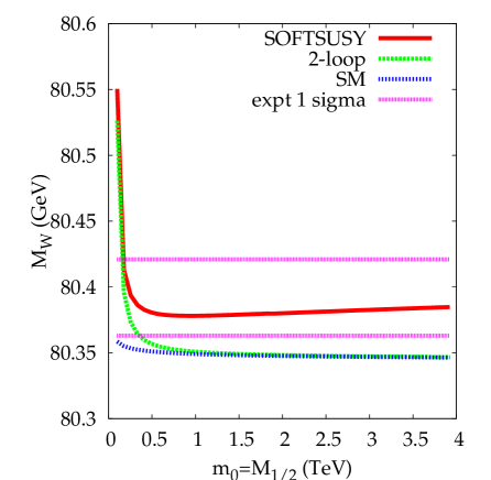
Figure 2: Various approximations to $M_{W}$ in mSUGRA

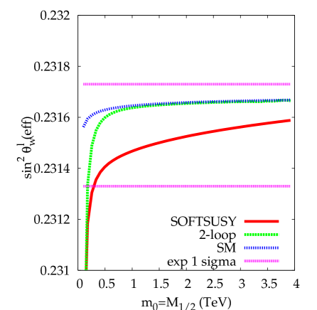
Figure 3: Various approximations to $\sin^{2}\theta_{w}$ in mSUGRA.

The theoretical errors in the predicted $M_{W}$ and $\sin^{2}\theta_{w}^{l}$ are estimated to be $10$ MeV and 12$\times 10^{-5}$ respectively [1]. We use these uncertainties for the purposes of comparison, although they have been slightly reduced recently by the addition of additional two-loop corrections taken into account in the present analysis [10, 29]. We see from the SOFTSUSY line in the figure that the prediction of $M_{W}$ does not have a strong preference for light SUSY, since the model is within the 1$\sigma$ errors up until $m_{0}=M_{1/2}=4$ TeV. In actual fact, only very light SUSY masses are disfavoured by the “SOFTSUSY” line, leading to predictions above the $1\sigma$-range. The situation is similar for the $\sin^{2}\theta^{l}_{w}$ “SOFTSUSY” line, where again only very light SUSY masses lead to predictions outside the $1\sigma$-range. However, using the best available predictions, corresponding to the “2-loop” lines, a preference for light $m_{0}=M_{1/2}$ can be seen in the prediction for $M_{W}$. The SM curve which lies just below the $1\sigma$-interval is approached from above in the decoupling limit, furthermore indicating a slight preference of the MSSM over the SM. The preference for light SUSY is not as striking for $\sin^{2}\theta_{w}^{l}$. Here most of the $m_{0}=M_{1/2}$ values are doing equally well, which is mainly due to the fact that the SM prediction for $\sin^{2}\theta_{w}^{l}$ is already well within the $1\sigma$-range. With the behaviour of the “one-loop” curve and the best available result being qualitatively different, it is desirable to use the more accurate result for $M_{W}$ and $\sin^{2}\theta_{w}^{l}$ when calculating the $\chi^{2}$ contributions of $M_{W}$ and $\sin^{2}\theta_{w}^{l}$ using Eq.1. Although Ref. [9] only used the one-loop predictions, the theoretical errors were correspondingly enlarged in order to take the larger uncertainty from higher order terms into account.

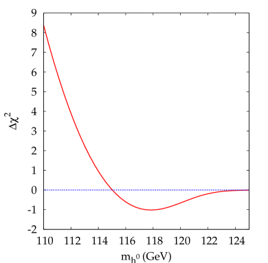
Figure 4: LEP2 higgs $\chi^{2}$ penalty paid

LEP2 constraints on the lightest CP-even higgs mass are included as a further likelihood penalty following a parameterisation of LEP2 data in the SM limit [30]. For the LEP2 constraints, the SM limit is a good approximation for mSUGRA, since sparticle mass limits imply that we must be near the decoupling régime of the MSSM [31]. We estimate that the SOFTSUSY2.0.7 determination of $m_{h}$ has a 2 GeV theoretical error in mSUGRA, although it may be somewhat larger in the general MSSM [32]. We therefore smear the parameterised LEP2 Higgs likelihood density ${\mathcal{L}}_{LEP2}(m_{h})$ with a Gaussian distribution of width $\sigma_{h}=2$ GeV:

$${\mathcal{L}}_{h}(m_{h})=\int_{m_{h}-4\sigma_{h}}^{m_{h}+4\sigma_{h}}dx\frac{1}{\sqrt{2\pi}\sigma_{h}}e^{\frac{-(m_{h}-x)^{2}}{2\sigma_{h}^{2}}}{\mathcal{L}}_{LEP2}(x).$$ (5)

The result of this procedure leads to the effective $\Delta\chi^{2}=-2\ln{\mathcal{L}}_{h}$ penalty shown in Fig. 4. The slight excess of candidate Higgs events over the background prediction at LEP2 can be seen by a negative $\Delta\chi^{2}$ penalty in the figure for $m_{h}\sim 116-121$ GeV.

The rare bottom quark branching ratio is $BR(b\rightarrow s\gamma)$ is constrained to be [33]

$$BR(b\rightarrow s\gamma)=(3.55\pm 0.38)\times 10^{-4},$$ (6)

obtained by adding the experimental error with the estimated theory error [34] of $0.3\times 10^{-4}$ in quadrature. Very recent estimates [35, 36] of $BR(b\rightarrow s\gamma)$ are compatible with Eq. 6 at the 1$\sigma$ level, although the error has decreased. Our prediction of $BR(b\rightarrow s\gamma)$ is substituted for $p_{i}$ in Eq. 1 in order to calculate $\chi_{BR(b\rightarrow s\gamma)}^{2}$.

We use the WMAP3 [37] power law $\Lambda$-CDM fitted value of

$$\Omega\equiv\Omega_{DM}h^{2}=0.104^{+0.0073}_{-0.0128}$$ (7)

for the dark matter relic density of the universe. We initially assume that the neutralinos are stable and that they constitute the whole of the dark matter relic density. Eq. 1 is used to calculate $\chi^{2}_{\Omega}$, with $\sigma_{\Omega}=0.0073$ for a prediction lower than the central experimental value and 0.0128 otherwise.

Having described the calculation of the likelihood associated with each individual measurement, we are now in a position to define the likelihood of the set of all measurements or observables, taken together. We are required to calculate the joint (total) likelihood $\mathcal{L}$ of all the measurements given the truth, i.e. in the notation of Eq 1 we want to know:

$${\mathcal{L}} = p(\mbox{measurements}|\mbox{true model})$$ (8)

$$= p(c_{1},c_{2},\ldots|{\bf m})$$ (9)

$$= p(c_{1}|{\bf m})\cdot p(c_{2}|c_{1},{\bf m})\cdot p(c_{3}|c_{1},c_{2},{\bf m})\cdot\ldots$$ (10)

$$= {\mathcal{L}}_{1}\cdot p(c_{2}|c_{1},{\bf m})\cdot p(c_{3}|c_{1},c_{2},{\bf m})\cdot\ldots$$ (11)

which is not in general equal to

$${\mathcal{L}}_{1}\cdot{\mathcal{L}}_{2}\cdot{\mathcal{L}}_{3}\cdot\ldots$$ (12)

unless we can be confident that for each measurement

$$p(c_{3}|c_{1},c_{2},{\bf m})\approx p(c_{3}|{\bf m})\mbox{\qquad{\em etc}}.$$ (13)

Fortunately we can be confident that Eq 13 does hold in our situation, as we have deliberately constructed ${\bf m}$ to be broad enough such that all fundamental parameters which might reasonably be expected to correlate any two of the measurements are included within it. We are therefore at liberty to write:

$${\mathcal{L}} = {\mathcal{L}}_{1}\cdot{\mathcal{L}}_{2}\cdot{\mathcal{L}}_{3}\cdot\ldots$$ (14)

$$= e^{-\sum_{i}\chi_{i}^{2}/2}$$ (15)

for the total likelihood, and we can be confident that this product takes into account the expected correlations between all the observables contained, due to the nature of the space $\left\{{\bf m}\right\}$ of models considered.

3 Dark Side Fits

Figure 5: mSUGRA Fits for (a) $\mu<0$ (b) $\mu>0$ marginalised to the $m_{0}$-$M_{1/2}$ plane. The posterior probability is indicated by the bar on the right hand side. The inner (outer) contours show the $68\%$ $(95\%)$ confidence region respectively.

We now compare and contrast the dark side fits to those with $\mu>0$. In Figs. 5(a) and 5(b), we show the posterior probabilities $P$ marginalised to the $m_{0}-M_{1/2}$ plane for both signs of $\mu$. As with all 2-dimensional marginalised plots in this paper, we bin the plane into 75$\times$75 2-dimensional bins. The colour bar on the right hand side of the figures shows the posterior probability $P$ of each bin divided by the maximum posterior probability of any bin in the plot. In Fig. 5(a), the only 68$\%$ contour is at the lowest values of $m_{0}$: all other contours are 95$\%$ confidence region contours due to the lowish likelihood densities. The brokenness of the contours is a result of statistical fluctuations in the results. Although these are visible, there is clearly reliable information their trajectories in the plot. The $\mu<0$ plot displays two isolated local maxima, whereas the 95$\%$ confidence region of $\mu>0$ is continuously connected. We discuss the relative normalisation of the two $\mu<0$ maxima in appendix B. In the 95$\%$ confidence region of Fig. 5a closest to the origin, the relic density is dominantly depleted by either stop co-annihilation [38, 39, 40] ${\tilde{t}}\chi_{1}^{0}\rightarrow tg$ or stau co-annihilation [41] ${\tilde{\tau}}_{1}\chi_{1}^{0}\rightarrow\tau\gamma$. On the other hand, the 95$\%$ region at higher $m_{0}-M_{1/2}$ consists of resonant Higgs annihilation regions [42, 43, 44], where $\chi_{1}^{0}\chi_{1}^{0}\rightarrow h,A^{0}\rightarrow b{\bar{b}}/\tau^{+}\tau^{-}$ and the focus point region where the LSP has a significant higgsino component and $\chi_{1}^{0}\chi_{1}^{0}\rightarrow ZZ,WW,t\bar{t}$ [45, 46, 47]. There was no significant stop co-annihilation [38, 39, 40] region for $\mu>0$.

Figure 6: Constraints from global fits with $\mu<0$ mSUGRA marginalised to 2-dimensional parameter planes. We have assumed a flat prior. The posterior probability is indicated by the bar on the right hand side. The inner (outer) contours show the boundary of a $68\%$ $(95\%)$ confidence region.

We now include some other marginalisations on the other 2-dimensional parameter planes for $\mu<0$ mSUGRA with a flat prior. They are displayed in Figs. 6(a)-(d). Figs. 6(a) and 6(b) show that the probability density for the 2-chain co-annihilation sample is not separated from the other sample in either the $M_{1/2}-A_{0}$ plane or the $\tan\beta$-$A_{0}$ plane (the almost disconnected region at the bottom of Fig. 6(a) consists of the light $h^{0}$-pole region). There is only a modest separation in the $M_{1/2}$-$\tan\beta$ plane: the 68$\%$ contours do not connect the two regions, whereas the 95$\%$ contours do. Fig. 6(d) shows that the connection between the two samples in the $m_{0}-\tan\beta$ plane is marginal. The $m_{0}-A_{0}$ marginalisation was useful for investigating the physics behind the two isolated probability maxima, and is displayed in appendix B.

Figure 7: Probability distributions in mass of (a) the lightest CP even higgs, (b) gluino, (c) the left-handed squark and (d) the neutralino. Flat priors have been assumed.

The probability distributions of the masses of selected MSSM particles are shown in Fig. 7 for both signs of $\mu$ in mSUGRA. The $\mu<0$ sample has not been normalised to the correct relative normalisation compared to $\mu>0$ in the figure. The lightest CP-even higgs, the gluino and the lightest neutralino all have mass distributions that are remarkably similar for either sign of $\mu$. However, in Fig. 7(c), we see that the $\mu<0$ sample has a flat plateau for higher squark masses, whereas the $\mu>0$ sample tails off somewhat. High squark masses will result in smaller total SUSY cross-sections at the LHC but the lighter gluino should still provide enough events for discovery if $m_{\tilde{g}}<2$ TeV [48, 49]. Sharp peaks at low gluino and neutralino masses are due to the $h^{0}$-resonance annihilation region [7]. The broader peak of the $\mu<0$ curve in Fig. 7(c) is due mostly to the co-annihilation sample. The significant probability densities for large gluino and squark masses are rather alarming, as then SUSY detection at the LHC would require a longer running time. Gauginos are not so sensitive to the range of the prior in Table 1 but the sfermions are [9] and a reduced range makes lighter sfermions more likely. Also, naturalness priors [8] have a large impact, reducing the likely sparticle masses.

3.1 Further investigations of the fits

We examine the best-fit points from each sampling in Table 3.

	$\mu<0$	$\mu>0$		$\mu<0$	$\mu>0$
$m_{0}$/GeV	3610	156	$\delta a_{\mu}/10^{-10}$	-0.4	14.2
$M_{1/2}$/GeV	93	569	$BR(b\rightarrow s\gamma)/10^{-4}$	3.65	3.41
$A_{0}$/GeV	-56	270	$BR(B_{s}\rightarrow\mu^{+}\mu^{-})/10^{-9}$	3.1	3.7
$\tan\beta$	6.0	24.1	$\sin^{2}\theta_{w}^{l}(\mbox{eff})$	0.23153	0.23152
$\Omega_{DM}h^{2}$	0.102	0.101	$M_{W}$/GeV	80.382	80.368
$m_{h}$/GeV	117.5	115.8	$\chi^{2}$	4.5	1.5

Table 3: Best-fit points from the MCMC samplings for each sign of $\mu$. $\chi^{2}\equiv\sum_{i}\chi_{i}^{2}$ and the Standard Model inputs are close to their experimental central values in each case.

We see from the table that, as expected, the $\mu>0$ sample has a better best-fit point and a correspondingly lower $\chi^{2}$, mainly due to the much better fit to $\delta a_{\mu}$. In agreement with Refs. [4, 24], the best-fit $\mu>0$ point is at light SUSY masses. The $m_{0}$ and $M_{1/2}$ parameters are smaller for the $\mu>0$ case than for $\mu<0$, corresponding to lighter sparticles and the larger contribution to the anomalous magnetic moment of the muon. If we take the $\mu<0$ best-fit point and flip the sign of $\mu$, we find that the point does not break electroweak symmetry properly and is excluded. The $\mu>0$ best-fit point has a total $\chi^{2}$ of 181 when the sign of $\mu$ is flipped, mostly due to an increase in the predicted value of $\Omega_{DM}h^{2}$ to 0.195.

The region of smaller $m_{0}$, $M_{1/2}$ is more probable for $\mu>0$ than for $\mu<0$: this will lead to a relatively heavier $\mu<0$ spectrum. Our $\mu>0$ results are generally similar to previous analyses which did not include $M_{W}$ and $\sin^{2}\theta_{w}^{l}$ as constraints in Ref. [7] and to those which included the one-loop SOFTSUSY prediction for $M_{W}$, $\sin^{2}\theta_{w}^{l}$ with enlarged theoretical errors [9]. This seems in contradiction to the conclusions of Ellis et al [4, 24], where it is claimed that the electroweak variables prefer light SUSY. Indeed, Fig. 3 indicates that $M_{W}$, $\sin^{2}\theta_{w}^{l}$ do mildly prefer light SUSY but our results show that this preference is washed out in the global fits. Our results allow for heavier sparticles than Ellis et al, mainly because we have chosen to allow more relevant parameters to vary: 8 compared to 2 in their paper (one dimension is fixed by requiring the relic density prediction to be the central WMAP-constrained value). Their fits are for different discrete values of fixed $\tan\beta$, but if it were allowed to vary, we believe that the confidence regions there would be enlarged. In the present paper, we also obtain additional smearing from allowing $m_{t}$, $\alpha_{s}$, $\alpha$ and $m_{b}$ to vary.

Figure 8: Posterior probability distributions for weak observables in mSUGRA.

Figs. 8(a) and 8(b) show the probability distributions for $M_{W}$, $\sin^{2}\theta_{w}^{l}$ coming from the mSUGRA fits for both signs of $\mu$, although the sign does not make much difference. We see that the $M_{W}$ prediction coming from the fits is skewed towards values lower than the central empirical value, corresponding to a preference for heavy SUSY from the rest of the fits. Fig. 3 confirms that heavier SUSY tends to have lighter values of $M_{W}$. From Fig. 3, we see that heavy SUSY tends to be on the upper 1$\sigma$ empirical limit of $\sin^{2}\theta_{w}^{l}$. Fig. 8(b) does show evidence for this skew, which is rather mild.

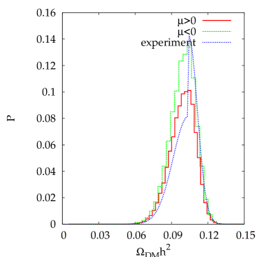
Figure 9: Dark matter relic density probability distribution

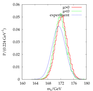
Figure 10: Top mass probability distribution

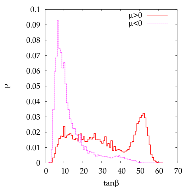
Figure 11: Probability distribution for $\tan\beta$ in mSUGRA

The strongest constraint in the fits comes from the dark matter relic density. In Fig. 10, we show the probability densities resulting from the fits for the dark matter relic density. Each curve is normalised slightly differently to allow better viewing of the results. We see that both the $\mu>0$ and the $\mu<0$ $\Omega_{DM}h^{2}$ distributions follow the empirical constraint closely, except for a slight excess just lower than the central value.

Another important aspect influencing the fits is the integrated volume of the probability density, which is automatically taken into account in a Bayesian analysis, as was demonstrated and pointed out in Ref. [9]. The usual arguments based purely on values of $\chi^{2}$ above the best-fit value are valid when the probability density function is Gaussian in the interesting parameters (which is certainly not the case here, as even a cursory glance at Fig. 5 allows). Thus even if, say, the stop co-annihilation region had a much lower $\chi^{2}$ than other regions of the fits, the fact that its volume in 8-dimensional input parameter space is much smaller than the other regions will automatically disfavour it since its integrated probability will be low.

The LEP2 higgs constraints shown in Fig. 4, along with the current empirical value of $m_{t}$ shown in Table 1 favours rather heavy mSUGRA. Indeed, Fig. 10 shows that $m_{t}$ is skewed to somewhat higher masses than the empirical constraint, illustrating this tension (again, we have altered the normalisation of the curves slightly for clarity). Inspection of the $\alpha(M_{Z})^{\overline{MS}}$, $\alpha_{s}(M_{Z})^{\overline{MS}}$, $m_{b}(m_{b})$ inputs show that they follow their empirical probability distributions very closely. There is a large volume of parameter space for the $A^{0}$ dark matter annihilation region at high $\tan\beta>10$ particularly for $\mu>0$, as shown in Fig. 11. High values of $\tan\beta$ mean that light SUSY is disfavoured by $BR[b\rightarrow s\gamma]$ and $BR[B_{s}\rightarrow\mu^{+}\mu^{-}]$ since the data disfavours SUSY contributions [23], which are approximately proportional to $\tan^{2}\beta/M_{SUSY}^{4}$ and $\tan^{6}\beta/M_{SUSY}^{4}$ respectively. The distributions of these two observables are shown in Fig. 12. As can be seen from the figure, the sign of the SUSY contribution to each observable depends upon the sign of $\mu$. The maxima in each figure correspond to observables being close to their SM limit. $BR[b\rightarrow s\gamma]$ prefers $\mu>0$ mildly, as $\mu<0$ tends to predict a $BR[b\rightarrow s\gamma]$ larger than the central empirical value.

Figure 12: Probability distributions of (a) $BR(b\rightarrow s\gamma)$ and (b)$BR(B_{s}\rightarrow\mu^{+}\mu^{-})$ in mSUGRA.

Figure 13: Probability distributions for $\delta a_{\mu}$ in mSUGRA (a) for flat priors and both signs of $\mu$ and (b) for $\mu>0$ and various different priors. The key is explained in the text.

$(g-2)_{\mu}$ is expected to be the observable that most strongly discriminates between the two signs of $\mu$. We plot its distribution in each case in Fig. 13(a). Since $\mu<0$ has the wrong sign of $\delta a_{\mu}$ compared to experiment, the probability density bunches around zero. Clearly heavy SUSY with a less negative SUSY contribution is favoured. However, we see that the $\mu>0$ distribution also prefers smaller SUSY contributions than the data in the global fits. This was initially unexpected, and will lead to $\mu<0$ mSUGRA being less ruled out. In order to understand this behaviour better, we re-weight the $\mu>0$ sample in various ways. $\delta a_{\mu}$ is approximately proportional to $\tan^{2}\beta/M_{SUSY}^{4}$ and we need large $\tan\beta$ and rather light SUSY in order to get a sizable value in line with the central experimental value. As explained above, this is somewhat in conflict with LEP2 Higgs constraints and $BR(b\rightarrow s\gamma)$. We re-weight the $\mu>0$ chains, dividing by a number that removes the likelihood contribution from the LEP2 Higgs constraint and the $BR(b\rightarrow s\gamma)$ measurement, i.e. ${\mathcal{L}}_{h}{\mathcal{L}}_{BR(b\rightarrow s\gamma)}$. The probability distribution of $\delta a_{\mu}$ resulting from this procedure is marked as the “reduced” curve in Fig. 13(b). It extends to somewhat higher and more central values of $\delta a_{\mu}$, showing that some of the skew in the $\delta a_{\mu}$ distribution does come from the LEP2 Higgs and $BR(b\rightarrow s\gamma)$ measurements. However, the effect is rather small and the resulting distribution is rather far from the experimental distribution, indicating a further effect. There could be a significant volume effect if regions of parameter space that have central values of $\delta a_{\mu}$ have a small volume. This would render our results sensitive to the prior, since by changing the measure of the input parameters, we can change the volume measure [8]. In order to investigate the effects of this, we re-weight the $\mu>0$ chains by a factor $1/(m_{0}M_{1/2})$. Such a re-weighting mimics the effect of using a logarithmic prior on $m_{0}$ and $M_{1/2}$ since

$$\int P(m_{0},M_{1/2})\ d\ln m_{0}\ d\ln M_{1/2} = \int P(m_{0},M_{1/2})\frac{d\ln m_{0}}{dm_{0}}\frac{d\ln M_{1/2}}{dM_{1/2}}\ dm_{0}\ dM_{1/2}$$ (16)

$$= \int\left(\frac{P(m_{0},M_{1/2})}{m_{0}M_{1/2}}\right)\ dm_{0}\ dM_{1/2}.$$

One might consider such a prior on technical naturalness grounds. The “log prior” results are displayed in Fig. 13(b). They have a fatter tail out to higher values of $\delta a_{\mu}$ than the flat prior sample or the “reduced” sample. When we perform the re-weighting in Eq. 16 as well as the one to remove $BR(b\rightarrow s\gamma)$ and LEP2 Higgs constraints, we obtain the “log prior, reduced” curve in the figure. This shows a yet fatter tail and is starting to approach the empirical probability distribution imposed on the fits. Our results are obviously somewhat dependent upon the prior. This is essentially because there is not enough precise data yet to constrain mSUGRA very strongly. We must bear in mind this dependence upon the prior, and investigate different priors when we estimate $P_{-}/P_{+}$ below.

prior	flat	small	log
$P_{-}/P_{+}$	0.16	0.12	0.07

Table 4: Ratios of integrated probability for different signs of $\mu$.

The total normalisation of the $\mu>0$, $\mu<0$ samples is shown in Table 4 for various different priors. The “small” prior is a flat prior with a reduced range compared to the one displayed in Table 1. We filter the chains to only include points with $m_{0}<2$ TeV and $|A_{0}|<2$ TeV. The table shows that $\mu<0$ is somewhat disfavoured for the smaller ranges and more disfavoured still for the log prior. The result is somewhat sensitive to the prior, indicating the need for more data. We therefore prefer to quote a range for $P_{-}/P_{+}=0.07-0.16$ depending upon the prior. This range is a focal result of the present paper.

4 Fits Without WMAP3

Figure 14: Constraints from global fits without the dark matter constraint with (a) $\mu>0$ and (b) $\mu<0$ mSUGRA marginalised to the $m_{0}$-$M_{1/2}$ plane. We have assumed a flat prior. The posterior probability is indicated by the bar on the right hand side. The inner (outer) contours show the boundary of a $68\%$ $(95\%)$ confidence region.

We now briefly examine the effect of removing the dark matter $\chi^{2}$ penalty from the fits. We could in principle re-weight the chains in order to do this, but we find that that leads to statistical fluctuations in the results that are too large. Initial investigations revealed that the efficiency becomes much higher when we remove the dark matter relic density contribution to the total $\chi^{2}$. We are able to increase the widths of the proposal distribution to 197 GeV for $m_{0}$, 100 GeV for $M_{1/2}$, 400 GeV for $A_{0}$, 8.5 for $\tan\beta$ and 1$\sigma$ for the Standard Model inputs and still achieve an efficiency of around 35$\%$. This has the consequence that the chains explore the parameter space much quicker than in the previous section, and so less MCMC steps are needed. We run a further 9$\times$200 000 MCMC steps for each sign of $\mu$. This time, both signs of $\mu$ have excellent convergence statistics, $\hat{R}$ being different to 1 at the per-mille level only in each case.

Figure 15: Probability distributions in mass of (a) the lightest CP even higgs, (b) gluino, (c) the left-handed squark and (d) the neutralino. Flat priors have been assumed.

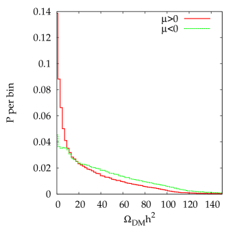
Figure 16: $\Omega h^{2}$ distributions without imposing the dark matter constraint.

We see from Fig. 14 that removing the dark matter constraint yields a very different picture for the mSUGRA probability distributions in the $m_{0}$-$M_{1/2}$ plane. This confirms our statement that many of the features seen in the previous section are due precisely to that constraint. The probability distribution is now much flatter in the input parameter space. The disallowed region at low $m_{0}$ and high $M_{1/2}$ is due to the no-charged LSP constraint. The disallowed region at low $m_{0}$ and low $M_{1/2}$ is due mostly to the combined effect of the $(g-2)_{\mu}$, $BR(b\rightarrow s\gamma)$ and $m_{h}$ constraints. The disallowed region is significantly larger for $\mu<0$ than for $\mu>0$, due to those three observables. Marginalisations in other mSUGRA input parameter planes tell a similar story, more featureless than the fits including the dark matter constraint. As mentioned in the introduction, Fig. 14 covers the case of R-parity violating mSUGRA when the R-parity violating couplings are smaller than about 0.1. For larger R-parity violating couplings, one would have to include them in the renormalisation group equations to obtain accurate results.

The more featureless fits have predictable effects on the mass spectrum of the MSSM, as shown in Fig. 15. We have fixed the ranges of the abscissas to be identical to those in Fig. 7 in order to facilitate comparison. The lightest CP-even Higgs probability distribution is broader and shifted to heavier values, due to the bigger volume of parameter space allowed at higher $m_{0}$ and $M_{1/2}$ values. Gluino mass distributions no longer tail off at higher masses: upper bounds would be mostly determined by the cut-off placed $m_{0}$ and $M_{1/2}$. The gluino mass and neutralino distributions are also much less peaked than the ones in Figs. 7b,d particularly for $\mu<0$. The flatter distributions are, of course, an indication that the data aren’t strongly constraining. Large volumes at large $m_{0},M_{1/2}$ effectively move up the squark masses, as Fig. 15c illustrates.

The probability distribution of $\Omega_{DM}h^{2}$ is shown in Fig. 16 for each sign of $\mu$, when we drop the relic dark matter $\chi^{2}$ contribution. In the figure, we see that huge values can result: in fact the mean value for the $\mu>0$ sample tails off at $\Omega_{DM}h^{2}\sim 128$, much larger than the WMAP3 value of 0.1.

prior	flat	small	log
${P_{-}/P_{+}}$	0.45	0.43	0.19

Table 5: Ratios of integrated probability for different signs of $\mu$ with no dark matter constraint.

This illustrates the fact that regions of parameter space which fit the dark matter data in mSUGRA need some special annihilation mechanism that is not typical of the whole space. This and similar arguments have led several authors to consider non-universal models [50, 51], where the relic density might be less fine-tuned. The distributions are highly skewed, having tiny tails up to $\Omega h^{2}\sim 1000$. The relative normalisation of $\mu>0$ to $\mu<0$ is calculated in the same manner as in the previous section for different priors, and displayed in Table 5. $\mu<0$ is hardly disfavoured in R-parity violating mSUGRA (where we can neglect the dark matter constraint), where $P_{-}/P_{+}=0.19-0.45$.

5 Conclusions

We have performed global fits to mSUGRA using indirect data and state-of-the-art predictions of the observables. The MCMC technique was successfully employed despite initial non-convergence of the $\mu<0$ chains. Bridge sampling was used to normalise two isolated maxima that had not been traversed by any chain for $\mu<0$. We found that $\mu<0$ is somewhat disfavoured in comparison to $\mu>0$ but not by huge margins. The rest of the fit prefers rather heavy SUSY and so the SUSY contribution to $(g-2)_{\mu}$ is small whichever the sign of $\mu$. $\mu<0$ is only disfavoured marginally, the ratio of integrated probability densities being $P_{-}/P_{+}=0.07-0.16$ depending upon the prior. We see from Fig. 16 that without the dark matter constraint, $\Omega_{DM}h^{2}$ is predicted up to values of around 128. This corresponds to a $\chi^{2}_{\Omega}$ of around 3$\times 10^{8}$, much larger than is likely from the other observables such as $M_{W}$ or $\sin^{2}\theta_{w}^{l}(\mbox{eff})$. The fits are therefore completely dominated by the dark matter relic density constraint and volume effects. Expectations that the SUSY scale will be light because of a preference from weak observables turn out not to be true in the global fits. If the dark matter constraint is dropped, as would be the case for R-parity violation, $\mu<0$ is hardly disfavoured at all, $P_{-}/P_{+}=0.19-0.45$. $\mu<0$ is much less disfavoured than many seem to assume. Many recent analyses only consider $\mu>0$ on the grounds that $\mu<0$ is strongly disfavoured by $(g-2)_{\mu}$. We have therefore demonstrated that this is not the case when one considers the entirety of the data and that $\mu<0$ should still be considered in mSUGRA analyses.

It could be argued that the flat measure used here in $m_{0}$, $M_{1/2}$, $A_{0}$ and $\tan\beta$ can be improved upon. For instance, $\tan\beta$ is really a derived quantity and is related to more fundamental Higgs potential parameters, which could be considered more natural to have a flat measure upon. There is also the issue of fine-tuning, recently illuminated in Ref. [52]: we could disfavour regions of parameter space that are highly fine-tuned, for instance [8]. Changes such as these in the prior could potentially change the results of the fits and we intend to investigate them in a future publication.

Clearly, more data is required to decrease the dependence of results on the prior. The most helpful data is likely to be that from colliders. The MCMC fitting technique has been used in an ATLAS study examining how cross-section and kinematic endpoint information constrains mSUGRA and non-universal models [53]. At this moment, without data from colliders, we are forced to use indirect constraints for the observables. However, in the future it will be desirable to predict $\Omega_{DM}h^{2}$ given some SUSY collider observables [54, 55]. If this is in contradiction with the observed value from cosmology, it will point to a wrong cosmological assumption, which could then be changed. In order to really confirm that dark matter particles have been produced at colliders, one requires compatibility with direct dark matter detection data. Of course one would like to drop the mSUGRA assumption and perform a general SUSY analysis, but for this it is likely that additional data from a future international linear collider would be required [54, 55]. In any case, the techniques investigated in this paper should prove useful for the fits.

Appendix A Markov Chain Monte Carlos

Our Markov chain consists of a list of parameter points (${\mathbf{x}}^{(t)}$) and associated likelihood densities (${\mathcal{L}}({\mathbf{x}}^{(t)})$). Here, $t$ labels the link number in the chain. Given some point at the end of the Markov chain (${\mathbf{x}}^{(t)}$), the Metropolis-Hastings algorithm [56, 57, 58] requires one to randomly pick another potential point (${\mathbf{x}}$) (typically in the vicinity of ${\mathbf{x}}^{(t)}$) using a proposal distribution $Q({\mathbf{x}};{\mathbf{x}}^{(t)})$. There is a large amount of freedom in the choice of the proposal function $Q$, and this freedom is usually exploited to improve the efficiency of the sampling process. In order to ensure that the choice of $Q$ does not bias the final set of samples in some way, the form of $Q$ is taken into account when deciding whether to accept or reject the new point. If the ratio $\rho$ defined by

$$\rho=\frac{{\mathcal{L}}({\bf x})}{{\mathcal{L}}{({\bf x}^{(t)})}}\frac{Q({\mathbf{x}}^{(t)};{\mathbf{x}})}{Q({\mathbf{x}};{\mathbf{x}}^{(t)})}$$ (17)

is greater than one, the new point ${\bf x}$ is appended to the chain. If $\rho$ is instead less than one, a decision must be made to determine whether to accept or reject the proposed point ${\bf x}$. The rule is that acceptance of ${\bf x}$ must occur with probability $\rho$. If accepted, ${\bf x}$ is added to the end of the chain. If not accepted, the point ${\mathbf{x}}^{(t)}$ is copied once more onto the end of the chain. Whichever point makes it on to the end of the chain is thereafter known as ${\mathbf{x}}^{(t+1)}$.

As a result of following the above steps, the sampling density of points in the chain becomes proportional to the density of the target distribution (such as the posterior probability density, or the likelihood when the prior is uniform) as the number of links goes to infinity, under the circumstances described in Ref. [58]. The Metropolis-Hastings MCMC algorithm is typically much more efficient than a straightforward scan for the dimensionality of input parameter space $D>3$; the number of required steps scales roughly linearly with $D$ rather than as a power law. We take the proposal function $Q$ to be a product of Gaussian distributions along each dimension $k=1,2,\ldots,D$ centred on the location of the current point along that dimension, i.e. $x^{(t)}_{k}$:

$$Q({\mathbf{x}};{\mathbf{x}}^{(t)})=\prod_{k=1}^{D}\frac{1}{\sqrt{2\pi}l_{k}}e^{-(x_{k}-x_{k}^{(t)})^{2}/2l_{k}^{2}},$$ (18)

where $l_{k}$ denotes the width of the distribution along direction $k$. For the case where we include the dark matter relic density in the calculation, we choose $l_{m_{0}}=100$ GeV, $l_{M_{1/2}}=50$ GeV, $l_{A_{0}}=400$ GeV and $l_{\tan\beta}=3$. For the Standard Model inputs, we choose $l_{k}=8\sigma_{k}/20$. We discuss why these particular values were chosen in the next section.

In order to start the chain we follow the following procedure, which finds a point at random in parameter space that is not a terrible fit to the data. We pick some ${\mathbf{y}}^{(0)}$ at random in the mSUGRA parameter space using a flat distribution for its probability density function (pdf). The Markov chain for ${\mathbf{y}}$ is evolved through 2000 steps. We then set ${\mathbf{x}}^{(0)}={\mathbf{y}}^{(2000)}$, continuing the Markov chain in ${\mathbf{x}}$ and discarding the “burn-in” chain ${\mathbf{y}}$. A reasonable-fit point is typically found long before 2000 iterations of the Markov chain. We must make sure that we perform enough iterations after this point that the chain traverses the remaining viable parameter space. We will provide a convergence test to this effect.

A.1 Efficiency

The efficiency of a chain can be defined as “the number of links whose coordinates differ from those of their predecessor in the chain” divided by “the total number of points in the chain”. There will always be a tension between efficiency and convergence in chains: if the $l_{k}$ are set to be too small, efficiency will increase but the chain will take too long to achieve convergence whereas if they are too large, the efficiency will be so small that the sampling will contain large statistical fluctuations. In practice, the bulk of our posterior probability density is contained in a very thin hyper-surface in the 8-dimensional input parameter space [7]. It is thin because $\Omega_{DM}h^{2}$ varies very rapidly over mSUGRA space compared to the high accuracy of the empirical constraint. With the $l_{k}$ listed above, we found that efficiencies were at the per-mille level, too small to achieve a statistically stable result in a reasonable amount of CPU time. To achieve a significantly larger efficiency, we had to reduce $l_{k}$ to such a level that we lost convergence because the chains had not traversed the viable parameter space. In order to counter this, we expanded the errors on $\Omega_{DM}h^{2}$ to $\pm 0.02$ while calculating the likelihood density in the chain. This artificially thickens the “surface” containing the bulk of the posterior probability density, increasing the efficiency to much more reasonable values of around 5–7$\%$. In order to correct for this artificial thickening and re-impose the required constraint of Eq. 7, it was therefore necessary to re-weight each link of each chain at the end of the sampling. Each link is re-weighted by the ratio of the proper likelihood density ${\mathcal{L}}_{P}$ to the likelihood density with inflated errors ${\mathcal{L}}_{I}$:

$$\frac{{\mathcal{L}}_{P}}{{\mathcal{L}}_{I}}=\exp\left({-\frac{(c_{\Omega}-p_{\Omega})^{2}}{2\sigma^{2}_{\Omega}}}\right)\div\exp\left(-\frac{(c_{\Omega}-p_{\Omega})^{2}}{2\times 0.02^{2}}\right)$$ (19)

in order to impose the correct penalty on the links. We ignore additional constants that are independent of $\Omega_{DM}h^{2}$ in this expression since the overall normalisation of the likelihood density is here undetermined. The re-weighting procedure necessarily degrades the statistical spread of the results, however we find that the increase in efficiency more than compensates for this effect. Below, we re-weight different variables in order to investigate various features in the results, but the method remains analogous to the one described here.

A.2 Bridge Sampling

One of the numbers we will require from our MCMC samples is the ratio of integrated posterior probabilities of $\mu>0$ ($P_{+}$) and $\mu<0$ ($P_{-}$). This ratio will tell us the extent to which $\mu<0$ is disfavoured over $\mu>0$. Assuming a flat prior in the variables of the model, the posterior probability is equal to the integrated likelihood divided by a factor which does not depend upon model hypotheses or parameters. Thus $P_{-}/P_{+}=\int d{\bf x}{\mathcal{L}}_{-}({\bf x})/\int d{\bf x}{\mathcal{L}}_{+}({\bf x})$, where ${\mathcal{L}}_{+,-}({\bf x})$ is the likelihood density of $\mu>0$ $(<0)$ mSUGRA respectively at parameter point $({\bf x})$. One way to estimate this ratio would be to include the sign of $\mu$ as a free parameter in the Metropolis-Hastings procedure, to be chosen randomly in a proposal point. This algorithm leads to large inefficiencies because the $\mu>0$ and $\mu<0$ likelihood surfaces have a limited overlap, meaning that too many proposals for an opposite sign of $\mu$ will be rejected. Also, the procedure would likely provide large statistical fluctuations for the disfavoured sample, which we expect to be the $\mu<0$ one. Even though it is disfavoured, we should like to investigate its properties.

A simple way one might hope to evaluate the ratio ${P_{-}}/{P_{+}}$ is

$$\frac{P_{-}}{P_{+}}=\frac{1}{E_{-}\left[\frac{{\mathcal{L}}_{+}}{{\mathcal{L}}_{-}}\right]}\approx\frac{1}{N}\sum_{t=1}^{N}\frac{{\mathcal{L}}_{-}({\mathbf{x}_{i}^{(t)}})}{{\mathcal{L}}_{+}({\mathbf{x}_{i}^{(t)}})},$$ (20)

where $E_{-}$ denotes the expectation with respect to the $\mu<0$ likelihood distribution [12]. $N$ denotes the number of MCMC steps. Unfortunately, a simple importance sampling estimate of this kind does not work if there are any valid points (${\mathcal{L}}\neq 0$) for one sign of $\mu$ that are invalid (${\mathcal{L}}=0$) for the opposite sign of $\mu$. In our case there are plenty of these dangerous pairings, as sparticle mass or tachyonic bounds move around in parameter space depending upon the sign of $\mu$. To get around this problem, we use a solution known as bridge sampling [12] with a “geometric bridge”. This allows us to generate a (biased) estimator $r$ for the ratio ${P_{-}}/{P_{+}}$ as long as there is some viable region of $\mu>0$ parameter space that is also viable for $\mu<0$. The estimator for the ratio is constructed as follows:

$$\frac{P_{-}}{P_{+}}=\frac{E_{+}\left[\sqrt{\frac{{\mathcal{L}}_{-}}{{\mathcal{L}}_{+}}}\right]}{E_{-}\left[\sqrt{\frac{{\mathcal{L}}_{+}}{{\mathcal{L}}_{-}}}\right]}\approx r\equiv\frac{\sum_{t=1}^{N}\sqrt{\frac{{\mathcal{L}}_{-}({\mathbf{x}}_{+}^{(t)})}{{\mathcal{L}}_{+}({\mathbf{x}}_{+}^{(t)})}}}{\sum_{t=1}^{N}\sqrt{\frac{{\mathcal{L}}_{+}({\mathbf{x}}_{-}^{(t)})}{{\mathcal{L}}_{-}({\mathbf{x}}_{-}^{(t)})}}},$$ (21)

where $(\mathbf{x})^{(t)}_{+,-}$ are the parameter points of the links in the $\mu>0$ or $\mu<0$ chains respectively. Here, we have assumed an equal number of links in each chain. In summary, to calculate $r$, we must run two chains, one for positive $\mu$ and one for negative $\mu$, and for every link, record the likelihood one would have obtained for identical input parameters except for the opposite sign of $\mu$.

Appendix B Convergence and Normalisation

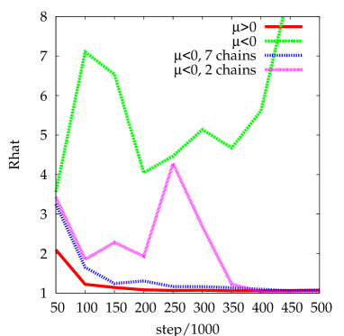
Figure 17: Convergence statistics for the MCMCs.

In order to evaluate the convergence of the MCMC chains, we always run 9 independent chains with different random starting points. By comparing the similarity of the resulting sampling densities of input parameters in the chains, one can construct [59] a measure of convergence $\hat{R}$. $\hat{R}$ is an upper bound on the reduction in variance of parameters that would result from running the chains for an infinite number of steps. The precise implementation is listed in Ref. [7]. Values close to 1 indicate convergence of the chains.

Figure 18: The two types of negative $\mu$ samples: (a) the “$\mu<0$, 2 chains” samples (later shown to be co-annihilation samples), and (b) the “$\mu<0$, 7 chains” samples (later shown to be non co-annihilation samples, dominated by resonant Higgs annihilation regions). The posterior probability is indicated by the bar on the right hand side. The inner (outer) contours show the boundary of a $68\%$ $(95\%)$ confidence region.

We run 9 chains of 500 000 points for $\mu>0$ mSUGRA and for the $\mu<0$ dark side of mSUGRA. The $\mu>0$ curve in Fig. 17 shows good convergence is achieved by 500 000 MCMC steps. However, the $\mu<0$ curve shows a problem: convergence is never achieved. This is a serious difficulty as one could not draw any quantitative statistical inferences from the non-converged chains. Further inspection of the $\mu<0$ results shows that two of the $\mu<0$ chains are in a completely different part of parameter space than the other seven. This indicates isolated maxima of likelihood density which the MCMC has not been able to jump between in the finite number of MCMC steps attempted. There is no balance between the two isolated maxima in the sample. Isolating the two anomalous $\mu<0$ chains and calculating $\hat{R}$ between just them, we obtain the “$\mu<0$, 2 chains” curve, which closely approaches 1 by 500 000 MCMC steps. Thus within this isolated maximum, convergence is achieved. The same can be said of the other “$\mu<0$, 7 chains” samples: they also converge amongst themselves. Thus, the shapes of each isolated maximum are well determined, but the relative normalisation of the two different types of negative $\mu$ samples is not.

Figure 19: Probability density in the lightest stop-lightest neutralino mass plane for the 2-chain sample. The posterior probability is indicated by the bar on the right hand side. The inner (outer) contours show the boundary of a $68\%$ $(95\%)$ confidence region.

In order to illustrate the two maxima, we marginalise the two types of negative $\mu$ samples onto the $m_{0}-A_{0}$ plane in Figs. 18(a) and 18(b). The maxima are isolated in this plane (as well as in some other 2-parameter planes). The two regions are completely separated. Their shape is primarily determined by regions which efficiently deplete the relic density of neutralinos which, in mSUGRA, is often higher than the WMAP3 constraint. We investigate the 2-chain sample in Fig. 19. In the figure, there are two good-fit regions: where the stau co-annihilates [41] (at moderate values of $A_{0}$, higher values of $m_{\tilde{t}}$ in the figure) with the LSP ${\tilde{\tau}}_{1}\chi_{1}^{0}\rightarrow\tau\gamma$ and where the lightest stop co-annihilates (at $A_{0}<-3$ TeV) with the LSP ${\tilde{t}}\chi_{1}^{0}\rightarrow tg$ in the early universe, where $m_{\chi_{1}^{0}}\approx m_{{\tilde{t}}_{1}}$, the lower strip in the figure. There was no significant stop co-annihilation [38, 39, 40] region for $\mu>0$. On the other hand, Fig. 18(b) dominantly consists of resonant Higgs annihilation regions [42, 43, 44], where $\chi_{1}^{0}\chi_{1}^{0}\rightarrow h,A^{0}\rightarrow b{\bar{b}}/\tau^{+}\tau^{-}$ and the focus point region where the LSP has a significant higgsino component and $\chi_{1}^{0}\chi_{1}^{0}\rightarrow ZZ,WW,t\bar{t}$ [45, 46, 47].

We need a method to determine the relative normalisation of the 2-chain co-annihilation sample and the 7-chain resonant higgs annihilation sample. Equivalently we need a method to determine the ratio of the posterior probability ${\tilde{P}}_{-}^{\tilde{t}}$ of the 2-chain co-annihilation sample and the posterior probability ${\tilde{P}}_{-}^{/\!\!\!{\tilde{t}}}$ of the 7-chain resonant higgs annihilation sample. We use ${\tilde{P}}$ to denote the fact that the posterior probabilities are un-normalised. Fortunately, Eq. 21 provides us with a solution: we first determine the normalisation of the $\mu>0$ sample with respect to each separate $\mu<0$ sample, i.e. ${\tilde{P}}_{-}^{\tilde{t}}/P_{+}$ and ${\tilde{P}}_{-}^{/\!\!\!{\tilde{t}}}/P_{+}$. Since these quantities individually have good convergence properties, their ratio is also well determined:

$$\frac{{\tilde{P}}_{-}^{/\!\!\!{\tilde{t}}}}{{\tilde{P}}_{-}^{\tilde{t}}}=\frac{{\tilde{P}}_{-}^{/\!\!\!{\tilde{t}}}}{P_{+}}\div\frac{{\tilde{P}}_{-}^{\tilde{t}}}{P_{+}}=0.097\div 0.063=1.53.$$ (22)

Normalising the probabilities as $a{\tilde{P}}_{-}^{{\tilde{t}}}\equiv P_{-}^{{\tilde{t}}}$, $b{\tilde{P}}_{-}^{/\!\!\!{\tilde{t}}}\equiv P_{-}^{/\!\!\!{\tilde{t}}}$, we fix $a$ and $b$ by imposing ${P}_{-}^{{\tilde{t}}}+{P}_{-}^{/\!\!\!{\tilde{t}}}=1$ and Eq. 22. The relative posterior probabilities ratios are re-calculated whenever alternative priors are investigated. In section 3 where we present the total $\mu<0$ sample results, we present posterior probability densities with the correct normalisation, according to this prescription. The ratio of the probability of $\mu<0$ to $\mu>0$ is then determined simply by:

$$\frac{P_{-}}{P_{+}}=\frac{P_{-}^{\tilde{t}}}{P_{+}}+\frac{P_{-}^{/\!\!\!{\tilde{t}}}}{P_{+}}.$$ (23)

It is worth noting that, had we been unlucky, we might have obtained only chains like those in the 7-chain sample. In that case we would have carried on with the analysis without realising about the different 2-chain sample, therefore any results achieved would have been incomplete. An obvious question is: were there any other local maxima that we have missed by not running enough chains? Unfortunately, any fitting procedure is susceptible to this caveat and there is no satisfactory answer. Finding a high but very narrow global maximum is an unsolved problem in any number of dimensions.

References

- [1] J. R. Ellis, K. A. Olive, Y. Santoso and V. C. Spanos, Likelihood analysis of the CMSSM parameter space, Phys. Rev. D 69 (2004) 095004 [arXiv:hep-ph/0310356].
- [2] S. Profumo and C. E. Yaguna, A statistical analysis of supersymmetric dark matter in the MSSM after WMAP, Phys. Rev. D 70 (2004) 095004 [arXiv:hep-ph/0407036].
- [3] E. A. Baltz and P. Gondolo, Markov chain Monte Carlo exploration of minimal supergravity with implications for dark matter, JHEP 0410 (2004) 052 [arXiv:hep-ph/0407039].
- [4] J. R. Ellis, S. Heinemeyer, K. A. Olive and G. Weiglein, Indirect sensitivities to the scale of supersymmetry, JHEP 0502 (2005) 013 [arXiv:hep-ph/0411216].
- [5] L. S. Stark, P. Hafliger, A. Biland and F. Pauss, New allowed mSUGRA parameter space from variations of the trilinear scalar coupling A0, JHEP 0508 (2005) 059 [arXiv:hep-ph/0502197].
- [6] R. G. Roberts and L. Roszkowski, Implications for minimal supersymmetry from grand unification and the neutrino relic abundance, Phys. Lett. B 309 (1993) 329 [arXiv:hep-ph/9301267].
- [7] B. C. Allanach and C. G. Lester, Multi-dimensional mSUGRA likelihood maps, Phys. Rev. D 73 (2006) 015013 [arXiv:hep-ph/0507283].
- [8] B. C. Allanach, Naturalness priors and fits to the constrained minimal supersymmetric standard model, Phys. Lett. B 635 (2006) 123 [arXiv:hep-ph/0601089].
- [9] R. R. de Austri, R. Trotta and L. Roszkowski, A Markov chain Monte Carlo analysis of the CMSSM, JHEP 0605 (2006) 002 [arXiv:hep-ph/0602028].
- [10] The code is forthcoming in a publication by A. M. Weber et al.; S. Heinemeyer, W. Hollik, D. Stöckinger, A. M. Weber and G. Weiglein, Precise prediction for M(W) in the MSSM, arXiv:hep-ph/0604147.
- [11] S. Heinemeyer, D. Stöckinger and G. Weiglein, Electroweak and supersymmetric two-loop corrections to (g-2)(mu), Nucl. Phys. B690 (2004) 103, [arXiv:hep-ph/0405255]; S. Heinemeyer, D. Stöckinger and G. Weiglein, Two-loop SUSY corrections to the anomalous magnetic moment of the muon, Nucl. Phys. B 690 (2004) 62 [arXiv:hep-ph/0312264].
- [12] C.H. Bennett, Efficient estimation of free energy differences from Monte Carlo data, Jnl. of Comp. Phys. 22 (1976) 245; A. Gelman and X.-Li Meng, Simulating normalizing constants: from importance sampling to bridge sampling to path sampling, Stat. Sci. 13 (1998) 163; R. M. Neal Estimating ratios of normalizing constants using Linked Importance Sampling, Technical Report No. 0511 (2005), Dept. of Statistics, University of Toronto
- [13] B.. C. Allanach, A. Dedes and H. K. Dreiner, The R parity violating minimal supergravity model, Phys. Rev. D 69, 115002 (2004) [Erratum-ibid. D 72, 079902 (2005)] [arXiv:hep-ph/0309196]; B. C. Allanach, M. A. Bernhardt, H. K. Dreiner, C. H. Kom and P. Richardson, Mass Spectrum in R-Parity Violating mSUGRA and Benchmark Points, arXiv:hep-ph/0609263.
- [14] W.-M. Yao et al, The review of particle physics, Jnl. Phys. G33 (2006) 1, http://pdg.lbl.gov/
- [15] The Tevatron Electroweak Working Group, Combination of CDF and D0 results on the mass of the top quark, [arXiv:hep-ex/0608032].
- [16] B.C. Allanach, SOFTSUSY: A program for calculating supersymmetric spectra, Comput. Phys. Commun. 143 (2002) 305, [arXiv:hep-ph/0104145].
- [17] P. Skands et al, SUSY Les Houches accord: Interfacing SUSY spectrum calculators, decay packages, and event generators, JHEP 0407 (2004) 036, [arXiv:hep-ph/0311123].
- [18] G. Bélanger, F. Boudjema, A. Pukhov and A. Semenov, micrOMEGAs: Version 1.3, Comput. Phys. Commun. 174 (2006) 577 [arXiv:hep-ph/0405253]; G. Bélanger, F. Boudjema, A. Pukhov and A. Semenov, micrOMEGAs: A program for calculating the relic density in the MSSM, Comput. Phys. Commun. 149 (2002) 103 [arXiv:hep-ph/0112278].
- [19] U. Chattopadhyay and P. Nath, Probing supergravity grand unification in the Brookhaven g-2 experiment, Phys. Rev. D 53 (1996) 1648, [arXiv:hep-ph/9507386].
- [20] D. Stöckinger, The muon magnetic moment and supersymmetry, arXiv:hep-ph/0609168.
- [21] We thank C S Lin for providing us with the likelihoods.
- [22] CDF Collaboration, CDF Public Note 8176, Search for the Rare Decays , CDF Public Note 8176, http://www-cdf.fnal.gov/physics/new/bottom/060316.blessed-bsmumu3/
- [23] A. Dedes and B. T. Huffman, Bounding the MSSM Higgs sector from above with the Tevatron’s , Phys. Lett. B 600, 261 (2004) [arXiv:hep-ph/0407285]; J. R. Ellis, K. A. Olive and V. C. Spanos, On the interpretation of in the CMSSM, Phys. Lett. B 624 (2005) 47 [arXiv:hep-ph/0504196].
- [24] J. R. Ellis, S. Heinemeyer, K. A. Olive and G. Weiglein, Phenomenological indications of the scale of supersymmetry, JHEP 0605 (2006) 005 [arXiv:hep-ph/0602220].
- [25] M. Awramik, M. Czakon, A. Freitas and G. Weiglein, Phys. Rev. D 69 (2004) 053006, hep-ph/0311148.
- [26] M. Awramik, M. Czakon, A. Freitas and G. Weiglein, Phys. Rev. Lett. 93 (2004) 201805, hep-ph/0407317.
- [27] See the July 2006 numbers from http://lepewwg.web.cern.ch/LEPEWWG/
- [28] S. Heinemeyer and G. Weiglein, The MSSM in the Light of Precision Data, arXiv:hep-ph/0307177
- [29] J. Haestier, S. Heinemeyer, D. Stöckinger and G. Weiglein, JHEP 0512 (2005) 027, hep-ph/0508139; hep-ph/0506259.
- [30] R. Barate et al. [LEP Working Group for Higgs boson searches], Search for the standard model Higgs boson at LEP, Phys. Lett. B 565 (2003) 61 [arXiv:hep-ex/0306033].
- [31] A. Dobado, M. J. Herrero and S. Penaranda, The Higgs sector of the MSSM in the decoupling limit, Eur. Phys. J. C 17 (2000) 487 [arXiv:hep-ph/0002134].
- [32] B. C. Allanach, A. Djouadi, J. L. Kneur, W. Porod and P. Slavich, Precise determination of the neutral Higgs boson masses in the MSSM, JHEP 0409 (2004) 044 [arXiv:hep-ph/0406166].
- [33] E. Barberio et al [Heavy Flavour Averaging Group], Averages of b-hadron Properties at the End of 2005, arXiv:hep-ex/0603003.
- [34] P. Gambino, U. Haisch and M. Misiak, Determining the sign of the amplitude, Phys. Rev. Lett. 94 (2005) 061803 [arXiv:hep-ph/0410155].
- [35] M. Misiak et al., arXiv:hep-ph/0609232.
- [36] J. R. Andersen and E. Gardi, arXiv:hep-ph/0609250.
- [37] D. N. Spergel et al., Wilkinson Microwave Anisotropy Probe (WMAP) three year results Implications for cosmology, arXiv:astro-ph/0603449.
- [38] C. Boehm, A. Djouadi and M. Drees, Light Scalar Top Quarks and Supersymmetric Dark Matter, Phys. Rev. D62 (2000) 035012 hep-ph/9911496.
- [39] R. Arnowitt, B. Dutta and Y. Santoso, Coannihilation Effects in Supergravity and D-Brane Models, Nucl. Phys. B606 (2001) 59 hep-ph/0102181.
- [40] J. R. Ellis, K. A. Olive and Y. Santoso, Calculations of Neutralino-Stop Coannihilation in the CMSSM, Astropart. Phys. 18 (2003) 395, hep-ph/0112113.
- [41] K. Griest and D. Seckel, Three exceptions in the calculation of relic abundances, Phys. Rev. D43 (1991) 3191–3203.
- [42] M. Drees and M. M. Nojiri, The Neutralino Relic Density in Minimal N=1 Supergravity, Phys. Rev. D47 (1993) 376–408, hep-ph/9207234.
- [43] R. Arnowitt and P. Nath, Cosmological Constraints and SU(5) Supergravity Grand Unification, Phys. Lett. B299 (1993) 58–63, hep-ph/9302317.
- [44] A. Djouadi, M. Drees and J. L. Kneur, Neutralino dark matter in mSUGRA: Reopening the light Higgs pole window,, Phys. Lett. B 624 (2005) 60 [arXiv:hep-ph/0504090].
- [45] J. L. Feng, K. T. Matchev, and T. Moroi, Multi-TeV scalars are natural in minimal supergravity, Phys. Rev. Lett. 84 (2000) 2322–2325, hep-ph/9908309.
- [46] J. L. Feng, K. T. Matchev, and T. Moroi, Focus points and naturalness in supersymmetry, Phys. Rev. D61 (2000) 075005, hep-ph/9909334.
- [47] J. L. Feng, K. T. Matchev, and F. Wilczek, Neutralino dark matter in focus point supersymmetry, Phys. Lett. B482 (2000) 388–399, hep-ph/0004043.
- [48] ATLAS Collaboration, W. W. Armstrong et. al., ATLAS detector and physics performance, CERN-LHCC-94-43.
- [49] CMS Collaboration, A. de Roeck et al, CMS physics technical design report vol. II: physics performance, CERN/LHCC 2006-021.
- [50] N. Arkani-Hamed, A. Delgado and G. F. Giudice, The well-tempered neutralino, Nucl. Phys. B 741 (2006) 108 [arXiv:hep-ph/0601041].
- [51] S. F. King and J. P. Roberts, Natural implementation of neutralino dark matter, arXiv:hep-ph/0603095.
- [52] G. F. Giudice and R. Rattazzi, Living dangerously with low-energy supersymmetry, Nucl. Phys. B 757 (2006) 19 [arXiv:hep-ph/0606105].
- [53] C. G. Lester, M. A. Parker and M. J. White, Determining SUSY model parameters and masses at the LHC using cross-sections, kinematic edges and other observables, JHEP 0601 (2006) 080 [arXiv:hep-ph/0508143].
- [54] B. C. Allanach, G. Belanger, F. Boudjema and A. Pukhov, Requirements on collider data to match the precision of WMAP on supersymmetric dark matter, JHEP 0412 (2004) 020 [arXiv:hep-ph/0410091].
- [55] E. A. Baltz, M. Battaglia, M. E. Peskin and T. Wizansky, Determination of dark matter properties at high-energy colliders, arXiv:hep-ph/0602187.
- [56] N. Metropolis, A.W. Rosenbluth, M.N. Teller and E. Teller, Equations of State Calculations by Fast Computing Machines, Journal of Chemical Physics, 21 (1953) 1087-1091
- [57] W.K. Hastings, Monte Carlo Sampling Methods Using Markov Chains and Their Applications, Biometrika 57 (1970) 97-109.
- [58] D. MacKay, Information Theory, Inference, and Learning Algorithms. Cambridge University Press, 2003.
- [59] A. Gelman and D. Rubin, Inference from Iterative Simulation Using Multiple Sequences, Stat. Sci. 7 (1992) 457.