DESY 06-165

HU-EP-06/19

RM3-TH/06-15

SFB/CPP-06-34

Heavy Quark Effective Theory computation of the mass of the bottom quark.

Michele Della Morte^a, Nicolas Garron^b, Mauro Papinutto^c and Rainer Sommer^b
a Institut für Physik, Humboldt Universität,

Newtonstr. 15, 12489 Berlin, Germany ^b DESY, Platanenallee 6, 15738 Zeuthen, Germany ^c INFN Sezione di Roma Tre, Via della Vasca Navale 84, I-00146, Rome, Italy
Abstract

We present a fully non-perturbative computation of the mass of the b-quark in the quenched approximation. Our strategy starts from the matching of HQET to QCD in a finite volume and finally relates the quark mass to the spin averaged mass of the $\rm B_{\mathrm{s}}$ meson in HQET. All steps include the terms of order $\Lambda^{2}/m_{{\rm b}}$. Expanding on [?], we discuss the computation and renormalization of correlation functions at order $1/m_{\mathrm{b}}$. With the strange quark mass fixed from the Kaon mass and the QCD scale set through $r_{0}=0.5\,{\rm fm}$, we obtain a renormalization group invariant mass $M_{{\rm b}}=6.758(86)\,{\rm GeV}$ or $\kern 1.0pt\overline{\kern-1.0ptm\kern-1.0pt}\kern 1.0pt_{\rm b}(\kern 1.0pt\overline{\kern-1.0ptm\kern-1.0pt}\kern 1.0pt_{\rm b})=4.347(48){\rm GeV}$ in the ${\rm\overline{MS\kern-0.50003pt}\kern 0.50003pt}$ scheme. The uncertainty in the computed $\Lambda^{2}/m_{{\rm b}}$ terms contributes little to the total error and $\Lambda^{3}/m_{{\rm b}}^{2}$ terms are negligible. The strategy is promising for full QCD as well as for other B-physics observables. Key words: Lattice QCD; Heavy quark effective theory; Non-perturbative renormalization; Quark Masses and SM Parameters PACS: 11.10.Gh; 11.15.Ha; 12.38.Gc; 14.40.Nd; 14.65.Fy

September 2006

1 Introduction

The mass of the b-quark, $M_{{\rm b}}$, is a relevant input parameter for phenomenology analysis based on perturbation theory. Let us just mention the extraction of $V_{\mathrm{ub}}$ from inclusive b-decays [?,?]. $M_{{\rm b}}$ is a fundamental parameter of the Standard Model of particle physics. Thus it should be determined precisely. One may of course turn the very first observation around. For instance, applying high order perturbation theory to sufficiently well integrated cross sections, the quark mass can be determined [?,?,?,?,?,?,?,?,?,?,?,?]. Still, the achievable precision is limited by the intrinsic uncertainty of perturbation theory and maybe more by experimental difficulties. On the other hand, the use of lattice QCD offers a strategy to compute the fundamental renormalization group invariant (RGI) parameters of QCD with very precisely known experimental input, e.g. $N_{\rm f}$ (= number of quarks flavours) meson masses as well as the nucleon mass; see [?] for a basic introduction. However, for the b-quark mass, such a computation is more involved than for the light quarks because the achievable inverse lattice spacings are below the mass of the quark. Effective theories have to be employed in a numerical treatment of the bound states. The most serious problem that arises is that a power law divergent ($\sim g_{0}^{2}/a$) additive renormalization of the mass is present due to the absence of a chiral symmetry in the effective theories (even in the continuum). Although at the lowest order in Heavy Quark Effective Theory (HQET) the subtraction is known to order $g_{0}^{6}/a$ [?,?,?], an (in the continuum limit) divergent remainder is unavoidable and the total uncertainty is difficult to estimate as long as the renormalization is carried out perturbatively.

In [?] a general strategy was described which allows HQET at zero velocity to be implemented non-perturbatively on the lattice, including all renormalizations.

The basic idea is illustrated in the above diagram. It is founded on the knowledge of the relation between the RGI mass and the bare mass in QCD [?,?]. In a finite volume of extent $L_{1}\approx 0.4\,{\rm fm}$, one chooses lattice spacings $a$ sufficiently smaller than $1/m_{\mathrm{b}}$, such that the b-quark propagates correctly up to controllable discretization errors of order $a^{2}$. Finite volume observables $\Phi_{i}(L_{1},M_{{\rm b}})$ may then be computed as a function of the RGI mass $M_{{\rm b}}$ including an extrapolation to the continuum limit. The resulting values are equated to their representation in HQET – a step called matching, indicated by the r.h.s. of the diagram. Choosing now $L_{1}/a={\rm O}(10)$, with the same physical value of $L_{1}$, one uses the knowledge of $\Phi_{i}(L_{1},M_{{\rm b}})$ to determine the bare parameters in the effective theory for $a$-values of about $0.025\,{\rm fm}$ to $0.05\,{\rm fm}$. At these lattice spacings one then computes the same observables in a larger volume $L_{2}=2L_{1}$. Again these observables can be extrapolated to the continuum limit. Next, the knowledge of $\Phi_{i}(L_{2},M_{{\rm b}})$ and the choice $L_{2}/a={\rm O}(10)$ yields the bare parameters of the effective theory for $a$ around $0.05\,{\rm fm}$ to $0.1\,{\rm fm}$. One then has full control over the effective theory at lattice spacings where large volume observables, such as the B-meson mass, can be computed. Perturbation theory is completely avoided with the power divergent subtractions being taken care of non-perturbatively.

We return to the specific application of computing $M_{{\rm b}}$. The whole chain allows to express $m_{\mathrm{B}}$ in terms of $\Phi_{i}(L_{1},M_{{\rm b}})$ and thus as a function of $M_{{\rm b}}$. This function naturally splits into various pieces which may be computed individually as they separately have a continuum limit. In particular, the step scaling functions $\sigma$ relate $\Phi_{i}(L_{1})$ to $\Phi_{i}(L_{2})$. As we will see below, at first order in $1/m_{\mathrm{b}}$, two matching observables $\Phi_{1},\Phi_{2}$ are sufficient if we consider the spin averaged B-meson mass.

The strategy requires all considered observables to be accurately described by the $1/m_{\mathrm{b}}$ expansion. Naive counting estimates the accuracy of the quark mass as $\Lambda\times{\Lambda^{2}\over m_{{\rm b}}^{2}}$ and $\Lambda\times{1\over L_{1}^{2}m_{{\rm b}}^{2}}$. For a typical QCD scale $\Lambda\approx 400\,{\rm MeV}$ both these terms yield the same, very small, estimate. In [?] the ${1/m_{\mathrm{b}}}$ expansion was tested for an even smaller $L=L_{0}=L_{1}/2$ and found to be well behaved, as it is also the case in perturbation theory [?]. Here we will have additional cross checks by choosing different quantities $\Phi_{i}$ in the matching step.

In Sect. 2 we will go through the definition of the effective theory in order to fix some notations and give rules how the $1/m_{\mathrm{b}}$ expansion is implemented in practice. We also discuss correlation functions in the Schrödinger functional [?,?], which defines our finite volume geometry. These correlation functions are then used in Sect. 3 to form suitable dimensionless observables $\Phi_{i}$, followed by a section which lists the step scaling functions. Sect. 4 discusses the final formula for the RGI b-quark mass $M_{{\rm b}}$. Numerical results for all quantities in the quenched approximation are discussed in Sect. 5. This includes also results from an alternative strategy as a check on the smallness of the $1/m_{\mathrm{b}}^{2}$ terms.

2 Heavy quark effective theory on the lattice

We start from the Eichten Hill static quark Lagrangian [?], using the notation of [?], but setting the mass counter term $\delta m$ to zero. Its effect is taken into account in the overall energy shift $m_{\rm bare}$ between the effective theory and QCD. Thus $m_{\rm bare}$ is regularization dependent with a $\sim g_{0}^{2}/a$ divergence. For the sake of a light notation, we also drop the superscript W [?] for the different lattice discretizations of the static Lagrangian, but in the numerical computations these different versions will be used and referred to exactly as in that reference. We remind the reader that they differ only by the choice of the covariant derivative $D_{0}$.

The terms of first order in $1/m_{\mathrm{b}}$ are introduced exactly as in [?], but we use a slightly different notation which is convenient when one does not go beyond that order.

2.1 Formulation

The lowest order (static) Lagrangian,

$${\mathcal{L}}_{\rm{stat}}(x)=\overline{\psi}_{\rm h}(x)\,D_{0}\,\psi_{\rm h}(x)\;,$$ (2.1)

is written in terms of the backward covariant derivative $D_{0}$ as in [?] and the 4-component heavy quark field subject to the constraints $P_{+}\psi_{\rm h}=\psi_{\rm h}\,,\;\overline{\psi}_{\rm h}P_{+}=\overline{\psi}_{\rm h}$ with $P_{+}={(1+\gamma_{0})/{2}}$. At the first order we write the HQET Lagrangian

$${\mathcal{L}}_{\rm{HQET}}(x) = {\mathcal{L}}_{\rm{stat}}(x)+{\cal L}^{(1)}(x)\,,$$ (2.2)

$${\cal L}^{(1)}(x) = -\omega_{\mathrm{spin}}{\cal O}_{\mathrm{spin}}(x)-\omega_{\mathrm{kin}}{\cal O}_{\mathrm{kin}}(x)\,,$$ (2.3)

$${\cal O}_{\mathrm{spin}}(x) = \overline{\psi}_{\rm h}(x){\boldsymbol{\sigma}}\!\cdot\!{\bf B}\psi_{\rm h}(x)\,\quad{\cal O}_{\mathrm{kin}}=\overline{\psi}_{\rm h}(x){\bf D}^{2}\psi_{\rm h}(x)\,,$$ (2.4)

such that the classical values for the coefficients are $\omega_{\mathrm{kin}}=\omega_{\mathrm{spin}}=1/(2m_{{\rm b}})$. We use the discretized version ${\boldsymbol{\sigma}}\!\cdot\!{\bf B}=\sum_{k,j}\sigma_{kj}\widehat{F}_{kj}/(2i)\,,$ with $\sigma_{kj}$ and the lattice field tensor $\widehat{F}$ defined in [?]. The kinetic term ${\bf D}^{2}$ is represented by the nearest neighbor covariant 3-d Laplacian. The effective theory is expected to be renormalizable at each (fixed) order in $1/m_{\mathrm{b}}$ if (and only if) path integral expectation values are defined by expanding the path integral weight as [?]

$$\exp(-a^{4}\sum_{x}[{\mathcal{L}}_{\rm{HQET}}(x)+{\mathcal{L}}_{\rm{light}}(x)]) = \exp(-a^{4}\sum_{x}[{\mathcal{L}}_{\rm{stat}}(x)+{\mathcal{L}}_{\rm{light}}(x)])$$

$$\times \Big{(}1+a^{4}\sum_{x}[\omega_{\mathrm{spin}}{\cal O}_{\mathrm{spin}}(x)+\omega_{\mathrm{kin}}{\cal O}_{\mathrm{kin}}(x)]\Big{)}\,.$$

For correlation functions of some multilocal fields ${\mathcal{O}}$ this means

$$\langle{\mathcal{O}}\rangle = \langle{\mathcal{O}}\rangle_{\mathrm{stat}}+\omega_{\mathrm{kin}}a^{4}\sum_{x}\langle{\mathcal{O}}{\cal O}_{\mathrm{kin}}(x)\rangle_{\mathrm{stat}}+\omega_{\mathrm{spin}}a^{4}\sum_{x}\langle{\mathcal{O}}{\cal O}_{\mathrm{spin}}(x)\rangle_{\mathrm{stat}}$$ (2.6)

$$\equiv \langle{\mathcal{O}}\rangle_{\mathrm{stat}}+\omega_{\mathrm{kin}}\langle{\mathcal{O}}\rangle_{\mathrm{kin}}+\omega_{\mathrm{spin}}\langle{\mathcal{O}}\rangle_{\mathrm{spin}}\,,$$ (2.7)

where $\langle{\mathcal{O}}\rangle_{\mathrm{stat}}$ denotes the static expectation value with Lagrangian ${\mathcal{L}}_{\rm{stat}}(x)+{\mathcal{L}}_{\rm{light}}(x)$. All terms composed of just the relativistic quarks and the gauge fields are summarized in ${\mathcal{L}}_{\rm{light}}(x)$. Note that as one performs the Wick contractions of the heavy quark field, the $1/m_{\mathrm{b}}$ terms ${\cal O}_{\mathrm{kin}}(x),{\cal O}_{\mathrm{spin}}(x)$ leave behind insertions in the static heavy quark propagators. From the point of view of renormalization all terms in eq. (2.6) are correlation functions in the static effective theory, which is power counting renormalizable.

The above form assumes that ${\mathcal{O}}$ contains all $1/m_{\mathrm{b}}$ terms needed to represent the local fields in the effective theory. A relevant example is the time component of the heavy light axial current. In the effective theory it is represented as

$$A^{\rm HQET}_{0}(x) = Z_{\rm A}^{\rm HQET}\,[A^{\rm stat}_{0}(x)+c_{\rm A}^{\rm HQET}\delta A^{\rm stat}_{0}(x)]\,,$$ (2.8)

$$A^{\rm stat}_{0}(x) = \overline{\psi}_{\rm l}(x)\gamma_{0}\gamma_{5}\psi_{\rm h}(x)\,,\quad$$ (2.9)

$$\delta A^{\rm stat}_{0}(x) = \overline{\psi}_{\rm l}(x){1\over 2}({\overleftarrow{\nabla}_{i}}\!+\!\overleftarrow{\nabla}\kern-0.5pt\smash{\raise 4.5pt\hbox{$\ast$}}\kern-4.5pt_{i})\gamma_{i}\gamma_{5}\psi_{\rm h}(x)\,.$$ (2.10)

Later we will also use the space components of the vector current represented by

$$V^{\rm HQET}_{k}(x) = Z_{\rm V}^{\rm HQET}\,[V^{\rm stat}_{k}(x)+c_{\rm V}^{\rm HQET}\delta V^{\rm stat}_{k}(x)]\,,$$ (2.11)

$$V^{\rm stat}_{k}(x) = \overline{\psi}_{\rm l}(x)\gamma_{k}\psi_{\rm h}(x)\;,\quad$$ (2.12)

$$\delta V^{\rm stat}_{k}(x) = -\overline{\psi}_{\rm l}(x){1\over 2}({\overleftarrow{\nabla}_{i}}\!+\!\overleftarrow{\nabla}\kern-0.5pt\smash{\raise 4.5pt\hbox{$\ast$}}\kern-4.5pt_{i})\gamma_{i}\gamma_{k}\psi_{\rm h}(x)\,.$$ (2.13)

We have chosen $V^{\rm stat}_{k},\delta V^{\rm stat}_{k}$ such that they are exactly related to $A^{\rm stat}_{0},\delta A^{\rm stat}_{0}$ by a spin rotation.

The coefficients $\omega_{\mathrm{kin}},\omega_{\mathrm{spin}},Z_{\rm A}^{\rm HQET},c_{\rm A}^{\rm HQET},Z_{\rm V}^{\rm HQET},c_{\rm V}^{\rm HQET}$ are functions of the bare coupling $g_{0}$ and of the heavy quark mass in lattice units. They represent bare parameters of the effective theory, which are to be fixed by matching to QCD. Just like $\omega_{\mathrm{kin}},\omega_{\mathrm{spin}}$, the coefficients $c_{\rm A}^{\rm HQET},c_{\rm V}^{\rm HQET}$ are of order $1/m_{\mathrm{b}}$, while we may write

$$Z_{\rm A}^{\rm HQET}=Z_{\rm A}^{\rm stat}+Z_{\rm A}^{(1)}\,,\;\mbox{with}\;Z_{\rm A}^{(1)}={\rm O}(1/m_{\mathrm{b}})\,,$$ (2.14)

and similarly for $Z_{\rm V}^{\rm HQET}$ . Note that in the expansion to first order, terms such as $\omega_{\mathrm{kin}}c_{\rm A}^{\rm HQET}\propto 1/m_{\mathrm{b}}^{2}$ are to be dropped.

Below we will consider an example and discuss that indeed the bare parameters
$\omega_{\mathrm{kin}},\omega_{\mathrm{spin}},Z_{\rm A}^{\rm HQET},c_{\rm A}^{\rm HQET},Z_{\rm V}^{\rm HQET},c_{\rm V}^{\rm HQET}$ and $m_{\rm bare}$ are sufficient to absorb all divergences in the effective theory at this order in $1/m_{\mathrm{b}}$.

2.2 $1/m_{\mathrm{b}}$ expansion in a geometry without boundaries

In order to illustrate further how the expansion works, we consider a two-point function of a composite field in a space-time without boundaries, i.e. with periodic boundary conditions or in infinite volume. We choose the example

$$C_{\rm AA}(x_{0})=Z_{\rm A}^{2}a^{3}\sum_{{\it\bf x}}\Big{\langle}A_{0}(x)(A_{0})^{\dagger}(0)\Big{\rangle}$$ (2.15)

with the heavy-light axial current in QCD, $A_{\mu}=\overline{\psi}_{\rm l}\gamma_{\mu}\gamma_{5}\psi_{\rm b}$, and $Z_{\rm A}$ ensuring the natural normalization of the current consistent with current algebra [?,?]. The $1/m_{\mathrm{b}}$ expansion reads

$$C_{\rm AA}(x_{0}) = {\rm e}^{-m_{\rm bare}x_{0}}(Z_{\rm A}^{\rm HQET})^{2}a^{3}\sum_{{\it\bf x}}\Big{[}\langle A^{\rm stat}_{0}(x)(A^{\rm stat}_{0}(0))^{\dagger}\rangle_{\mathrm{stat}}$$ (2.17)

$$\;+\,\omega_{\mathrm{kin}}\,\langle A^{\rm stat}_{0}(x)(A^{\rm stat}_{0}(0))^{\dagger}\rangle_{\mathrm{kin}}\,+\,\omega_{\mathrm{spin}}\langle A^{\rm stat}_{0}(x)(A^{\rm stat}_{0}(0))^{\dagger}\rangle_{\mathrm{spin}}$$

$$\;+\,c_{\rm A}^{\rm HQET}\,\langle A^{\rm stat}_{0}(x)(\delta A^{\rm stat}_{0}(0))^{\dagger}\rangle_{\mathrm{stat}}\,+\,c_{\rm A}^{\rm HQET}\,\langle\delta A^{\rm stat}_{0}(x)(A^{\rm stat}_{0}(0))^{\dagger}\rangle_{\mathrm{stat}}\Big{]}$$

$$\equiv {\rm e}^{-m_{\rm bare}x_{0}}(Z_{\rm A}^{\rm HQET})^{2}\,\Big{[}C_{\rm AA}^{\mathrm{stat}}(x_{0})+\omega_{\mathrm{kin}}C_{\rm AA}^{\mathrm{kin}}(x_{0})+\omega_{\mathrm{spin}}C_{\rm AA}^{\mathrm{spin}}(x_{0})$$

$$\qquad\qquad\qquad\qquad\;+c_{\rm A}^{\rm HQET}[C_{\rm\delta AA}^{\mathrm{stat}}(x_{0})+C_{\rm A\delta A}^{\mathrm{stat}}(x_{0})]\Big{]}$$

up to terms of order $1/m_{\mathrm{b}}^{2}$. As mentioned in the introduction, the mass shift $m_{\rm bare}={\rm O}(m_{{\rm b}})$ includes an additive mass renormalization. It is also split up as

$$m_{\rm bare}=m_{\rm bare}^{\mathrm{stat}}+m_{\rm bare}^{(1)}\,,\;\mbox{with}\;m_{\rm bare}^{(1)}={\rm O}(1/m_{\mathrm{b}})\,,$$ (2.18)

and the expansion ${\rm e}^{-m_{\rm bare}\,x_{0}}\equiv{\rm e}^{-m_{\rm bare}^{\mathrm{stat}}\,x_{0}}(1-x_{0}m_{\rm bare}^{(1)})$ is understood.

For illustration we check the self consistency of eq. (2.17). The relevant question concerns renormalization, namely: are the “free” parameters $m_{\rm bare}\ldots c_{\rm A}^{\rm HQET}$ sufficient to absorb all divergences on the r.h.s.? We consider the most difficult term, $C_{\rm AA}^{\mathrm{kin}}(x_{0})$. According to the standard rules of renormalization of composite operators, it is renormalized as

$$\Big{(}C_{\rm AA}^{\mathrm{kin}}\Big{)}_{\mathrm{R}}(x_{0})={\rm e}^{-m_{\rm bare}^{\mathrm{stat}}\,x_{0}}\big{(}Z_{\rm A}^{\rm stat}\big{)}^{2}a^{7}\sum_{{\it\bf x},\,z}\Big{\langle}A^{\rm stat}_{0}(x)\,(A^{\rm stat}_{0}(0))^{\dagger}\,\big{(}{\cal O}_{\mathrm{kin}}\big{)}_{\mathrm{R}}(z)\Big{\rangle}_{\mathrm{stat}}+\mbox{C.T.}\,,$$

where C.T. denotes contact terms to be discussed shortly. The renormalized operator $\big{(}{\cal O}_{\mathrm{kin}}\big{)}_{\mathrm{R}}(z)$ involves a subtraction of lower dimensional ones,

$$\big{(}{\cal O}_{\mathrm{kin}}\big{)}_{\mathrm{R}}(z)=Z_{{\cal O}_{\mathrm{kin}}}\big{(}{\cal O}_{\mathrm{kin}}(z)+{c_{1}\over a}\,\overline{\psi}_{\rm h}(z)D_{0}\psi_{\rm h}(z)+{c_{2}\over a^{2}}\,\overline{\psi}_{\rm h}(z)\psi_{\rm h}(z)\big{)}\,,$$ (2.20)

written here in terms of dimensionless $c_{i}$. Since we are interested in on-shell observables ($x_{0}>0$ in eq.(2.19)), we may use the equation of motion $D_{0}\psi_{\rm h}(z)=0$ to eliminate the second term. The third one, ${c_{2}\over a^{2}}\overline{\psi}_{\rm h}(z)\psi_{\rm h}(z)$, is equivalent to a mass shift and only changes $m_{\rm bare}^{(1)}$, which is hence quadratically divergent . Thus all terms which are needed for the renormalization of ${\cal O}_{\mathrm{kin}}$ are present in eq. (2.17). It remains to consider the contact terms in eq. (2.2). They originate from singularities in the operator products ${\cal O}_{\mathrm{kin}}(z)A^{\rm stat}_{0}(x)$ as $z\to x$ (and ${\cal O}_{\mathrm{kin}}(z)\big{(}A^{\rm stat}_{0}\big{)}^{\dagger}(0)$ as $z\to 0$). Using the operator product expansion they can be represented as linear combinations of $A^{\rm stat}_{0}(x)$ and $\delta A^{\rm stat}_{0}(x)$. Such terms are contained in eq. (2.17) in the form of $C_{\rm AA}^{\mathrm{stat}},C_{\rm\delta AA}^{\mathrm{stat}}$ and $C_{\rm A\delta A}^{\mathrm{stat}}$ .

We conclude that all terms which are needed for the renormalization of $C_{\rm AA}^{\mathrm{kin}}(x_{0})$ are present in eq. (2.17); the parameters may thus be adjusted to absorb all infinities and with properly chosen coefficients the continuum limit of the r.h.s. is expected to exist. The basic assumption of the effective field theory is that once the finite parts of the coefficients have been determined by matching a set of observables to QCD, these coefficients are applicable to any other observables.

The B-meson mass is given by $C_{\rm AA}(x_{0})$ in large volume via

$$m_{\mathrm{B}}=-\lim_{x_{0}\to\infty}{\partial_{0}+\partial_{0}^{*}\over 2}\,\log C_{\rm AA}(x_{0})\,,$$ (2.21)

with

$$\partial_{0}f(x_{0})={1\over a}[f(x_{0}+a)-f(x_{0})]\,,\quad\partial_{0}^{*}f(x_{0})={1\over a}[f(x_{0})-f(x_{0}-a)]\,.$$ (2.22)

Inserting the HQET expansion we derive

$$m_{\mathrm{B}}=m_{\mathrm{B}}^{\mathrm{stat}}+m_{\mathrm{B}}^{(1)}\,,$$ (2.23)

with

$$m_{\mathrm{B}}^{\mathrm{stat}} = m_{\rm bare}^{\mathrm{stat}}+E_{\rm stat}\,,\;E_{\rm stat}=-\lim_{x_{0}\to\infty}{\partial_{0}+\partial_{0}^{*}\over 2}\,\log C_{\rm AA}^{\mathrm{stat}}(x_{0})\,,$$ (2.24)

$$m_{\mathrm{B}}^{(1)} = m_{\rm bare}^{(1)}+\omega_{\mathrm{kin}}E_{\rm kin}+\omega_{\mathrm{spin}}E_{\rm spin}\,,$$ (2.25)

$$E_{\rm kin} = -\lim_{x_{0}\to\infty}{\partial_{0}+\partial_{0}^{*}\over 2}\,\big{[}C_{\rm AA}^{\mathrm{kin}}(x_{0})/C_{\rm AA}^{\mathrm{stat}}(x_{0})\big{]}\,,$$ (2.26)

$$E_{\rm spin} = -\lim_{x_{0}\to\infty}{\partial_{0}+\partial_{0}^{*}\over 2}\,\big{[}C_{\rm AA}^{\mathrm{spin}}(x_{0})/C_{\rm AA}^{\mathrm{stat}}(x_{0})\big{]}\,.$$ (2.27)

Here the terms $\propto c_{\rm A}^{\rm HQET}$ of eq. (2.17) do not contribute. They are proportional to the derivative of ratios $C_{\rm\delta AA}^{\mathrm{stat}}(x_{0})/C_{\rm AA}^{\mathrm{stat}}(x_{0})$. At large $x_{0}$ these ratios approach a constant since $\delta A^{\rm stat}_{0}$ has the same quantum numbers as $A^{\rm stat}_{0}$. Using the transfer matrix formalism (with normalization $\langle B|B\rangle=1$), one further observes that

$$E_{\rm kin}=-\langle B|a^{3}\sum_{{\it\bf z}}{\cal O}_{\mathrm{kin}}(0,{\it\bf z})|B\rangle_{\mathrm{stat}}\,,\quad E_{\rm spin}=-\langle B|a^{3}\sum_{{\it\bf z}}{\cal O}_{\mathrm{spin}}(0,{\it\bf z})|B\rangle_{\mathrm{stat}}\,.$$ (2.28)

As expected, only the parameters of the action are relevant in the expansion of a hadron mass. In the above relations $m_{\rm bare}^{\mathrm{stat}}$ absorbs a linear divergence of $E_{\rm stat}$ and $m_{\rm bare}^{(1)}$ a quadratic divergence of $E_{\rm kin}$.

Going through the same steps in the vector channel and using the spin symmetry of the static action is one way to see that the combination

$${m_{\rm B}^{\mathrm{av}}}\equiv{1\over 4}[m_{\mathrm{B}}+3m_{\mathrm{B^{*}}}]=m_{\rm bare}+E_{\rm stat}+\omega_{\mathrm{kin}}E_{\rm kin}$$ (2.29)

is independent of $\omega_{\mathrm{spin}}$. It is instructive to represent this equation in a different way, subtracting the $1/a$ (and $1/a^{2}$) divergences of $E_{\rm stat}$ (and $E_{\rm kin}$). In this way we have

$$m_{\rm B}^{\mathrm{av}} = m_{\rm B}^{(0a)}+m_{\rm B}^{(0b)}+m_{\rm B}^{(1a)}+m_{\rm B}^{(1b)}\,,$$ (2.30)

$$m_{\rm B}^{(0a)} = m_{\rm bare}^{\mathrm{stat}}+E_{\mathrm{stat}}^{\mathrm{sub}}\,,$$ (2.31)

$$m_{\rm B}^{(0b)} = E_{\rm stat}-E_{\mathrm{stat}}^{\mathrm{sub}}\,,$$ (2.32)

$$m_{\rm B}^{(1a)} = m_{\rm bare}^{\mathrm{(1)}}+\omega_{\mathrm{kin}}E_{\rm kin}^{\mathrm{sub}}\,,$$ (2.33)

$$m_{\rm B}^{(1b)} = \omega_{\mathrm{kin}}[E_{\rm kin}-E_{\rm kin}^{\mathrm{sub}}]\,,$$ (2.34)

with finite terms $m_{\rm B}^{(0a)},m_{\rm B}^{(0b)},m_{\rm B}^{(1a)},m_{\rm B}^{(1b)}$. Our strategy, described in the introduction can be seen as a way of determining the coefficient $\omega_{\mathrm{kin}}$ as well as the subtractions $E_{\rm stat}^{\mathrm{sub}},E_{\rm kin}^{\mathrm{sub}}$ from finite volume computations in QCD and HQET. Finite parts in the subtraction terms do of course depend on the detailed choice of kinematical parameters such as the matching volume, but the end result is unique up to terms of order $1/m_{\mathrm{b}}^{2}$. Note that by the same logics, the order $1/m_{\mathrm{b}}$ term, $m_{\rm B}^{(1a)}+m_{\rm B}^{(1b)}$, is not unique but depends on the details of the strategy.

Since the prediction eq. (2.29) requires only the knowledge of two parameters, we also need only two finite volume observables to perform the matching with QCD. The Schrödinger functional is particularly useful to find suitable observables [?,?,?]. We proceed to discuss the $1/m_{\mathrm{b}}$ expansion in this situation.

2.3 Schrödinger functional correlation functions

The pure gauge Schrödinger functional has thoroughly been discussed in [?], relativistic and static quarks were introduced in [?] and [?]. In particular in the last reference also Symanzik ${\rm O}(a)$-improvement was discussed. The improvement of the Schrödinger functional requires the addition of dimension four local composite fields localized at the boundaries [?]. However, it turns out that there are no dimension four composite fields which involve static quarks fields and which are compatible with the symmetries of the static action and the Schrödinger functional boundary conditions and which do not vanish by the equations of motion. Thus there are no ${\rm O}(a)$ boundary counter terms with static quark fields. For the same reason there are also no ${\rm O}(1/m_{\mathrm{b}})$ boundary terms in HQET. This then means the HQET expansion of the boundary quark fields $\zeta,\bar{\zeta}$ is trivial up to and including $1/m_{\mathrm{b}}$ terms.

For details of the boundary conditions as well as the definition of the fields $\zeta,\bar{\zeta}$ we refer to [?], where also our notation is explained. For a general understanding it is, however, sufficient to note a few facts. In space the fermion fields are taken to be periodic up to a phase,

$$\psi(x+\hat{k}L)={\rm e}^{i\theta}\psi(x)\,,\quad\overline{\psi}(x+\hat{k}L)={\rm e}^{-i\theta}\overline{\psi}(x)\,,$$ (2.35)

with the same phase $\theta$ for all quark fields, whether relativistic or described by HQET. In time we take homogeneous Dirichlet boundary conditions at $x_{0}=0$ and $x_{0}=T$ [?]. Correlation functions can be formed from composite fields in the bulk, $0<x_{0}<T$, and boundary quark fields $\zeta\,,\,\bar{\zeta}$. In QCD, correlation functions in the pseudoscalar and vector channel are

$$f_{\rm A}(x_{0},\theta) = -{a^{6}\over 2}\sum_{{\it\bf y},{\it\bf z}}\,\left\langle(A_{{\rm I}})_{0}(x)\,\overline{\zeta}_{\rm b}({\it\bf y})\gamma_{5}\zeta_{\rm l}({\it\bf z})\right\rangle\,,$$ (2.36)

$$k_{\rm V}(x_{0},\theta) = -{a^{6}\over 6}\sum_{{\it\bf y},{\it\bf z},k}\,\left\langle(V_{{\rm I}})_{k}(x)\,\overline{\zeta}_{\rm b}({\it\bf y})\gamma_{k}\zeta_{\rm l}({\it\bf z})\right\rangle\,.$$ (2.37)

The ${\rm O}(a)$ improved currents $A_{{\rm I}},V_{{\rm I}}$ can be found in [?]. Furthermore we consider boundary to boundary correlation functions

$$f_{1}(\theta) = -{a^{12}\over 2L^{6}}\sum_{{\it\bf u},{\it\bf v},{\it\bf y},{\it\bf z}}\left\langle\overline{\zeta}_{\rm l}\kern 1.0pt^{\prime}({\it\bf u})\gamma_{5}\zeta\kern 1.0pt^{\prime}_{\rm b}({\it\bf v})\,\overline{\zeta}_{\rm b}({\it\bf y})\gamma_{5}{\zeta_{\rm l}}({\it\bf z})\right\rangle\,,$$ (2.38)

$$k_{1}(\theta) = -{a^{12}\over 6L^{6}}\sum_{{\it\bf u},{\it\bf v},{\it\bf y},{\it\bf z},k}\left\langle\overline{\zeta}_{\rm l}\kern 1.0pt^{\prime}({\it\bf u})\gamma_{k}\zeta\kern 1.0pt^{\prime}_{\rm b}({\it\bf v})\,\overline{\zeta}_{\rm b}({\it\bf y})\gamma_{k}{\zeta_{\rm l}}({\it\bf z})\right\rangle\,.$$ (2.39)

Their renormalization is standard [?], for example

$$\left[f_{\rm A}\right]_{\mathrm{R}}(x_{0},\theta)=Z_{\rm A}Z_{\zeta}^{2}f_{\rm A}(x_{0},\theta)\,,\quad\left[f_{1}\right]_{\mathrm{R}}(\theta)=Z_{\zeta}^{4}f_{1}(\theta)\,,$$ (2.40)

with $Z_{\zeta}$ a renormalization factor of the relativistic boundary quark fields.

In complete analogy to the case of a manifold without boundary we can write down the expansions to first order in $1/m_{\mathrm{b}}$. They read

$$\left[f_{\rm A}\right]_{\mathrm{R}} = Z_{\rm A}^{\rm HQET}Z_{\zeta_{\mathrm{h}}}Z_{\zeta}{\rm e}^{-m_{\rm bare}x_{0}}\left\{f_{\rm A}^{\rm stat}+c_{\rm A}^{\rm HQET}f_{\delta\rm A}^{\rm stat}+\omega_{\mathrm{kin}}f_{\rm A}^{\rm kin}+\omega_{\mathrm{spin}}f_{\rm A}^{\rm spin}\right\}\,,$$ (2.41)

$$\left[k_{\rm V}\right]_{\mathrm{R}} = Z_{\rm V}^{\rm HQET}Z_{\zeta_{\mathrm{h}}}Z_{\zeta}{\rm e}^{-m_{\rm bare}x_{0}}\left\{k_{\rm V}^{\rm stat}+c_{\rm V}^{\rm HQET}k_{\delta\rm V}^{\rm stat}+\omega_{\mathrm{kin}}k_{\rm V}^{\rm kin}+\omega_{\mathrm{spin}}k_{\rm V}^{\rm spin}\right\}\,,$$

$$= -Z_{\rm V}^{\rm HQET}Z_{\zeta_{\mathrm{h}}}Z_{\zeta}{\rm e}^{-m_{\rm bare}x_{0}}\left\{f_{\rm A}^{\rm stat}+c_{\rm V}^{\rm HQET}f_{\delta\rm A}^{\rm stat}+\omega_{\mathrm{kin}}f_{\rm A}^{\rm kin}-\hbox{$1\over 3$}\omega_{\mathrm{spin}}f_{\rm A}^{\rm spin}\right\}\,,$$

$$\left[f_{1}\right]_{\mathrm{R}} = Z_{\zeta_{\mathrm{h}}}^{2}Z_{\zeta}^{2}{\rm e}^{-m_{\rm bare}T}\left\{f_{1}^{\rm stat}+\omega_{\mathrm{kin}}f_{1}^{\rm kin}+\omega_{\mathrm{spin}}f_{1}^{\rm spin}\right\}\,,$$ (2.43)

$$\left[k_{1}\right]_{\mathrm{R}} = Z_{\zeta_{\mathrm{h}}}^{2}Z_{\zeta}^{2}{\rm e}^{-m_{\rm bare}T}\left\{f_{1}^{\rm stat}+\omega_{\mathrm{kin}}f_{1}^{\rm kin}-\hbox{$1\over 3$}\omega_{\mathrm{spin}}f_{1}^{\rm spin}\right\}\,.$$ (2.44)

Apart from

$$f_{\delta\rm A}^{\rm stat}(x_{0},\theta)=-{a^{6}\over 2}\sum_{{\it\bf y},{\it\bf z}}\,\left\langle\delta A^{\rm stat}_{0}(x)\,\overline{\zeta}_{\rm h}({\it\bf y})\gamma_{5}\zeta_{\rm l}({\it\bf z})\right\rangle$$ (2.45)

the labeling of the different terms follows directly the one introduced in eq. (2.7). We have used identities such as $f_{\rm A}^{\rm kin}=-k_{\rm V}^{\rm kin}\,,\;f_{\rm A}^{\rm spin}=3k_{\rm V}^{\rm spin}$. As a simple consequence of the spin symmetry of the static action, these are valid at any lattice spacing.

3 Finite volume observables and step scaling functions

3.1 Observables

We concentrate on a strategy based on the correlation functions $f_{1},k_{1}$ alone. This is advantageous, since the additional coefficients $c_{\rm A}^{\rm HQET},c_{\rm V}^{\rm HQET}$ in eq. (2.41), eq. (2.3) are avoided. Apart from the b-quark, we set the masses of all quarks to zero.

In terms of the spin-averaged combination,

$$F_{1}(L,\theta)={1\over 4}\big{[}\log f_{1}(\theta)+3\log k_{1}(\theta)\big{]}\,,$$ (3.46)

we form

$$R_{1}(L,\theta_{1},\theta_{2}) = F_{1}(L,\theta_{1})-F_{1}(L,\theta_{2})\,\;\mbox{at}\;T=L/2$$ (3.47)

$$\Gamma_{1}(L,\theta_{0}) = -{\partial_{T}+\partial_{T}^{*}\over 2}F_{1}(L,\theta_{0})\;\mbox{at}\;T=L/2\,.$$ (3.48)

Note that the boundary quark wave function renormalization cancels in $R_{1}$ and in $\Gamma_{1}$. They are thus finite after renormalization of the parameters of the Lagrangian.

The dimensionless observables,

$$\Phi_{1}(L,M_{{\rm b}}) = R_{1}(L,\theta_{1},\theta_{2})-R^{\rm stat}_{1}(L,\theta_{1},\theta_{2})\,,$$ (3.49)

$$\Phi_{2}(L,M_{{\rm b}}) = L\Gamma_{1}(L,\theta_{0})\,,$$ (3.50)

$$R^{\rm stat}_{1}(L,\theta_{1},\theta_{2}) = \log\big{[}f_{1}^{\rm stat}(L,\theta_{1})/f_{1}^{\rm stat}(L,\theta_{2})\big{]}\,\;\mbox{at}\;T=L/2$$ (3.51)

are parametrized in terms of the RGI mass of the b-quark, $M_{{\rm b}}$. They have a particularly simple $1/m_{\mathrm{b}}$ expansion

$$\Phi_{1}(L,M_{{\rm b}}) = \omega_{\mathrm{kin}}R^{\rm kin}_{1}(L,\theta_{1},\theta_{2})\,,$$ (3.52)

$$\Phi_{2}(L,M_{{\rm b}}) = L\,\big{[}m_{\rm bare}+\Gamma^{\rm stat}_{1}(L,\theta_{0})+\omega_{\mathrm{kin}}\Gamma^{\rm kin}_{1}(L,\theta_{0})\big{]}\,,$$ (3.53)

which involves

$$R^{\rm kin}_{1}(L,\theta_{1},\theta_{2}) = {f_{1}^{\rm kin}(L,\theta_{1})\over f_{1}^{\rm stat}(L,\theta_{1})}-{f_{1}^{\rm kin}(L,\theta_{2})\over f_{1}^{\rm stat}(L,\theta_{2})}\,\;\mbox{at}\;T=L/2\,,$$ (3.54)

$$\Gamma^{\rm stat}_{1}(L,\theta_{0}) = -{\partial_{T}+\partial_{T}^{*}\over 2}\log f_{1}^{\rm stat}(\theta_{0})\,\;\mbox{at}\;T=L/2\,,$$ (3.55)

$$\Gamma^{\rm kin}_{1}(L,\theta_{0}) = -{\partial_{T}+\partial_{T}^{*}\over 2}[f_{1}^{\rm kin}(\theta_{0})/f_{1}^{\rm stat}(\theta_{0})]\,\;\mbox{at}\;T=L/2\,.$$ (3.56)

The $\theta_{0},\theta_{1},\theta_{2}$ dependence of $\Phi_{i}$ is not explicitly written, but will of course be relevant in the numerical results. For the reader familiar with [?,?], we point out that $\Gamma_{1}$ differs from $\Gamma$ which was used in those references. Note that in eq. (3.49) we subtract the static term. This simplifies subsequent formulae. In fact, whenever such a lowest order contribution is universal (in the sense of having a universal continuum limit) and independent of an HQET parameter, it will be convenient to subtract it. Despite this subtraction, we refer to $\Phi_{1}$ as an observable in QCD.

The reader may be surprised that we introduce the quantity $\Gamma_{1}$ which contains a (discretized) derivative with respect to the time extent, $T$. Its MC evaluation requires two separate simulations . However, obviously a quantity of order $m_{{\rm b}}$ is needed and this is obtained from some logarithmic derivative of a correlation function. Boundary-to-boundary correlation functions are then very convenient since one does not have to deal with the $1/m_{\mathrm{b}}$ corrections to the currents. It is a useful feature of the Schrödinger functional that such gauge invariant correlation functions are available.

3.2 Step scaling functions

We turn to the relations between $\Phi_{i}(L,M_{{\rm b}})$ and $\Phi_{i}(2L,M_{{\rm b}})$ in the effective theory. The dimensionful variable $L$ is replaced by the Schrödinger functional renormalized coupling $\bar{g}^{2}(L)$ [?] over which we have good control in numerical computations [?]. Straightforward substitution yields

$$\Phi_{1}(2L,M_{{\rm b}}) = \sigma^{\mathrm{kin}}_{1}(u)\,\Phi_{1}(L,M_{{\rm b}})\,,$$ (3.57)

$$\Phi_{2}(2L,M_{{\rm b}}) = 2\Phi_{2}(L,M_{{\rm b}})+\sigma_{\rm m}(u)+\sigma^{\mathrm{kin}}_{2}(u)\,\Phi_{1}(L,M_{{\rm b}})\,,$$ (3.58)

where always $u=\bar{g}^{2}(L)$. Our continuum step scaling functions $\sigma$ (with any subscripts or superscripts) are defined in terms of those at finite lattice spacing as

$$\sigma(u)=\lim_{a/L\to 0}\Sigma(u,a/L)\,.$$ (3.59)

At finite lattice spacing we have

$$\Sigma^{\mathrm{kin}}_{1}(u,a/L) = \left.{R^{\rm kin}_{1}(2L,\theta_{1},\theta_{2})\over R^{\rm kin}_{1}(L,\theta_{1},\theta_{2})}\right|_{u=\bar{g}^{2}(L)}\,,$$ (3.60)

$$\Sigma^{\mathrm{kin}}_{2}(u,a/L) = \left.{2L\,[\Gamma^{\rm kin}_{1}(2L,\theta_{0})-\Gamma^{\rm kin}_{1}(L,\theta_{0})]\over R^{\rm kin}_{1}(L,\theta_{1},\theta_{2})}\right|_{u=\bar{g}^{2}(L)}\,,$$ (3.61)

$$\Sigma_{\rm m}(u,a/L) = 2L\left[\Gamma^{\rm stat}_{1}(2L,\theta_{0})-\Gamma^{\rm stat}_{1}(L,\theta_{0})\right]_{u=\bar{g}^{2}(L)}\,.$$ (3.62)

The above equations are easily derived. In a first step, just from the $1/m_{\mathrm{b}}$ expansions of $\Phi_{i}$, one obtains them at a given resolution $a/L$ or equivalently at fixed bare coupling, $g_{0}$. One then uses that $\Phi_{i}(L,M_{{\rm b}})$ are dimensionless physical observables with a continuum limit. Since the self energy of a static quark cancels in $\sigma_{\rm m}$, also that quantity has a finite continuum limit. Thus the continuum limit of the step scaling functions $\Sigma_{\rm m},\Sigma^{\mathrm{kin}}_{i}$ exists and eqs.(3.57,3.58) can be written in terms of continuum quantities, as we have done.

4 $M_{{\rm b}}$ including $1/m_{\mathrm{b}}$ corrections

Before giving the equation for $M_{{\rm b}}$, we recall the overall strategy. For $L_{1}\approx 0.4\,{\rm fm}$ we compute $\Phi_{1}(L_{1},M_{{\rm b}}),\Phi_{2}(L_{1},M_{{\rm b}})$ for a few quark masses around the physical one in quenched QCD. It is understood that the continuum limit is reached by an extrapolation and with a suitable interpolation of $\Phi_{i}$ in $M_{{\rm b}}$, these quantities can be considered to be known as a function of $M_{{\rm b}}$. With the step scaling functions described in the previous section and computed in the effective theory, we then arrive at $\Phi_{1}(L_{2},M_{{\rm b}}),\Phi_{2}(L_{2},M_{{\rm b}})$, where $L_{2}=2L_{1}$. It remains to express the spin averaged B-meson mass ${m_{\rm B}^{\mathrm{av}}}$ in terms of $\Phi_{1}(L_{2},M_{{\rm b}}),\Phi_{2}(L_{2},M_{{\rm b}})$.

To this end, we straightforwardly combine eqs. (3.52,3.53) with eq. (2.29) and obtain

$$L{m_{\rm B}^{\mathrm{av}}} = \Phi_{2}(L,M_{{\rm b}})+L[E^{\mathrm{stat}}-\Gamma^{\rm stat}_{1}(L,\theta_{0})]+{L[E^{\mathrm{kin}}-\Gamma^{\rm kin}_{1}(L,\theta_{0})]\over R^{\rm kin}_{1}(L,\theta_{1},\theta_{2})}\Phi_{1}(L,M_{{\rm b}})\,.$$

We now set $L=L_{2}$ in this equation and insert eq. (3.58). In the form of eq. (2.30) we then have

$$L_{2}m_{\mathrm{B}}^{\mathrm{(0a)}}(M_{{\rm b}}) = \sigma_{\rm m}(u_{1})+2\,\Phi_{2}(L_{1},M_{{\rm b}})\,$$ (4.64)

$$L_{2}m_{\mathrm{B}}^{\mathrm{(0b)}} = L_{2}[E^{\mathrm{stat}}-\Gamma^{\rm stat}_{1}(L_{2},\theta_{0})]\,,$$ (4.65)

$$L_{2}m_{\rm B}^{(1a)}(M_{{\rm b}}) = \sigma^{\mathrm{kin}}_{2}(u_{1})\,\Phi_{1}(L_{1},M_{{\rm b}})\,,\;$$ (4.66)

$$L_{2}m_{\rm B}^{(1b)}(M_{{\rm b}}) = L_{2}{E^{\mathrm{kin}}-\Gamma^{\rm kin}_{1}(L_{2},\theta_{0})\over R^{\rm kin}_{1}(L_{2},\theta_{1},\theta_{2})}\,\sigma^{\mathrm{kin}}_{1}(u_{1})\,\Phi_{1}(L_{1},M_{{\rm b}})\,,$$ (4.67)

where

$$u_{1}=\bar{g}^{2}(L_{1})\,,\quad L_{2}=2L_{1}\,.$$ (4.68)

The subtraction of power divergences in eq. (2.32), eq. (2.34) are $E_{\mathrm{stat}}^{\mathrm{sub}}=\Gamma^{\rm stat}_{1}(L_{2},\theta_{0})$, $E_{\rm kin}^{\mathrm{sub}}=\Gamma^{\rm kin}_{1}(L_{2},\theta_{0})$ and $\sigma^{\mathrm{kin}}_{1}(u_{1})\,\Phi_{1}(L_{1},M_{{\rm b}})/R^{\rm kin}_{1}(L_{2},\theta_{1},\theta_{2})$ is a representation of the bare parameter $\omega_{\mathrm{kin}}$ in eq. (2.34). The other parts, $m_{\rm B}^{(0a)},m_{\rm B}^{(1a)}$, are computable entirely in finite volume.

The step scaling functions $\sigma$ have been discussed before. They can be computed with lattice spacings such that $a/L_{1}$ is reasonably small, say below $1/6$. Of course they should be extrapolated to the continuum. We work with lattice spacings $a\leq 0.07\,{\rm fm}$ in this step. The relativistic observables $\Phi_{i}(L_{1},M_{{\rm b}})\,,\,i=1,2$ are computed for $a\leq 0.02\,{\rm fm}$, where a relativistic b-quark can be described by the ${\rm O}(a)$-improved Wilson action with controlled $a^{2}$-effects. Finally, the combinations $L_{2}[E^{\mathrm{stat}}-\Gamma^{\rm stat}_{1}(L_{2},\theta_{0})]$ and $L_{2}{E^{\mathrm{kin}}-\Gamma^{\rm kin}_{1}(L_{2},\theta_{0})\over R^{\rm kin}_{1}(L_{2},\theta_{1},\theta_{2})}$ are computed for lattice spacings of $a\leq 0.1\,{\rm fm}$ such that finite size effects in $E_{\rm stat}$ and $E_{\rm kin}$ are negligible on lattices with an affordable number of points.

The mass of the b-quark is obtained from eq. (2.30) by expanding

$$M_{{\rm b}}=M_{{\rm b}}^{(0)}+M_{{\rm b}}^{(1)}\,,$$ (4.69)

where $M_{{\rm b}}^{(0)}$ is the solution of the static equation

$$m_{\rm B}^{\mathrm{av}}=m_{\mathrm{B}}^{\mathrm{(0a)}}(M_{{\rm b}}^{(0)})+m_{\mathrm{B}}^{\mathrm{(0b)}}(M_{{\rm b}}^{(0)})$$ (4.70)

and the $1/m_{\mathrm{b}}$ correction is

$$M_{{\rm b}}^{(1)} = -{1\over S}\big{[}m_{\mathrm{B}}^{\mathrm{(1a)}}(M_{{\rm b}}^{(0)})+m_{\mathrm{B}}^{\mathrm{(1b)}}(M_{{\rm b}}^{(0)})\big{]}$$ (4.71)

with

$$S = {{\rm d}\over{\rm d}M_{{\rm b}}}\big{[}m_{\mathrm{B}}^{\mathrm{(0a)}}(M_{{\rm b}})+m_{\mathrm{B}}^{\mathrm{(0b)}}(M_{{\rm b}})\big{]}={{\rm d}\over{\rm d}M_{{\rm b}}}[m_{\mathrm{B}}^{\mathrm{(0a)}}(M_{{\rm b}})\big{]}\,.$$ (4.72)

We finish the discussion of the strategy with a remark on the dependence on the mass of the light quarks. This is relevant because it is of course better to consider the spin-averaged $B_{\mathrm{s}}$ quark mass in eq. (2.29); the necessary large volume computations are easier than for the $B_{\mathrm{d}}$ meson. In the quenched approximation the parameters in the action $m_{\rm bare},\omega_{\mathrm{kin}}$ are independent of the light quark mass. Since our strategy determines them through finite volume computations, it follows that in all these computations the light quark mass may be set to zero, a convenient choice. Only $E_{\rm kin}$ and $E_{\rm stat}$ are then to be computed at the mass of the light quark of the meson who’s (spin averaged) mass is considered.

5 Results

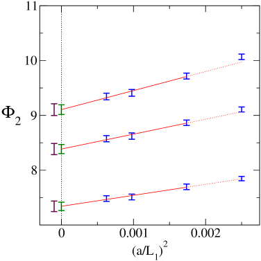
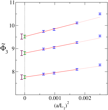
Figure 1: Continuum extrapolation of $\Phi_{2}(L_{1},M_{{\rm b}})$, for $z=10.4\,,\;12.1\,,\;13.3$ from bottom to top. The errors in the relation between bare quark mass $\widetilde{m}_{\rm q}$ and the RGI mass $M$ are translated into errors in $\Phi_{2}$. The $g_{0}$–independent part of that error is included after [?] the continuum extrapolation (left side error bar). On the right, the equivalent in the alternative strategy is shown for $\theta_{0}=1/2$ (see App. C).

We have performed a numerical computation in the quenched approximation, using the ${\rm O}(a)$ improved Wilson action [?,?,?]. The box size $L_{2}$ is chosen as $L_{2}=1.436r_{0}$, where $r_{0}$, defined in terms of the static quark potential [?], has a phenomenological value of $r_{0}\approx 0.5\,{\rm fm}$. From [?] we know the Schrödinger functional coupling $\bar{g}^{2}(L_{1})=\bar{g}^{2}(L_{2}/2)\approx 3.48$. Given the knowledge of $r_{0}/a$ as a function of $g_{0}$ of Ref. [?] and that of the renormalized coupling [?], it is then convenient to fix $g_{0}$ in different ways for the different steps of the calculation. The differences are of course only $a$-effects which disappear in the continuum extrapolations. We give more details below. We will take the uncertainties in the relations $\bar{g}^{2}(L_{1})\approx 3.48$ and $\bar{g}^{2}(L_{1}/4)\approx 1.8811$ (which we need later) into account in the very end.

In order to complete our definitions, we further choose $\theta_{0}=0$ and $\theta_{1},\theta_{2}\in\{0,1/2,1\}$. The different values of $\theta_{1},\theta_{2}$ offer the possibility to check whether our final results are independent of these arbitrary parameters as they should be up to small $1/m_{\mathrm{b}}^{2}$ terms. Simulation parameters as well as raw results are listed in tables in App. A and B.

5.1 QCD observables

For this part of the computation, we determined the bare parameters as in [?]: $g_{0}$ is fixed by requiring $\bar{g}^{2}(L_{1}/4)=1.8811$ for given resolutions $a/L$. The PCAC mass of the light quark, defined exactly as in that reference, is set to zero. Our heavy quark masses are chosen such that $z=M_{{\rm b}}\,L_{1}\approx 10-13$ . The bare parameters are listed in Table 3.

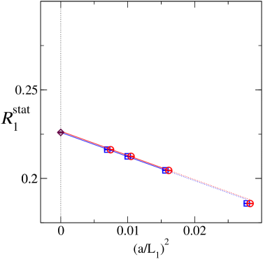
Figure 2: Continuum extrapolation of $\Phi_{1}(L_{1},M_{{\rm b}})$, separately for $R_{1}(L_{1},1/2,1)$ in QCD (left) and for $R^{\rm stat}_{1}(L_{1},1/2,1)$ in the static approximation (right). Circles denote results with action HYP1 and squares, displaced slightly for visibility, are from action HYP2. The corresponding continuum extrapolation lines are slightly displaced as well.

We focus our attention directly on the continuum extrapolations. As an example we show $\Phi_{1}(M_{{\rm b}},L_{1})$ and $\Phi_{2}(M_{{\rm b}},L_{1})$ in Fig. 2 and Fig. 1. Note that for the static subtraction $R^{\rm stat}_{1}(L_{1},1/2,1)$, displayed on the right of Fig. 2, our lattice spacings are roughly a factor three larger, since in the effective theory we only have to respect $a/L_{1}\ll 1$, not $aM_{{\rm b}}\ll 1$ (for details see App. A). Data have been obtained for two static actions, ${\rm HYP1}$ and HYP2[?]. In fitting them to the expected $a$-dependence, their continuum limit value is constrained to be independent of the action, but the $a^{2}$ slopes are of course different. The data for the different actions are highly correlated. As in all such cases, the errors of the continuum limit are computed from jacknife samples.

For values of $\theta_{i}$ which differ from the choice made in the figures, the $a$-dependence is very similar. In all these cases we find that extrapolations linear in $a^{2}$ using all four available lattice spacings are compatible with the ones where the data point at largest lattice spacing is ignored. We take the extrapolations with three points as our results for further analysis, since they have the more conservative error bars. The continuum limits are listed together with the raw numbers in Tables 6 and 4. From a fit of the continuum $\Phi_{2}(z)$ to a linear function, we then extract the slope

$$S={{\rm d}\over{\rm d}z}\Phi_{2}=0.61(5)\,$$ (5.73)

and we are done with the matching. The rest of the numerical computations is carried out in the effective theory.

5.2 HQET step scaling functions

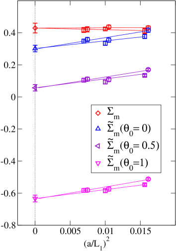
Figure 3: Continuum extrapolation of $\Sigma_{\rm m}$ and $\widetilde{\Sigma}_{\rm m}$.

Next we discuss the connection of $\Phi_{i}(L_{1},M_{{\rm b}})$ to $\Phi_{i}(L_{2},M_{{\rm b}})$, $L_{2}=2L_{1}$. It is given by the step scaling functions of Sect. 3.2. The bare parameters used in their computation are described in App. A, and the values at finite resolution $a/L_{1}$ are given in Tables 8-10 .

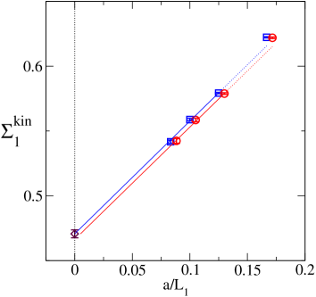
Figure 4: Continuum extrapolation of $\Sigma^{\mathrm{kin}}_{1}$ for $\theta_{1}=1/2,\theta_{2}=1$.

At lowest order in $1/m_{\mathrm{b}}$, only $\sigma_{\rm m}$ contributes. In its continuum extrapolation (Fig. 3, Table 8) we allow for a slope in $a^{2}$, although the data are compatible with a vanishing slope. Note that the absolute error of $\sigma_{\rm m}$ is negligible in comparison to twice the one of $\Phi_{2}$ (see Fig. 1) to which it is added in eq. (4.64). In fact the uncertainty in $\sigma_{\rm m}$ corresponds to an error of only $5\,{\rm MeV}$ in the b-quark mass, illustrating the possible precision in the static effective theory with these actions [?,?].

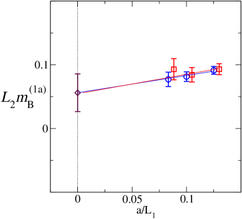
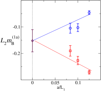
Figure 5: Lattice spacing dependence of $L_{2}m_{\rm B}^{(1a)}$ for $M_{\rm b}=M_{\rm b}^{(0)}$. On the left we show $m_{\rm B}^{(1a)}$ as introduced in Sect. 4, with $\theta_{1}=1/2,\;\theta_{2}=1$. We insert $\Phi_{1}$ in the continuum limit, such that the lattice spacing dependence is just due to $\Sigma^{\mathrm{kin}}_{2}$. On the right the corresponding quantity is shown for the alternative strategy of App. C, again with continuum values for $\widetilde{\Phi}_{i}$. There we set $\theta_{0}=1/2\;,\theta_{1}=1/2\;,\theta_{2}=1$.

A relevant question is how the precision deteriorates when one includes the first order corrections in $1/m_{\mathrm{b}}$. Then two more step scaling functions contribute. In Fig. 4, we illustrate how the continuum limit of $\sigma^{\mathrm{kin}}_{1}$ is obtained. Here we have to allow for a linear dependence on the lattice spacing, since the theory is not ${\rm O}(a)$ improved at the level of the $1/m_{\mathrm{b}}$ contributions [?]. Taking the more conservative fit with only three points, we arrive at the continuum limit listed in Table 9 for all combinations $\theta_{1},\theta_{2}$. In eq. (4.67), $\sigma^{\mathrm{kin}}_{1}$ is multiplied by small numbers (of order $1/m_{\mathrm{b}}$). This means that its error will be negligible in the overall error budget.

Instead of $\sigma^{\mathrm{kin}}_{2}$ we show directly the continuum extrapolation of $m_{\rm B}^{(1a)}$, eq. (4.66). As for $\Sigma_{\rm m}$, the data shows no significant $a$–dependence. Nevertheless, in order to have a realistic error estimate, we allow for a linear slope in $a$ (Fig. 5). In Table 10 we list the raw numbers for $\Sigma^{\mathrm{kin}}_{2}$ as well as the extracted continuum limit for further analysis.

5.3 Large volume matrix elements and $M_{{\rm b}}$

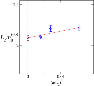
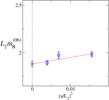
Figure 6: Lattice spacing dependence of $L_{2}m_{\rm B}^{(0b)}$, details as in Fig. 5.

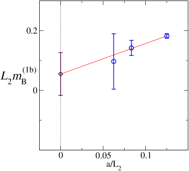
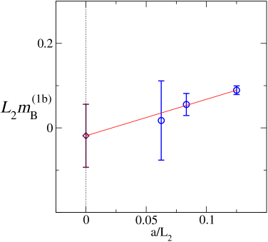
Figure 7: Lattice spacing dependence of $L_{2}m_{\rm B}^{(1b)}$, details as in Fig. 5.

The last missing pieces in eq. (2.30) are the large volume static energy $E_{\rm stat}$, eq. (2.24), and the matrix element of the kinetic operator $E_{\rm kin}$, eq. (2.28). Here, in contrast to the rest of our numerical evaluations, the light quark mass is set to the mass of the strange quark in order to avoid a chiral extrapolation. The spin averaged mass of the $B_{\mathrm{s}}$ system is then to be inserted into eq. (2.29).

Although $E_{\rm stat}$ and $E_{\rm kin}$ can be computed with periodic boundary conditions we here follow [?] and evaluate also these quantities with Schrödinger functional boundary conditions in a large volume of about $T\times(1.5{\rm fm})^{3}$, with $1.5{\rm fm}\leq T\leq 3{\rm fm}$ (also a check for finite size effects is carried out). The extraction is fairly standard, but still care has to be taken to make sure that the ground state contribution is obtained. This is a particularly relevant issue for B-physics, because the gap to the first excited state is rather small. We relegate details to App. B and discuss immediately the universal combinations $L_{2}m_{\rm B}^{(0b)}$, $L_{2}m_{\rm B}^{(1b)}$ which enter in eq. (2.30). The static contribution, shown in Fig. 6, is known with very good precision . In contrast, the $1/m_{\mathrm{b}}$ correction $L_{2}m_{\rm B}^{(1b)}$ does have a noticeable total uncertainty (Fig. 7, Table 1). Still, this error is only about 50% of the one on $2\Phi_{2}$. Note also that this error is almost entirely due to $E_{\rm kin}$ which may possibly be computed more precisely by other techniques [?].

We now have all pieces necessary to solve the equations for $M_{{\rm b}}$. The static one, eq. (4.70), is illustrated in Fig. 8. The horizontal error band is given by subtracting the static pieces $\sigma_{\rm m}+L_{2}m_{\rm B}^{(0b)}$ from the experimental number

$$m_{\rm B}^{\mathrm{av}}=5.405\,{\rm GeV}\,.$$ (5.74)

The figure demonstrates again that the main source of error is contained in the QCD computation of $\Phi_{2}$. Finally, by interpolating $\Phi_{i}(L_{1},M_{{\rm b}})$ to $M_{{\rm b}}=M_{{\rm b}}^{(0)}$ we obtain ($\theta_{1}=1/2,\theta_{2}=1$)

$$r_{0}\,M_{{\rm b}}^{(0)} = 17.25(20)\,,\;M_{{\rm b}}^{(0)}=6.806(79)\,{\rm GeV}\quad\mbox{for}\;r_{0}=0.5\,{\rm fm}$$ (5.75)

$$r_{0}\,M_{{\rm b}}^{(1)} = -0.12(9)\,,\;M_{{\rm b}}^{(1)}=-0.049(39)\,{\rm GeV}\quad\mbox{for}\;r_{0}=0.5\,{\rm fm}\,$$ (5.76)

$$r_{0}\,M_{{\rm b}} = 17.12(22)\,,\;M_{{\rm b}}=6.758(86)\,{\rm GeV}\quad\mbox{for}\;r_{0}=0.5\,{\rm fm}\,.$$ (5.77)

Here the small difference $\bar{g}^{2}(L_{1}/4)-1.8811$ as well as the statistical uncertainties in $\bar{g}^{2}(L_{1})$ and $L_{1}/r_{0}$ have been taken into account, as explained in App. D. Moreover, one can see in Table 1 that the $\theta_{i}$ dependence of the $1/m_{\mathrm{b}}$ contribution is absorbed.

$\theta_{1}$	$\theta_{2}$		$r_{0}M_{\rm b}^{(1a)}$	$r_{0}M_{\rm b}^{(1b)}$
0	1/2		-0.06(3)	-0.06(8)
1/2	1		-0.06(3)	-0.06(8)
1	0		-0.06(3)	-0.06(8)

Table 1: RGI results of $1/m_{\mathrm{b}}$ correction of the b-quark mass, in units of $r_{0}$.

With $\Lambda_{\rm\overline{MS\kern-0.35002pt}\kern 0.35002pt}r_{0}=0.602(48)$ [?,?], the 4-loop $\beta$ function and the mass anomalous dimension [?,?,?,?], we translate $M_{{\rm b}}=M_{{\rm b}}^{(0)}+M_{{\rm b}}^{(1)}$ to the mass in the ${\rm\overline{MS\kern-0.50003pt}\kern 0.50003pt}$ scheme at its own scale,

$$\kern 1.0pt\overline{\kern-1.0ptm\kern-1.0pt}\kern 1.0pt_{\rm b}(\kern 1.0pt\overline{\kern-1.0ptm\kern-1.0pt}\kern 1.0pt_{\rm b})=4.347(48){\rm GeV}\,;$$ (5.78)

the associated perturbative uncertainty can safely be neglected. For completeness we note that in the ${\rm\overline{MS\kern-0.50003pt}\kern 0.50003pt}$ scheme the $1/m_{\mathrm{b}}$ term amounts to $-27(22){\rm MeV}$.

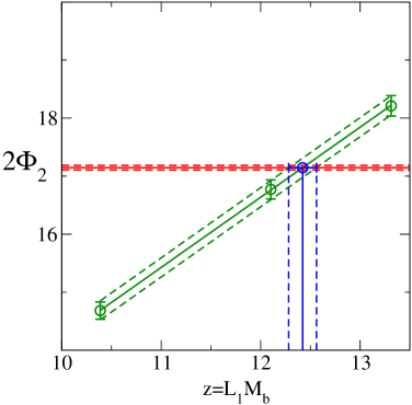
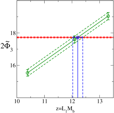
Figure 8: Graphical solution of eq. (4.70). On the left hand side, data points are $2\Phi_{2}$ and the horizontal error band is $L_{2}{m_{\rm B}^{\mathrm{av}}}-\sigma_{\rm m}-L_{2}[E^{\mathrm{stat}}-\Gamma^{\rm stat}_{1}(L_{2},\theta_{0})]$. On the right hand side, the analogous terms are shown for the alternative strategy ($\theta_{0}=1/2$, see Sect. 5.4).

5.4 Comparison to results from an alternative strategy

As mentioned earlier, at first sight it appears more natural to base the computation of $M_{{\rm b}}$ on the logarithmic derivative of the spin average of $f_{\rm A}$ and $k_{\rm V}$ as the prime finite volume quantity. We have not chosen this option as our standard strategy since then three observables are needed for matching. However, it is useful to consider also that alternative strategy in order to perform an explicit check that $1/m_{\mathrm{b}}^{2}$ terms are as small as expected. The results can be appreciated without detailed definitions of the observables and step scaling functions, the interested reader can find them in App. C. Here we note that within this alternative strategy we actually have nine different sets of $\{\widetilde{\Phi}_{1},\widetilde{\Phi}_{2},\widetilde{\Phi}_{3}\}$. Only one observable, $\widetilde{\Phi}_{1}=\Phi_{1}$, is in common to the two strategies. For our graphs we have selected (arbitrarily) one choice of parameters.

$\theta_{1}$	$\theta_{2}$	$r_{0}\,(M_{\rm b}^{(0)}+M_{\rm b}^{(1a)}+M_{\rm b}^{(1b)})$
			Main strategy		Alternative strategy
					$\theta_{0}=0$	$\theta_{0}=1/2$	$\theta_{0}=1$
0	1/2		17.12(22)		17.25(28)	17.23(28)	17.17(32)
1/2	1		17.12(22)		17.23(27)	17.21(27)	17.14(30)
1	0		17.12(22)		17.24(27)	17.22(28)	17.15(30)

Table 2: RGI results of $M_{\rm b}$ inlcuding the $1/m_{\mathrm{b}}$ correction, and comparison of the two strategies.

First, let us summarize what kind of differences one expects in such a comparison apart from $a$-effects. In the order of magnitude counting, we take $L_{1}^{-1}\sim\Lambda\sim 0.5\,{\rm GeV}$ and of course $L_{2}=2L_{1}$. The matching observables $\Gamma_{1},\Gamma^{\rm av}$ are constructed to be equal to the quark mass at the leading order in the HQET expansion. They start to differ at the next to leading order, which means by terms of order $\Lambda$. Also their dependence on $\theta_{i}$ is of that magnitude. Since $\Phi_{2}(L_{1},M_{{\rm b}})$ and $\tilde{\Phi}_{3}(L_{1},M_{{\rm b}})$ have been made dimensionless by multiplication with $L_{1}$ and $L_{1}$ happens to be around $\Lambda^{-1}$, the differences of $\Phi_{2}(L_{1},M_{{\rm b}})$ and $\tilde{\Phi}_{3}(L_{1},M_{{\rm b}})$ are order one. The step scaling functions $\sigma_{\rm m},\widetilde{\sigma}_{\rm m}$ as well as $L_{2}m_{\rm B}^{(0b)}$ are added to $\Phi_{2}$ (or $\tilde{\Phi}_{3}$) to obtain $L_{2}m_{\rm B}$ in static approximation. Thus they depend on the details at the same level, apart from a trivial $L_{2}/L_{1}=2$ factor. Of course, in the total static estimate $r_{0}M_{{\rm b}}^{(0)}$ this dependence is reduced to $r_{0}M_{{\rm b}}\times(\Lambda/m_{{\rm b}})^{2}\sim 1/5$. In the same way, the $1/m_{\mathrm{b}}$ corrections $L_{2}m_{\rm B}^{(1a)},L_{2}m_{\rm B}^{(1b)}$ themselves have a dependence on the matching conditions which is $L_{2}\times\Lambda^{2}/m_{{\rm b}}\sim 1/5$ but the final result $r_{0}M_{{\rm b}}$ including these terms is accurate and unique up to $r_{0}\times(\Lambda^{3}/m_{{\rm b}})^{2}\sim 1/50$ corrections.

We leave it to the reader to check in Fig. 1 to 7 that these expectations are fully satisfied by our results . In fact it appears that our estimate for the expansion parameter, $\Lambda/m_{{\rm b}}\sim 1/10$ is quite realistic. Of course, to find this out requires an explicit computation of the correction terms as presented here. In some cases, such as $m_{\rm B}^{(1b)}$, our precision is not good enough to resolve a dependence on the matching conditions.

In the b-quark mass in the static approximation, $r_{0}M_{{\rm b}}^{(0)}$ (eq. (5.75) and Table 12), the maximum difference is $0.5(2)$, which is of the predicted order of magnitude. Finally, when we add all contributions together, the results from the alternative strategy, Table 2, are fully in agreement with eq. (5.77). As expected $1/m_{\mathrm{b}}^{2}$ terms are not visible with our precision. They can safely be neglected.

6 Conclusions

The main conclusion of this work is that fully non-perturbative computations in lattice HQET, as they have been suggested in [?], are possible in practice. In particular, the uncertainties in the $1/m_{\mathrm{b}}$ corrections are smaller than those in the static approximation, despite the fact that we numerically cancel large $a^{-2}$ divergences in the $1/m_{\mathrm{b}}$ terms. The final error in the mass of the b-quark is dominated by the uncertainty in the renormalization in QCD. Errors due to simulations in the effective theory can almost be neglected in comparison.

A very nice result is the independence of the final numbers for $M_{{\rm b}}$ of the matching condition: Table 2 shows that within our reasonably small uncertainties, we get the same results for the quark mass for altogether twelve different matching conditions. This is expected up to very small terms of order $r_{0}M_{{\rm b}}\times(\Lambda/m_{{\rm b}})^{3}\sim 0.02$, which should be compared to our result $r_{0}M_{{\rm b}}=17.12(22)-17.25(28)$. Here the quoted range is due to the different matching conditions. In the order of magnitude estimates we have made a guess for the typical scale of $\Lambda\sim 0.5\,{\rm GeV}$. In the static approximation, some of the matching conditions yield slightly differing results for the quark mass in agreement with the expectation for such variations of $r_{0}M_{{\rm b}}\times(\Lambda/m_{{\rm b}})^{2}\sim 0.2$.

Both this explicit test of the magnitude of the different orders in the expansion and the naive order of magnitude estimate say that $1/m_{\mathrm{b}}^{2}$ corrections are completely negligible.

Still, in aspects of the computation, considerable improvement can be envisaged. For example, return to the $1/m_{\mathrm{b}}$ contribution to the B-meson mass Fig. 7. The statistical errors grow rapidly as one decreases the lattice spacing. The by far dominating uncertainty in the shown combination is the one of the large volume matrix $E_{\rm kin}$. It appears worth while to look for improvements, maybe along the line of [?]. Due to these errors, and of course the missing ${\rm O}(a)$-improvement of the theory at order $1/m_{\mathrm{b}}$ [?], the continuum extrapolation is not easy. Fortunately it is still precise enough for the present case. It will be very interesting to see cases where the $1/m_{\mathrm{b}}$ corrections are larger, as it is expected, for example, for $F_{\rm B}$.

Let us now turn to the computed value of $\kern 1.0pt\overline{\kern-1.0ptm\kern-1.0pt}\kern 1.0pt_{\rm b}$, eq. (5.78). Starting from a precisely specified input, namely $r_{0}$, $m_{\rm K}$ and $(m_{\rm B_{\rm s}}+3m_{\rm B_{\mathrm{s}}^{*}})/4$, the value of $M_{{\rm b}}$ is unambiguous in the quenched approximation, because these inputs fix the bare coupling, strange and beauty quark masses. We have used the experimental meson masses and $r_{0}=0.5\,{\rm fm}$. Our numbers for $M_{{\rm b}}$ or $\kern 1.0pt\overline{\kern-1.0ptm\kern-1.0pt}\kern 1.0pt_{\rm b}$ may then be used as a benchmark result for other methods. Indeed, a comparison shows agreement with [?] and the recent extension of that work [?] $\kern 1.0pt\overline{\kern-1.0ptm\kern-1.0pt}\kern 1.0pt_{\rm b}=4.42(7)\,{\rm GeV}$.

Earlier, the review [?] quoted $\kern 1.0pt\overline{\kern-1.0ptm\kern-1.0pt}\kern 1.0pt_{\rm b}=4.30(5)(5)\,{\rm GeV}$ and $\kern 1.0pt\overline{\kern-1.0ptm\kern-1.0pt}\kern 1.0pt_{\rm b}=4.34(3)(6)\,{\rm GeV}$, based on static computations [?] and an extrapolation of NRQCD results to the static limit [?] respectively. A perturbative subtraction [?,?,?] of the linear divergence $\delta m$ was carried out in these static estimates and, of course, a continuum extrapolation could not be done.

However, if other inputs are used, the result may change because $r_{0}$ is only approximately known and because the quenched approximation is not real QCD. A rough idea on the possible changes can be obtained by varying $r_{0}$ by $\pm 0.05\,{\rm fm}$. This changes $\kern 1.0pt\overline{\kern-1.0ptm\kern-1.0pt}\kern 1.0pt_{\rm b}(\kern 1.0pt\overline{\kern-1.0ptm\kern-1.0pt}\kern 1.0pt_{\rm b})$ by roughly $\,\pm 80\,{\rm MeV}$.

These remarks just serve to stress the obvious necessity of performing computations with $N_{\rm f}>0$. The ALPHA-collaboration is presently starting with $N_{\rm f}=2$, where the renormalization of the quark mass in QCD is known [?]. The necessary HQET computations are not expected to be a big numerical challenge, apart from the large volume B-meson matrix elements: simulations of the Schrödinger functional for $L\leq 1\,{\rm fm}$ are not very demanding with nowadays computing capabilities [?]. Altogether the extension of the present work to full QCD is feasible and should be carried out, since presently no better method is known to compute the b-quark mass from lattice QCD.

Acknowledgements. We thank Stephan Dürr for collaboration in the early stages of this work [?]. We thank NIC for allocating computer time on the APEmille computers at DESY Zeuthen to this project and the APE group for its help. This work is supported by the Deutsche Forschungsgemeinschaft in the SFB/TR 09.

Appendix A Finite volume simulations

$L\over a$	$\beta$	$\kappa_{\rm l}$	$\bar{g}^{2}({L\over 4})$	$Z_{\rm P}(g_{0},{L\over 2})$	$b_{\rm m}$	$Z$	$\kappa_{\rm h}$
$20$	$7.2611$	$0.134145$	$1.8811(19)$	$0.6826(3)$	$-0.621$	$1.0955$	$0.124195$
							$0.122119$
							$0.120483$
$24$	$7.4082$	$0.133961$	$1.8811(22)$	$0.6764(6)$	$-0.622$	$1.0941$	$0.126055$
							$0.124528$
							$0.123383$
$32$	$7.6547$	$0.133632$	$1.8811(28)$	$0.6713(8)$	$-0.622$	$1.0916$	$0.127991$
							$0.126967$
							$0.126222$
$40$	$7.8439$	$0.133373$	$1.8811(22)$	$0.6679(8)$	$-0.623$	$1.0900$	$0.128989$
							$0.128214$
							$0.127656$

Table 3: Bare parameters used in the computation of the QCD observables for $L=\tilde{L}_{1}$.

For the matching in a finite volume, we performed one set of simulations of (quenched) QCD and one of HQET. In the case of the relativistic theory, we used $L=\tilde{L}_{1}$, defined by $\bar{g}^{2}(\tilde{L}_{1}/4)=1.8811$ . The parameters of these simulations have been taken from [?] (see Table 3). The difference is that here $L=\tilde{L}_{1}=2\,\tilde{L}_{0}$ (and $T=L/2$ and $T=L/2\pm a$ in addition to $T=L$) compared to $L=\tilde{L}_{0}$ in [?].

The parameters for the resolution $\tilde{L}_{1}/a=20$ cannot be found in the mentioned reference. For that point, the gauge coupling $\beta$ has been chosen such that $\bar{g}^{2}(\tilde{L}_{1}/4)=1.8811$ for $\tilde{L}_{1}/4a=5$, see [?]. The renormalization constant $Z_{\rm P}$ and $\kappa_{\rm l}=\kappa_{\rm c}$ have been computed here, while $b_{\rm m}$ and $Z$ have been extrapolated from the values in Table 2 of [?]. These factors are put into the relationship between the bare mass $m_{\rm q,h}$ and the RGI mass [?,?],

$$M=h\,Z_{\rm m}\,m_{\rm q,h}\left(1+b_{\rm m}am_{\rm q,h}\right)\,,$$ (A.79)

where

$$Z_{\rm m}={{Z\;Z_{\rm A}}\over{Z_{\rm P}}}\;,\quad{\rm and}\quad am_{\rm q,h}={{1}\over{2}}\left({{1}\over{\kappa_{\rm h}}}-{{1}\over{\kappa_{\rm c}}}\right)\;.$$ (A.80)

The renormalization constant $Z_{\rm A}(g_{0}^{2})$ is known non-perturbatively from [?], while

$$h={{M}\over{\overline{m}(\mu_{0})}}=1.544(14)\;,\;\;\mu_{0}=2/\tilde{L}_{1}\;,$$ (A.81)

relates the running quark mass in the Schrödinger functional scheme [?] at the scale $\mu_{0}$, to the renormalization group invariant quark mass $M$ .

For all values of $\tilde{L}_{1}/a$ three hopping parameters $\kappa_{\rm h}$ have then been fixed in order to achieve

$$z=\tilde{L}_{1}\,M\;=\;10.4,\;12.1,\;13.3\,.$$ (A.82)

$L/a$	$z$	$R_{1}$			$\Phi_{2}$
		$\theta_{1}=0$	$\theta_{1}=1/2$	$\theta_{1}=1$	$\theta_{0}=0$
		$\theta_{2}=1/2$	$\theta_{2}=1$	$\theta_{2}=0$
$20$	$10.4$	$0.09795(13)$	$0.27426(30)$	$-0.37221(42)$	$7.847(40)$
$20$	$12.1$	$0.09512(12)$	$0.26588(30)$	$-0.36100(43)$	$9.108(46)$
$20$	$13.3$	$0.09336(12)$	$0.26068(30)$	$-0.35404(43)$	$10.068(50)$
$24$	$10.4$	$0.09958(18)$	$0.27904(37)$	$-0.37862(52)$	$7.697(44)$
$24$	$12.1$	$0.09689(17)$	$0.27110(37)$	$-0.36799(52)$	$8.866(50)$
$24$	$13.3$	$0.09528(17)$	$0.26632(36)$	$-0.36159(50)$	$9.716(54)$
$32$	$10.4$	$0.10157(30)$	$0.28481(71)$	$-0.38638(93)$	$7.512(53)$
$32$	$12.1$	$0.09897(30)$	$0.27717(71)$	$-0.37614(92)$	$8.623(58)$
$32$	$13.3$	$0.09744(30)$	$0.27265(71)$	$-0.37008(92)$	$9.411(62)$
$40$	$10.4$	$0.10283(30)$	$0.28806(52)$	$-0.39089(76)$	$7.484(51)$
$40$	$12.1$	$0.10027(30)$	$0.28052(52)$	$-0.38079(75)$	$8.575(56)$
$40$	$13.3$	$0.09876(29)$	$0.27608(52)$	$-0.37484(74)$	$9.344(60)$
$CL$	$10.4$	$0.10450(44)$	$0.29297(89)$	$-0.39748(125)$	$7.341(96)$
$CL$	$12.1$	$0.10202(44)$	$0.28567(90)$	$-0.38769(124)$	$8.386(102)$
$CL$	$13.3$	$0.10058(44)$	$0.28143(91)$	$-0.38202(124)$	$9.106(107)$

Table 4: Simulation results of the finite volume ($L=\tilde{L}_{1}$) relativistic observables needed in our main strategy. The continuum limits, obtained by linear extrapolation in $(a/L)^{2}$ of the results for $L/a\geq 24$, are indicated by CL.

$L/a$	$z$	$R_{\rm av}$			$\tilde{\Phi}_{3}$
		$\theta_{1}=0$	$\theta_{1}=1/2$	$\theta_{1}=1$	$\theta_{1}=0$	$\theta_{1}=1/2$	$\theta_{1}=1$
		$\theta_{2}=1/2$	$\theta_{2}=1$	$\theta_{2}=0$
$20$	$10.4$	$0.1699(9)$	$0.4299(12)$	$-0.5998(20)$	$8.059(37)$	$8.293(37)$	$8.993(37)$
$20$	$12.1$	$0.1668(9)$	$0.4198(11)$	$-0.5867(20)$	$9.315(37)$	$9.545(37)$	$10.234(37)$
$20$	$13.3$	$0.1649(9)$	$0.4137(11)$	$-0.5787(19)$	$10.271(37)$	$10.500(37)$	$11.180(37)$
$24$	$10.4$	$0.1739(23)$	$0.4391(31)$	$-0.6130(54)$	$7.864(39)$	$8.102(38)$	$8.822(39)$
$24$	$12.1$	$0.1710(23)$	$0.4295(30)$	$-0.6005(52)$	$9.027(39)$	$9.263(38)$	$9.971(39)$
$24$	$13.3$	$0.1693(22)$	$0.4239(29)$	$-0.5931(51)$	$9.874(39)$	$10.109(38)$	$10.809(38)$
$32$	$10.4$	$0.1760(41)$	$0.4494(48)$	$-0.6254(90)$	$7.713(43)$	$7.941(41)$	$8.661(42)$
$32$	$12.1$	$0.1733(40)$	$0.4403(46)$	$-0.6135(87)$	$8.818(42)$	$9.045(41)$	$9.753(42)$
$32$	$13.3$	$0.1717(40)$	$0.4349(45)$	$-0.6066(85)$	$9.603(42)$	$9.828(41)$	$10.531(42)$
$40$	$10.4$	$0.1790(70)$	$0.4493(72)$	$-0.6283(142)$	$7.656(45)$	$7.894(42)$	$8.624(44)$
$40$	$12.1$	$0.1763(68)$	$0.4403(70)$	$-0.6166(138)$	$8.743(45)$	$8.979(42)$	$9.698(44)$
$40$	$13.3$	$0.1747(67)$	$0.4352(68)$	$-0.6099(136)$	$9.509(45)$	$9.744(42)$	$10.456(44)$
$CL$	$10.4$	$0.1801(75)$	$0.4587(84)$	$-0.6392(159)$	$7.533(89)$	$7.765(86)$	$8.496(88)$
$CL$	$12.1$	$0.1776(73)$	$0.4502(81)$	$-0.6280(154)$	$8.573(91)$	$8.805(88)$	$9.524(89)$
$CL$	$13.3$	$0.1761(72)$	$0.4452(79)$	$-0.6218(151)$	$9.289(93)$	$9.519(91)$	$10.234(92)$

Table 5: Same as Table 4 in the case of the alternative strategy.

We collect these parameters in Table 3, whereas the results for the quantities needed in the matching step are summarized in Tables 4 and 5. The errors there include systematics due to the uncertainties in the $Z$-factors, in particular, the error on the universal factor $h$ has been propagated only after performing the continuum limit extrapolations. Ensembles of roughly 2000 (for $\tilde{L}_{1}/a=20$) to few hundreds (for $\tilde{L}_{1}/a=40$) gauge configurations have been generated for this part of the computation. The lattice $\tilde{L}_{1}/a=20$ is not used in the extrapolations but rather to check for the smallness of higher order cutoff effects for $\tilde{L}_{1}/a\geq 24$.

Concerning the simulation of HQET, we have computed the various quantities in the two required volumes. The first one, where we match the effective theory with QCD, has a space extent $L_{1}$. The second one is such that $L_{2}=2L_{1}$. The value of the Schrödinger functional renormalized coupling is fixed at $\bar{g}^{2}(L_{1})=3.48$, and we have used the resolutions $L_{1}/a=6,8,10,12$. The corresponding values of $\beta$ as well as $\kappa=\kappa_{c}$ can be found in Table A.1 of [?]. All these quantities are computed with two different actions, HYP1 and HYP2. The continuum values are then obtained by constraining the fits to give the same values for these actions. We note that the results for HYP1 and HYP2 are statistically correlated.

$L/a$	$R_{1}^{\rm stat}$
	$\theta_{1}=0$			$\theta_{1}=1/2$			$\theta_{1}=1$
	$\theta_{2}=1/2$			$\theta_{2}=1$			$\theta_{2}=0$
	HYP1	HYP2		HYP1	HYP2		HYP1	HYP2
6	0.06936(5)	0.06939(4)		0.18583(7)	0.18591(7)		-0.25519(12)	-0.25530(11)
8	0.07572(6)	0.07574(6)		0.20452(11)	0.20457(11)		-0.28024(17)	-0.28031(17)
10	0.07821(5)	0.07822(5)		0.21246(8)	0.21249(8)		-0.29067(13)	-0.29071(13)
12	0.07934(8)	0.07935(8)		0.21622(13)	0.21625(13)		-0.29556(21)	-0.29559(20)
CL	0.08238(12)			0.22596(21)			-0.30835(32)

Table 6: Lattice results of $R_{1}^{\rm stat}$ for $L=L_{1}$. The continuum limits are obtained by a linear extrapolation in $(a/L)^{2}$ of the results for $L/a\geq 8$.

$L/a$	$R_{\rm av}^{\rm stat}$
	$\theta_{1}=0$			$\theta_{1}=1/2$			$\theta_{1}=1$
	$\theta_{2}=1/2$			$\theta_{2}=1$			$\theta_{2}=0$
	HYP1	HYP2		HYP1	HYP2		HYP1	HYP2
6	0.1502(3)	0.1543(3)		0.3562(3)	0.3688(3)		-0.5231(6)	-0.5231(6)
8	0.1544(4)	0.1575(4)		0.3672(4)	0.3765(4)		-0.5216(7)	-0.5340(8)
10	0.1571(5)	0.1595(5)		0.3724(6)	0.3710(6)		-0.5295(10)	-0.5391(10)
12	0.1561(8)	0.1579(8)		0.3729(8)	0.3786(9)		-0.5289(15)	-0.5365(16)
CL	0.1606(6)			0.3827(6)			-0.5432(11)

Table 7: Lattice results of $R_{\rm av}^{\rm stat}$. The details are the same as in Table 6.

For the computation of the step scaling functions one uses the same $\beta,\kappa$ and $L_{2}/a=2L_{1}/a$. All these computations are done with several thousand gauge configurations. Note that, even if $L_{1}$ is the same in QCD and in HQET, the typical lattice spacings are much larger in the effective theory. The results of $R_{1}^{\rm stat}$ and $R_{\rm av}$ can be found in Tables 6 and 7. The values of the step scaling functions are collected in Tables 8, 9 and 10.

$L/a$	$\Sigma_{\rm m}(3.48,a/L)$
	HYP1	HYP2
8	0.431(11)	0.411(11)
10	0.437(11)	0.424(10)
12	0.422(16)	0.418(16)
CL	0.430(25)

Table 8: Lattice results of the step scaling function $\Sigma_{\rm m}$. The bare parameters are described in the text. The continuum limit is obtained by a linear extrapolation in $(a/L)^{2}$ of the results for $L/a\geq 8$.

$L/a$	$\Sigma_{1}^{\mathrm{kin}}(3.48,a/L)$
	$\theta_{1}=0$			$\theta_{1}=1/2$			$\theta_{1}=1$
	$\theta_{2}=1/2$			$\theta_{2}=1$			$\theta_{2}=0$
	HYP1	HYP2		HYP1	HYP2		HYP1	HYP2
6	0.6241(17)	0.6245(11)		0.6219(60)	0.6223(5)		0.6225(8)	0.6228(6)
8	0.5790(20)	0.5797(13)		0.5789(65)	0.5793(5)		0.5789(10)	0.5794(7)
10	0.5587(47)	0.5586(22)		0.5585(14)	0.5588(9)		0.5586(22)	0.5590(14)
12	0.5364(66)	0.5342(39)		0.5424(19)	0.5417(12)		0.5409(30)	0.5398(18)
CL	0.457(10)			0.471(3)			0.467(5)

Table 9: Lattice results of the step scaling function $\Sigma_{1}^{\mathrm{kin}}$. The continuum limits are obtained by a linear extrapolation in $a/L$ of the results for $L/a\geq 8$.

$L/a$	$\Sigma_{2}^{\mathrm{kin}}(3.48,a/L)$
	$\theta_{1}=0$			$\theta_{1}=1/2$			$\theta_{1}=1$
	$\theta_{2}=1/2$			$\theta_{2}=1$			$\theta_{2}=0$
	HYP1	HYP2		HYP1	HYP2		HYP1	HYP2
8	4.81(44)	4.72(32)		1.58(15)	1.55(10)		-1.19(11)	-1.17(8)
10	4.34(58)	4.20(39)		1.43(19)	1.39(13)		-1.08(15)	-1.04(10)
12	4.79(86)	3.98(58)		1.58(28)	1.31(19)		-1.19(21)	-0.99(14)
CL	2.9(1.5)			0.96(50)			-0.71(38)

Table 10: Same as Table 9 for $\Sigma_{2}^{\mathrm{kin}}$.

Finally there are simulations in small volume to obtain the subtractions $\Gamma^{\rm stat}_{1}(L_{2})$ and $\Gamma^{\rm kin}_{1}(L_{2})$. These are done with $L_{2}=1.436\,r_{0}$ and $\beta$ determined from the knowledge of $r_{0}/a$ [?]. The parameters, including $\kappa=\kappa_{c}$, are listed in Table 6 of [?]. The values of $\beta$ do of course agree with the ones employed in the large volume, which we describe in the next appendix.

Appendix B Large volume simulations and extraction of matrix elements

The parameters for the simulations in large volume are collected in Table 11 together with the results for $E_{\rm stat}$ and $E_{\rm kin}$. The lattice extension $L/a$ and $\beta$ are such that $L=4L_{1}\approx 3/2\,{\rm fm}$ except for the second lattice where we have $L=6L_{1}\approx 2\,{\rm fm}$. This lattice is used only to check for the absence of finite size effects. We see from Table 11 that finite size effects are indeed very small, the difference between the results from the $L/a=16$ and the $L/a=24$ lattices at $\beta=6.0219$ is consistent with zero within at most one standard deviation ($aE_{\rm stat}$ from HYP1). The number of configurations generated ranges from $4300$ at $\beta=6.0219$ to $2200$ at $\beta=6.4956$ (for the larger volume at $\beta=6.0219$ we had $1300$ configurations). Since our phenomenological input is the mass of the (spin averaged) $B_{\rm s}$ meson, we set $\kappa$ to $\kappa_{\rm s}$ in order to reproduce the quenched value of the strange quark mass from Ref. [?], i.e.

$$M_{\rm s}r_{0}=0.35(1)\;,$$ (B.83)

with $M_{\rm s}$ the renormalization group invariant strange quark mass defined as in Appendix A after replacing $\kappa_{\rm h}$ by $\kappa_{\rm s}$.

$\beta$	$\kappa_{\rm s}$	$L^{3}\times T$	$aE_{\rm stat}$		$a^{2}E_{\rm kin}$
			HYP1	HYP2	HYP1	HYP2
$6.0219$	$0.133849$	$16^{3}\times 24\;[32]$	$0.4345(21)$	$0.4029(32)$	$0.750(4)$	$0.774(3)$
$6.0219$	$0.133849$	$24^{3}\times 32$	$0.4378(25)$	$0.4034(20)$	$0.746(7)$	$0.776(5)$
$6.2885$	$0.1349798$	$24^{3}\times 48$	$0.3295(21)$	$0.3034(29)$	$0.643(7)$	$0.676(5)$
$6.4956$	$0.1350299$	$32^{3}\times 64$	$0.2724(20)$	$0.2461(14)$	$0.599(10)$	$0.620(11)$

Table 11: Parameters of the large volume simulations. Where present, the numbers in brackets refer to a second dataset at the same $(\beta,\kappa)$ values.

The numbers for $E_{\rm stat}$ and $E_{\rm kin}$ have been obtained by applying two different fitting procedures to two independent datasets (where available). The quoted errors are such that both the results are covered and they therefore provide a reasonable estimate of the systematics associated with the fits. We now sketch these procedures.

Let us consider in QCD the effective “mass” $\Gamma(x_{0})$ obtained from the correlation function $F_{\rm av}(x_{0})$ in eq. (C.93) and its quantum-mechanical decomposition

$$\Gamma(x_{0})=-{{\partial_{0}+\partial^{*}_{0}}\over{2}}F_{\rm av}=E_{0}+Ae^{-\Delta x_{0}}+\dots$$ (B.84)

where $E_{0}$ is the energy of the ground state, $\Delta$ is the gap between the ground and the first excited states and the dots refer to contributions from higher states. The $1/m_{\rm b}$ expansion reads

$$\Gamma(x_{0}) = E_{\rm stat}+\omega_{\rm kin}E_{\rm kin}+(A^{\rm stat}+\omega_{\rm kin}A^{\rm kin})e^{-\Delta^{\rm stat}x_{0}}(1-\omega_{\rm kin}x_{0}\Delta^{\rm kin})+\dots$$ (B.85)

$$= \Gamma^{\rm stat}(x_{0})+\omega_{\rm kin}\Gamma^{\rm kin}(x_{0})+\dots$$

where $\Gamma^{\rm stat}$ and $\Gamma^{\rm kin}$ are defined in analogy to eqs. (3.55, 3.56) in terms of the correlators $f_{\rm A}^{\rm stat}(x_{0})$ and $f_{\rm A}^{\rm kin}(x_{0})$.

In the correlation function $f_{\delta{\rm A}}(x_{0})$ the same states contribute as in $f_{\rm A}(x_{0})$. Performing again first the quantum-mechanical decomposition and then the $1/m_{\rm b}$ expansion of these correlators, it is easy to see that the ratios

$$P_{\rm A}^{\rm stat}(x_{0})={{f_{\rm A}^{\rm stat}(x_{0})}\over{f_{\delta\rm A}^{\rm stat}(x_{0})}}\quad{\rm and}\quad P_{\rm A}^{\rm kin}(x_{0})=P_{\rm A}^{\rm stat}(x_{0})\left[{{f_{\rm A}^{\rm kin}(x_{0})}\over{f_{\rm A}^{\rm stat}(x_{0})}}-{{f_{\delta\rm A}^{\rm kin}(x_{0})}\over{f_{\delta\rm A}^{\rm stat}(x_{0})}}\right]$$ (B.86)

have the following form

$$P_{\rm A}^{\rm stat} = b_{1}+b_{2}e^{-\Delta^{\rm stat}x_{0}}\;,$$ (B.87)

$$P_{\rm A}^{\rm kin} = b_{3}+b_{4}e^{-\Delta^{\rm stat}x_{0}}-b_{2}\Delta^{\rm kin}x_{0}e^{-\Delta^{\rm stat}x_{0}}\;.$$ (B.88)

They can therefore be used to further constrain $\Delta^{\rm stat}$ and $\Delta^{\rm kin}$. We are thus lead to perform a combined fit

$$\Gamma^{\rm stat} = b_{5}+b_{6}e^{-\Delta^{\rm stat}x_{0}}\;,$$ (B.89)

$$\Gamma^{\rm kin} = b_{7}+b_{8}e^{-\Delta^{\rm stat}x_{0}}-b_{6}\Delta^{\rm kin}x_{0}e^{-\Delta^{\rm stat}x_{0}}\;,$$ (B.90)

together with eq. (B.87) and (B.88), with non-linear parameters $a_{1}=\Delta^{\rm stat}$ and $a_{2}=\Delta^{\rm kin}$ and the linear parameters $b_{i}$, which contain the desired $b_{5}=E_{\rm stat}$ and $b_{7}=E_{\rm kin}$.

Since the correction terms are nevertheless not so easy to compute at the smaller lattice spacings, we perform the above fit first at $\beta=6.0219$ and extract $a\Delta^{\rm stat}$ and $a^{2}\Delta^{\rm kin}$. We then use that these quantities scale roughly (i.e. $r_{0}\,\Delta^{\rm stat}\approx$constant and $r_{0}^{2}\,\Delta^{\rm kin}\approx$constant). To implement this, we input the scaled means as priors [?] in a second step where we add

$$\chi^{2}_{\rm prior}=\sum_{i=1,2}{{\left(a_{i}-a_{1}^{\rm prior}\right)^{2}}\over{(\delta a_{i}^{\rm prior})^{2}}}\;,$$ (B.91)

to the standard $\chi^{2}$. The uncertainty $\delta a_{i}^{\rm prior}$ is taken from the fit result at $\beta=6.0219$. However, in order to remain on the safe side, it is not scaled but kept constant at the smaller lattice spacing. Thus $\delta a_{2}^{\rm prior}/a_{2}^{\rm prior}\propto 1/a^{2}$ for example. The constraint due to the priors becomes weaker as we approach the continuum.

Here and in the following procedure the fit range is chosen to keep a minimum physical distance from the boundaries, namely $x_{0}\geq t_{\rm min}\approx 2r_{0}$. The stability of the results is checked by varying $t_{\rm min}$ to $t_{\rm min}-r_{0}/2$. As an example we show in figure 9 the results for $P_{\rm A}^{\rm stat},\,P_{\rm A}^{\rm kin},\,\Gamma^{\rm stat}$ and $\Gamma^{\rm kin}$ at $\beta=6.2885$. One observes that $P_{\rm A}^{\rm stat},\,\Gamma^{\rm stat}$ provide very good constraints of the parameters $\Delta^{\rm stat},\,b_{2},\,b_{6}$. The remaining ones are then effectively linear fit parameters. Nevertheless, the error band of $E_{\rm kin}$ (dashed line) resulting from the fit is not that small.

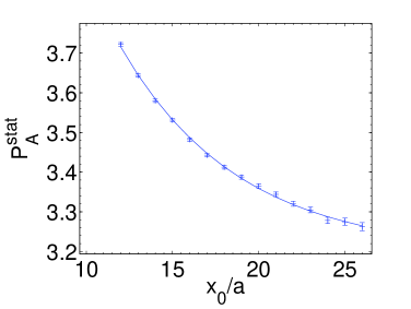
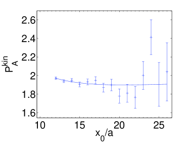
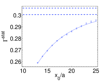
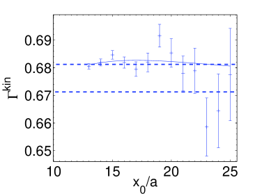
Figure 9: Results for $P_{\rm A}^{\rm stat}$, $P_{\rm A}^{\rm kin}$, $\Gamma^{\rm stat}$ and $\Gamma^{\rm kin}$ at $\beta=6.2885$ (HYP2) with the corresponding functions obtained by the fit.

An alternative strategy is used to get a second estimate of $E_{\rm stat}$ at the two coarser lattice spacings, where we have two independent datasets. Exploiting again the remark before eq. (B.86) we construct an effective mass $\Gamma_{\delta\rm A}$ from the correlator $f_{\delta\rm A}(x_{0})$ in the very same way as $\Gamma^{\rm stat}$ is obtained from $f_{\rm A}^{\rm stat}(x_{0})$. The idea is to combine the two effective masses in order to eliminate the contribution from the first excited state and then perform a fit to a constant (in the mentioned fit range). In practice we minimize the quantity

$$Q=\sum_{x_{0}=t_{\rm min}}^{t_{\rm max}}\left[\Gamma^{\rm stat}(x_{0})+\alpha\Gamma_{\delta{\rm A}}(x_{0})-B\right]^{2}\;,$$ (B.92)

with respect to $\alpha,\;B$. Finally the weighted average of $\left[\Gamma^{\rm stat}(x_{0})+\alpha\Gamma_{\delta{\rm A}}(x_{0})\right]/(1+\alpha)$ yields the estimate of $E^{\rm stat}$. The quality of the result is comparable to that obtained in the first approach.

Appendix C Alternative strategy

We briefly introduce an alternative strategy, based on the correlation functions $f_{\rm A},k_{\rm V}$ in addition to $f_{1},k_{1}$. With

$$F_{\mathrm{av}}(x_{0},\theta)={1\over 4}\log\left(-\left[f_{\rm A}\right]_{\mathrm{R}}(x_{0},\theta)\times\left[k_{\rm V}\right]_{\mathrm{R}}^{3}(x_{0},\theta)\right)$$ (C.93)

we introduce

$$R_{\mathrm{av}}(L,\theta_{1},\theta_{2}) = F_{\mathrm{av}}(x_{0},\theta_{1})-F_{\mathrm{av}}(x_{0},\theta_{2})\;\mbox{at}\;x_{0}=L/2\,,\;T=L$$ (C.94)

$$\Gamma^{\rm av}(L,\theta_{0}) = -{\partial_{0}+\partial_{0}^{*}\over 2}F_{\mathrm{av}}(x_{0},\theta_{0})\;\mbox{at}\;x_{0}=L/2\,,\;T=L\,.$$ (C.95)

Keeping $\Phi_{1}$, from the standard strategy, we define the set of observables

$$\widetilde{\Phi}_{1}(L,M_{{\rm b}}) = \Phi_{1}(L,M_{{\rm b}})\,,$$ (C.96)

$$\widetilde{\Phi}_{2}(L,M_{{\rm b}}) = R_{\mathrm{av}}(L,\theta_{1},\theta_{2})-R_{\mathrm{av}}^{\mathrm{stat}}(L,\theta_{1},\theta_{2})\,,$$ (C.97)

$$\widetilde{\Phi}_{3}(L,M_{{\rm b}}) = L\Gamma^{\rm av}(L,\theta_{0})\,,$$ (C.98)

with the $1/m_{\mathrm{b}}$ expansion

$$\widetilde{\Phi}_{2}(L,M_{{\rm b}}) = \omega_{\mathrm{kin}}R^{\rm kin}_{\rm A}(L,\theta_{1},\theta_{2})+c_{\rm av}^{\rm HQET}R_{\delta\rm A}(L,\theta_{1},\theta_{2})\,$$ (C.99)

$$\widetilde{\Phi}_{3}(L,M_{{\rm b}}) = L\,\big{[}m_{\rm bare}+\Gamma^{\rm stat}(L,\theta_{0})+\omega_{\mathrm{kin}}\Gamma^{\rm kin}(L,\theta_{0})+c_{\rm av}^{\rm HQET}\Gamma_{\delta A}(L,\theta_{0})\big{]}\,,$$ (C.100)

where due to the spin average the combination

$$c_{\rm av}^{\rm HQET}={1\over 4}[c_{\rm A}^{\rm HQET}+3c_{\rm V}^{\rm HQET}]$$ (C.101)

is present. The so far undefined terms $R_{\mathrm{av}}^{\mathrm{stat}},R^{\rm kin}_{\rm A},\Gamma^{\rm kin},R_{\delta\rm A},\Gamma_{\delta A}$ are straightforwardly obtained from our definitions.

The alternative observables change from $L$ to $2L$ via

$$\widetilde{\Phi}_{i}(2L,M_{{\rm b}}) = \sum_{j\leq i}\sigma_{ij}(u)\,\widetilde{\Phi}_{j}(L,M_{{\rm b}})\;+\;\delta_{i3}\;\widetilde{\sigma}_{\rm m}(u)\,,$$ (C.102)

$$\sigma_{ij}(u) = \lim_{a/L\to 0}\Sigma_{ij}(u,a/L)$$ (C.103)

with the step scaling functions (we drop arguments $\theta_{1},\theta_{2}$ and $u=\bar{g}^{2}(L)$ is understood)

$$\Sigma_{11}(u,a/L) = R^{\rm kin}_{1}(2L)/R^{\rm kin}_{1}(L)=\Sigma_{1}^{\mathrm{kin}}(u,a/L)$$ (C.104)

$$\Sigma_{21}(u,a/L) = {1\over R^{\rm kin}_{1}(L)}\{R^{\rm kin}_{\rm A}(2L)-R^{\rm kin}_{\rm A}(L)\,\Sigma_{22}(u,a/L)\}$$ (C.105)

$$\Sigma_{22}(u,a/L) = R_{\delta\rm A}(2L)/R_{\delta\rm A}(L)$$ (C.106)

$$\Sigma_{31}(u,a/L) = {2L\{\Gamma^{\rm kin}(2L)-\Gamma^{\rm kin}(L)\}\over R^{\rm kin}_{1}(L)}-\,\Sigma_{32}(u,a/L){R^{\rm kin}_{\rm A}(L)\over R^{\rm kin}_{1}(L)}$$ (C.107)

$$\Sigma_{32}(u,a/L) = 2L{\Gamma_{\delta A}(2L)-\Gamma_{\delta A}(L)\over R_{\delta\rm A}(L)}$$ (C.108)

$$\Sigma_{33}(u,a/L) = 2$$ (C.109)

$$\widetilde{\sigma}_{\rm m}(u) = \lim_{a/L\to 0}2L\,\big{[}\Gamma^{\rm stat}(2L)-\Gamma^{\rm stat}(L)\big{]}\,.$$ (C.110)

The final relation for the B-meson mass is eq. (2.30) with

$$L_{2}m_{\mathrm{B}}^{\mathrm{(0a)}}(M_{{\rm b}}) = \widetilde{\sigma}_{\rm m}(u_{1})+2\,\widetilde{\Phi}_{3}(L_{1},M_{{\rm b}})\,,$$ (C.111)

$$L_{2}m_{\mathrm{B}}^{\mathrm{(0b)}}(M_{{\rm b}}) = L_{2}[E^{\mathrm{stat}}-\Gamma^{\rm stat}(L_{2})]\,,$$ (C.112)

$$L_{2}m_{\rm B}^{(1a)}(M_{{\rm b}}) = \sigma_{31}(u_{1})\,\widetilde{\Phi}_{1}(L_{1},M_{{\rm b}})+\sigma_{32}(u_{1})\,\widetilde{\Phi}_{2}(L_{1},M_{{\rm b}})\,,$$ (C.113)

$$L_{2}m_{\rm B}^{(1b)}(M_{{\rm b}}) = L_{2}\left[{E^{\mathrm{kin}}-\Gamma^{\rm kin}(L_{2})\over R^{\rm kin}_{1}(L_{2})}+{\Gamma_{\delta A}(L_{2})\,R^{\rm kin}_{\rm A}(L_{2})\over R_{\delta\rm A}(L_{2})\,R^{\rm kin}_{1}(L_{2})}\right]\,\sigma^{\mathrm{kin}}_{1}(u_{1})\,\widetilde{\Phi}_{1}(L_{1},M_{{\rm b}})$$ (C.114)

$$-L_{2}{\Gamma_{\delta A}(L_{2})\over R_{\delta\rm A}(L_{2})}\left[\sigma_{21}(u_{1})\,\widetilde{\Phi}_{1}(L_{1},M_{{\rm b}})+\sigma_{22}(u_{1})\,\widetilde{\Phi}_{2}(L_{1},M_{{\rm b}})\right]\,.$$

Although the results have been already given in Table 2, the reader will find more details in Table 12.

$\theta_{0}$	$r_{0}M_{\rm b}^{(0)}$		$r_{0}M_{\rm b}^{(1a)}$				$r_{0}M_{\rm b}^{(1b)}$
			$\theta_{1}=0$	$\theta_{1}=1/2$	$\theta_{1}=1$		$\theta_{1}=0$	$\theta_{1}=1/2$	$\theta_{1}=1$
			$\theta_{2}=1/2$	$\theta_{2}=1$	$\theta_{2}=0$		$\theta_{2}=1/2$	$\theta_{2}=1$	$\theta_{2}=0$
0	17.05(25)		0.17(6)	0.17(6)	0.17(6)		0.02(9)	0.02(8)	0.02(9)
1/2	17.01(22)		0.20(7)	0.18(6)	0.19(7)		0.02(10)	0.02(9)	0.02(9)
1	16.78(28)		0.34(11)	0.30(7)	0.32(8)		0.06(12)	0.06(9)	0.06(10)

Table 12: RGI results of $M_{\rm b}$ in the static approximation and of the $1/m_{\mathrm{b}}$ correction for the alternative strategy.

Appendix D Propagating uncertainties in $L_{i}/r_{0}$ and $\bar{g}^{2}(L_{i})$

In our simulations we have fixed $\tilde{L}_{1}$ by $\bar{g}^{2}(\tilde{L}_{1}/4)=1.8811$, because the corresponding bare parameters $\beta,\kappa$ are available in the literature. We here give the estimate of the small effect caused by $\tilde{L}_{1}\neq L_{1}$ in the static approximation. From the polynomial interpolations of the step scaling function of the coupling, $\sigma(u)$ [?], we estimate the corresponding mismatch in couplings as

$$\tilde{u}-u=\bar{g}^{2}(\tilde{L}_{1})-\bar{g}^{2}(L_{1})=\sigma(\sigma(1.8811))-3.48=-0.17(5)\,.$$ (D.115)

Let us write

$${M_{{\rm b}}\over m_{\mathrm{B}}}=\rho(\tilde{u},z)\,[1+K(u)]\quad\mbox{at}\quad\tilde{u}=u$$ (D.116)

with

$$K(u)={\Gamma^{\rm stat}_{1}(L_{1})-E_{\rm stat}\over m_{\mathrm{B}}}\,,\quad\rho(u,z)={z\over\Phi_{2}(u,z)}\,.$$ (D.117)

The relation ${{\rm d}\over{\rm d}u}{M_{{\rm b}}\over m_{\mathrm{B}}}=0$ gives

$$-{1+K(u)\over\rho(u,z)}{{\rm d}\over{\rm d}u}\rho(u,z)=K^{\prime}(u)={1\over m_{\mathrm{B}}}{{\rm d}\over{\rm d}u}\Gamma^{\rm stat}_{1}\,.$$ (D.118)

Denoting by $\Delta M_{{\rm b}}$ the correction we have to add to $M_{{\rm b}}$ when it is computed with $\tilde{u}\neq u$ (as we did), we get from the above equations

$${1\over m_{\mathrm{B}}}\Delta M_{{\rm b}}=[\tilde{u}-u]\times\rho(u)K^{\prime}(u)\,,$$ (D.119)

where $K^{\prime}(u)$ is easily estimated by taking a numerical derivative of $\Gamma^{\rm stat}_{1}$. From the difference of $L/a=12$ and $L/a=10$ at fixed $g_{0}^{2}$ (with $\bar{g}^{2}|_{L/a=12}=3.48$) and with $\rho(u,z)\approx 1.44$ we arrive at the small shift

$$r_{0}\Delta M_{{\rm b}} = -0.055(17)\,.$$ (D.120)

A similar error is be taken into account due to the 2% uncertainty in the relation $L_{2}=1.436r_{0}$ [?]. In the same way it leads to a statistical error of

$$r_{0}\Delta M_{{\rm b}} = 0.016\,.$$ (D.121)

The two contributions eq. (D.120), eq. (D.121) are combined to

$$r_{0}\Delta M_{{\rm b}} = -0.055(23)\,,$$ (D.122)

which we have taken into account in Sect. 5.3. Because of the smallnes of these effects, they can be neglected in the $1/m_{\mathrm{b}}$-corrections.

In the case of our alternative strategy, the shift depdends on the value of $\theta_{0}$. We find

$$\theta_{0}=0 \qquad r_{0}\Delta M_{{\rm b}}=-0.042(20)\,,$$ (D.123)

$$\theta_{0}=1/2 \qquad r_{0}\Delta M_{{\rm b}}=0.009(11)\,,$$ (D.124)

$$\theta_{0}=1 \qquad r_{0}\Delta M_{{\rm b}}=0.150(45)\,.$$ (D.125)

References

• [1] ALPHA, J. Heitger and R. Sommer, JHEP 02 (2004) 022, hep-lat/0310035.
• [2] I.I.Y. Bigi, N.G. Uraltsev and A.I. Vainshtein, Phys. Lett. B293 (1992) 430, hep-ph/9207214.
• [3] M. Battaglia et al., (2003), hep-ph/0304132.
• [4] K. Melnikov and A. Yelkhovsky, Phys. Rev. D59 (1999) 114009, hep-ph/9805270.
• [5] M. Beneke and A. Signer, Phys. Lett. B471 (1999) 233, hep-ph/9906475.
• [6] A.H. Hoang, Phys. Rev. D61 (2000) 034005, hep-ph/9905550.
• [7] J.H. Kühn and M. Steinhauser, Nucl. Phys. B619 (2001) 588, hep-ph/0109084.
• [8] J. Erler and M.x. Luo, Phys. Lett. B558 (2003) 125, hep-ph/0207114.
• [9] M. Eidemuller, Phys. Rev. D67 (2003) 113002, hep-ph/0207237.
• [10] G. Corcella and A.H. Hoang, Phys. Lett. B554 (2003) 133, hep-ph/0212297.
• [11] J. Bordes, J. Penarrocha and K. Schilcher, Phys. Lett. B562 (2003) 81, hep-ph/0212083.
• [12] A. Pineda and A. Signer, Phys. Rev. D73 (2006) 111501, hep-ph/0601185.
• [13] R. Boughezal, M. Czakon and T. Schutzmeier, Phys. Rev. D74 (2006) 074006, hep-ph/0605023.
• [14] A.A. Penin and A.A. Pivovarov, Phys. Lett. B435 (1998) 413, hep-ph/9803363.
• [15] A.A. Penin and A.A. Pivovarov, Nucl. Phys. B549 (1999) 217, hep-ph/9807421.
• [16] ALPHA, R. Sommer and H. Wittig, (2002), physics/0204015.
• [17] E. Eichten and B. Hill, Phys. Lett. B243 (1990) 427.
• [18] G. Martinelli and C.T. Sachrajda, Nucl. Phys. B559 (1999) 429, hep-lat/9812001.
• [19] F. Di Renzo and L. Scorzato, JHEP 02 (2001) 020, hep-lat/0012011.
• [20] ALPHA, S. Capitani, M. Lüscher, R. Sommer and H. Wittig, Nucl. Phys. B544 (1999) 669, hep-lat/9810063.
• [21] ALPHA, M. Della Morte et al., Nucl. Phys. B729 (2005) 117, hep-lat/0507035.
• [22] ALPHA, J. Heitger, A. Jüttner, R. Sommer and J. Wennekers, JHEP 11 (2004) 048, hep-ph/0407227.
• [23] ALPHA, M. Kurth and R. Sommer, Nucl. Phys. B623 (2002) 271, hep-lat/0108018.
• [24] M. Lüscher, R. Narayanan, P. Weisz and U. Wolff, Nucl. Phys. B384 (1992) 168, hep-lat/9207009.
• [25] S. Sint, Nucl. Phys. B421 (1994) 135, hep-lat/9312079.
• [26] E. Eichten and B. Hill, Phys. Lett. B234 (1990) 511.
• [27] M. Della Morte, A. Shindler and R. Sommer, JHEP 08 (2005) 051, hep-lat/0506008.
• [28] ALPHA, M. Kurth and R. Sommer, Nucl. Phys. B597 (2001) 488, hep-lat/0007002.
• [29] M. Bochicchio, L. Maiani, G. Martinelli, G.C. Rossi and M. Testa, Nucl. Phys. B262 (1985) 331.
• [30] M. Lüscher, S. Sint, R. Sommer and H. Wittig, Nucl. Phys. B491 (1997) 344, hep-lat/9611015.
• [31] ALPHA, J. Heitger and J. Wennekers, JHEP 02 (2004) 064, hep-lat/0312016.
• [32] M. Lüscher, S. Sint, R. Sommer and P. Weisz, Nucl. Phys. B478 (1996) 365, hep-lat/9605038.
• [33] S. Sint and P. Weisz, Nucl. Phys. B502 (1997) 251, hep-lat/9704001.
• [34] ALPHA, J. Heitger and R. Sommer, Nucl. Phys. Proc. Suppl. 106 (2002) 358, hep-lat/0110016.
• [35] M. Lüscher, R. Sommer, P. Weisz and U. Wolff, Nucl. Phys. B413 (1994) 481, hep-lat/9309005.
• [36] ALPHA, R. Frezzotti, P.A. Grassi, S. Sint and P. Weisz, JHEP 08 (2001) 058, hep-lat/0101001.
• [37] H. Neuberger, Phys. Lett. B417 (1998) 141, hep-lat/9707022.
• [38] M. Lüscher, Phys. Lett. B428 (1998) 342, hep-lat/9802011.
• [39] P. Hasenfratz, V. Laliena and F. Niedermayer, Phys. Lett. B427 (1998) 125, hep-lat/9801021.
• [40] Y. Shamir, Nucl. Phys. B406 (1993) 90, hep-lat/9303005.
• [41] B. Sheikholeslami and R. Wohlert, Nucl. Phys. B259 (1985) 572.
• [42] M. Lüscher, S. Sint, R. Sommer, P. Weisz and U. Wolff, Nucl. Phys. B491 (1997) 323, hep-lat/9609035.
• [43] R. Sommer, Nucl. Phys. B411 (1994) 839, hep-lat/9310022.
• [44] ALPHA, M. Guagnelli, R. Sommer and H. Wittig, Nucl. Phys. B535 (1998) 389, hep-lat/9806005.
• [45] ALPHA, M. Della Morte et al., Phys. Lett. B581 (2004) 93, hep-lat/0307021.
• [46] ALPHA, M. Guagnelli, J. Heitger, R. Sommer and H. Wittig, Nucl. Phys. B560 (1999) 465, hep-lat/9903040.
• [47] UKQCD, C. Michael and J. Peisa, Phys. Rev. D58 (1998) 034506, hep-lat/9802015.
• [48] S. Necco and R. Sommer, Nucl. Phys. B622 (2002) 328, hep-lat/0108008.
• [49] T. van Ritbergen, J.A.M. Vermaseren and S.A. Larin, Phys. Lett. B400 (1997) 379, hep-ph/9701390.
• [50] K.G. Chetyrkin, Phys. Lett. B404 (1997) 161, hep-ph/9703278.
• [51] J.A.M. Vermaseren, S.A. Larin and T. van Ritbergen, Phys. Lett. B405 (1997) 327, hep-ph/9703284.
• [52] M. Czakon, Nucl. Phys. B710 (2005) 485, hep-ph/0411261.
• [53] J. Foley et al., Comput. Phys. Commun. 172 (2005) 145, hep-lat/0505023.
• [54] G.M. de Divitiis, M. Guagnelli, R. Petronzio, N. Tantalo and F. Palombi, Nucl. Phys. B675 (2003) 309, hep-lat/0305018.
• [55] D. Guazzini, R. Sommer and N. Tantalo, PoS LAT2006 (2006) 084, hep-lat/0609065.
• [56] V. Lubicz, Nucl. Phys. Proc. Suppl. 94 (2001) 116, hep-lat/0012003.
• [57] V. Gimenez, L. Giusti, G. Martinelli and F. Rapuano, JHEP 03 (2000) 018, hep-lat/0002007.
• [58] S. Collins, (2000), hep-lat/0009040.
• [59] F. Di Renzo and L. Scorzato, JHEP 02 (2001) 020, arXiv:hep-lat/0012011.
• [60] G.P. Lepage, P.B. Mackenzie, N.H. Shakespeare and H.D. Trottier, Nucl. Phys. Proc. Suppl. 83 (2000) 866, arXiv:hep-lat/9910018.
• [61] ALPHA, M. Della Morte et al., Comput. Phys. Commun. 156 (2003) 62, hep-lat/0307008.
• [62] S. Dürr, A. Jüttner, J. Rolf and R. Sommer, (2004), hep-lat/0409058.
• [63] ALPHA, M. Guagnelli et al., Nucl. Phys. B595 (2001) 44, hep-lat/0009021.
• [64] ALPHA, J. Garden, J. Heitger, R. Sommer and H. Wittig, Nucl. Phys. B571 (2000) 237, hep-lat/9906013.
• [65] G.P. Lepage et al., Nucl. Phys. Proc. Suppl. 106 (2002) 12, hep-lat/0110175.