Spin Correlations in Decay Chains Involving $W$ Bosons

Abstract

We study the extent to which spin assignments of new particles produced at the LHC can be deduced in the decay of a scalar or fermion $C$ into a new stable (or quasi-stable) particle $A$ through the chain $C\to B^{\pm}q,B^{\pm}\to AW^{\pm},W^{\pm}\to\ell^{\pm}\nu_{\ell}$ where $\ell=e,\mu$. All possible spin assignments of the particles $A$ and $B$ are considered. Explicit invariant mass distributions of the quark and lepton are given for each set of spins, valid for all masses. We also construct the asymmetry between the chains with a $W^{-}$ and those with a $W^{+}$. The Kullback-Leibler distance between the distributions is then calculated to give a quantitative measure of our ability to distinguish the different spin assignments.

1 Introduction

While the Standard Model (SM) has been remarkably successful to date, new physics is expected around the TeV scale, for example to cancel the large contributions to the Higgs mass thereby solving the Hierarchy problem. Whatever form this new physics takes, we expect to find new particles. The issue of deducing the spin of these new particles from experimental data has become increasingly important with the rise in popularity of supersymmetric (SUSY) extensions to the SM. These models assign to SM partners different spin to that of the corresponding SM particle.

This is in contrast to another possible SM extension, Universal Extra Dimensions (UED) Appelquist:2000nn where each SM partner has the same spin as its SM counterpart. In these models all fields propagate into at least one extra dimension forming Kaluza-Klein towers of new particles with increasing mass but otherwise identical quantum numbers. From this construction, a typical UED mass spectrum is very degenerate. There are also other possible extensions to the Standard Model such as Little Higgs Models Arkani-Hamed:2001nc where the Higgs field is a pseudo Nambu Goldstone boson from a broken symmetry group. These models often feature different spin assignments to new particles, such as new scalars without a direct SM counterpart.

Often, studies of spin are considered in the context of a linear electron collider. However, Barr Barr:2004ze (see also Goto:2004cp ) showed that it was possible to deduce such information at the Large Hadron Collider (LHC). He demonstrated that one could distinguish between the case where particles had SUSY spin allocations and where the particles were all effectively spinless. This work was extended in Smillie:2005ar ; Battaglia:2005zf ; Datta:2005zs ; Datta:2005vx ; Barr:2005dz ; Alves:2006df to demonstrate that spin studies were a useful tool to distinguish between SUSY and UED. (It was first pointed out in Cheng:2002ab that these two models could mimic each other.) Recently Athanasiou:2006ef , the technique was extended to cover all possible spin assignments in the cascade decay of a quark partner via opposite-sign-same-flavour (OSSF) leptons. This had much wider applications as it was no longer constrained to spin effects only in the Minimal Supersymmetric Standard Model (MSSM) and UED. A similar study had previously been applied in Meade:2006dw to the pair production of top quark partners each decaying straight to a top and a stable particle.

These studies have concentrated on the quark partner cascade decay (or gluino decay leading to this), top partner production and Drell-Yan production of lepton pairs and their subsequent decay. Here we study the electroweak decay of a quark partner via a $W$ boson decaying leptonically. In the MSSM, this decay chain often has a higher branching ratio than the cascade decay via a $\widetilde{\chi}^{0}_{2}$ which is more frequently studied. In Wang:2006hk , it is suggested that this could be the most promising channel for spin discrimination. Here, we consider all possible spin assignments so as not to constrain ourselves to a particular model. We assume that these chains have been identified, and that the masses of the particles involved are known. The spin correlations in the chain depend on the charge of the $W$ boson, so we consider the two charge assignments separately.

In section 2, we discuss all possible spin assignments in the decay chain and the resulting matrix elements. In section 3, spin correlations are discussed in terms of the invariant mass distributions of the quark and lepton. The full analytical formulae valid for any mass spectrum are calculated. We then form an asymmetry between the chains with a $W^{-}$ and the chains with a $W^{+}$. These distributions are plotted and discussed. In section 4, we quantify the results of the previous section using the Kullback-Leibler distance method introduced in Athanasiou:2006ef . This gives a lower limit on the number of events required to discriminate between any two of the spin allocations at a given level of confidence. These lower limits do not include background or detector effects as these will vary between experiments and we wish to remain general. They do however provide a handle on the feasibility of distinguishing two particular curves. This analysis is applied to the observable processes individually, and then combined. The conclusions are in section 5 before the more lengthy formulae and a discussion of higher derivative vertices which are in the appendix.

2 Spin assignments

We will consider the decay of a heavy colour-triplet scalar or fermion $C$ of the form $C\to B^{\pm}q$, $B^{\pm}\to AW^{\pm}$, $W^{\pm}\to\ell^{\pm}\nu_{\ell}$ (figure 1), where $\ell=e,\mu$. Chains like this can occur in SUSY, UED or the Littlest Higgs model with T-parity.

Figure 1: The decay chain under consideration.

We will assume that particle $A$ is a stable or long-lived heavy massive new particle and that the masses of the new heavy particles $A,B$ and $C$ have all been measured. All possible spin configurations are listed in Table 1, together with the labels which will be used in the rest of the paper.

Label	C	B	A
SFF	Scalar	Fermion	Fermion
FSS	Fermion	Scalar	Scalar
FSV	Fermion	Scalar	Vector
FVS	Fermion	Vector	Scalar
FVV	Fermion	Vector	Vector

Table 1: Possible spin configurations in the decay chain (figure 1).

The SFF chain corresponds to SUSY spin assignments while FVV corresponds to the spin assignments in a UED model, or a Littlest Higgs model with T-parity Cheng:2004yc . The other spin assignments correspond to non-minimal versions of these or other models. The UED masses derived from Cheng:2002iz do not allow a decay chain of this form to proceed for values of the compactification radius accessible at the LHC, however, these were calculated under the assumption that the orbifold boundary kinetic terms vanish at the cut-off scale. This is not necessarily the case and for different values of these parameters it is possible that the decay chain would still proceed. Indeed, it is the freedom in choice of parameters which makes it unlikely that these models could be distinguished by studying mass spectra alone.

It is necessary to make some assumptions about the structure of the vertices in the chains, except for the SFF chain where these are well-determined in the MSSM. We are not concerned with overall numerical factors as the distributions are normalised to integrate to 1. When we consider the FSS, FSV, FVS and FVV chains, the $B$-$W$-$A$ vertex structure is uniquely determined if we do not consider higher dimensional couplings like those induced from loops. In the FSS chain, it is of the form $(p-q)^{\mu}$ where $p$ and $q$ are the incoming momenta of the scalars; in the FSV and FVS chains it is of the form $g^{\mu\nu}$, where $\mu$ is the index corresponding to the W and $\nu$ is the index corresponding to the other vector particle ($A$ in FSV or $B$ in FVS), while in the FVV chain the triple vector vertex takes the form $g^{\mu\nu}(p_{1}-p_{2})^{\rho}+g^{\nu\rho}(p_{2}-p_{3})^{\mu}+g^{\rho\mu}(p_{3}-p_{1})^{\nu}$. These are the structures considered here — a discussion of possible alternatives is in appendix B.

The structure of the $C$-$q$-$B$ vertex is not so well determined in these chains and in principle contains a factor of $(1+a\gamma_{5})$ where $a$ is an arbitrary constant. In the massless $q$ limit, the final distributions are in fact independent of $a$ for the FSS and FSV chains, but this is not the case for FVS and FVV. For these chains, where necessary, the constant $a$ value has been taken to be $-1$, thereby forcing the $q$ to be left-handed. This value is justified because most models beyond the standard model have two excitations for each fermion — one coupling to the left-handed fermion and one coupling to the right. As they have the SM as a low energy limit, it is usually the one associated with the left-handed fermion which undergoes decays of the type in figure 1 (especially for the light quarks we consider where left-right mixing is expected to be small). In particular, the FVV chain has the spin structure found in UED where this is the case.

3 Spin correlations

In the chain, there are only two observable emitted particles, the quark (jet) and the charged lepton. This gives one observable invariant mass-squared: $m_{q\ell}^{2}=(p_{q}+p_{\ell})^{2}$. We define the angle $\theta$ to be the angle between the quark and $A$ in the rest frame of $B$, and $\psi$ to be the angle between the lepton and $A$ in the rest frame of the $W^{\pm}$. We then define $\phi$ to be the angle between these two planes. Then,

$$m_{q\ell}^{2} = \frac{1}{4X}m_{B}^{2}(1-X)\left((1+Y-Z)(1-\cos\theta\cos\psi)\phantom{\sqrt{Y}}\right.$$ (1)

$$\;+\sqrt{(1+Y-Z)^{2}-4Y}(\cos\theta-\cos\psi)$$

$$\;\left.-2\sqrt{Y}\sin\theta\sin\psi\cos\phi\right),$$

where the mass-squared ratios $X,Y,Z$ are $X=m_{B}^{2}/m_{C}^{2}$, $Y=m_{W}^{2}/m_{B}^{2}$ and $Z=m_{A}^{2}/m_{B}^{2}$. These must satisfy $\sqrt{Y}+\sqrt{Z}\leq 1$ by energy conservation and so the quantity in the square root is always non-negative. The maximum value of $m_{q\ell}^{2}$ is $\frac{1}{2X}m_{B}^{2}(1-X)((1+Y-Z)+\sqrt{(1+Y-Z)^{2}-4Y})$ which occurs when $(\theta,\psi)=(0,\pi)$.

In order to keep a manageable expression, we define the scaled invariant mass as

$$\widehat{m}_{q\ell}^{2}=\frac{4X}{m_{B}^{2}(1-X)}m_{q\ell}^{2},$$ (2)

which lies in the interval

$\left[0,2((1+Y-Z)+\sqrt{(1+Y-Z)^{2}-4Y})\right]$.

The analytical expressions valid for any particle masses are discussed in appendix A, however, in order to plot the functions we must choose values for the masses of $A,B$ and $C$. If we consider this chain in a SUSY scenario, we have the particle assignments given in table 2. The masses given are those at the Snowmass Benchmark points, SPS 1a, SPS 2 and SPS 9 Allanach:2002nj . SPS 1a and SPS 2 were chosen as the points with the biggest difference in their spectrum, while the AMSB point, SPS 9, was chosen as an example of a heavier chargino which allows for a greater difference between the mass ratios $Y$ and $Z$.

	$C$	$B$	$A$
	$\widetilde{u}_{L}$	$\widetilde{\chi}_{2}^{\pm}$	$\widetilde{\chi}_{1}^{0}$
SPS 1a	537	378	96
SPS 2	1533	269	79
SPS 9	1237	876	175

Table 2: The mass spectra (in GeV) considered in this paper.

The spin correlations in the chain where the quark partner decays through a $W^{-}$ has different spin correlations to that in which the quark partner decays through a $W^{+}$ as one has a charged lepton, the other a charged anti-lepton (this sends $a\to-a$). This means we have two processes to consider:

• Process 1: {$q$,$W$} = {$u$,$W^{-}$} or {$\bar{u}$,$W^{+}$}

• Process 2: {$q$,$W$} = {$d$,$W^{+}$} or {$\bar{d}$,$W^{-}$}.

Here $u$ stands for either an up or a charm quark and $d$ stands for a down or a strange quark. We do not include bottom and top quarks since $b$ and $t$ final states should be distinguishable from those due to the lighter quarks. We may then work in the massless approximation. For the FSS and FSV chains, processes 1 and 2 give the same distribution as the scalar does not carry spin information down the chain.

Figure 2 shows the invariant mass-squared distributions for both processes for the SPS 1a mass spectrum, for the five spin assignments given in Table 1. Here, the distributions are plotted as $\mathrm{d}P/\mathrm{d}\widehat{m}$ throughout, as opposed to $\mathrm{d}P/\mathrm{d}\widehat{m}^{2}$ as was done in Athanasiou:2006ef , as the phase space is not flat in any such simple mapping of the invariant mass. The phase space curve (the case where all particles are treated as spinless) also depends on the masses in the chain, and so is indicated on the $\mathrm{d}P_{1}/\mathrm{d}\widehat{m}$ plot for each mass spectrum (marked No Spin).

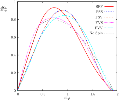
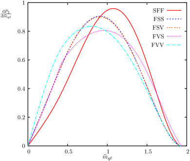
Figure 2: Invariant mass distributions for SPS 1a: Process 1 (top) and Process 2 (bottom).

Figures 3 and 4 show the same distributions for the five spin assignments, for the SPS 2 and SPS 9 mass spectra.

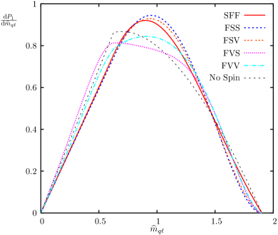
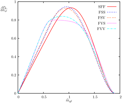
Figure 3: Invariant mass distributions for SPS 2: Process 1 (top) and Process 2 (bottom).

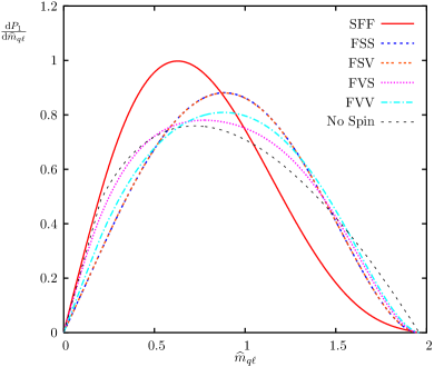
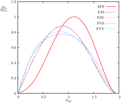
Figure 4: Invariant mass distributions for SPS 9: Process 1 (top) and Process 2 (bottom).

These plots show that all the curves have a similar overall shape, but with some differences due to the different Lorentz structure. The exact effect can be seen in the equations in appendix A. However, quantitative statements can be made. For example, the SFF (MSSM) curve peaks slightly to the left (right) of the others in Process 1 (2) for all mass spectra, although to different degrees. Also, the FSS and FSV curves are very similar particularly at SPS 1a and 9.

From these curves for processes 1 and 2, we can construct the distribution of processes through a $W^{-}$ and the distribution of processes through a $W^{+}$, which are the distributions which would actually be observed. If an $\ell^{-}$ is observed, the chain must have started with the partner of either a down-type quark, or an up-type antiquark. We define $r_{d^{*}}=1-r_{\bar{u}^{*}}$ to be the fraction of chains with an $\ell^{-}$ which begin with the partner of a down-type quark. Similarly, we define $r_{u^{*}}=1-r_{\bar{d}^{*}}$ to be the fraction of chains with an $\ell^{+}$ which begin with the partner of an up-type quark. The $q\ell^{\mp}$ distributions, $\mathrm{d}P_{\mp}/\mathrm{d}\widehat{m}$, are given by:

$$\frac{\mathrm{d}P_{-}}{\mathrm{d}\widehat{m}} = r_{d^{*}}\frac{\mathrm{d}P_{1}}{\mathrm{d}\widehat{m}}+r_{\bar{u}^{*}}\frac{\mathrm{d}P_{2}}{\mathrm{d}\widehat{m}}$$

$$\frac{\mathrm{d}P_{+}}{\mathrm{d}\widehat{m}} = r_{u^{*}}\frac{\mathrm{d}P_{2}}{\mathrm{d}\widehat{m}}+r_{\bar{d}^{*}}\frac{\mathrm{d}P_{1}}{\mathrm{d}\widehat{m}}.$$ (3)

No distinction between flavours of quarks was required in the earlier studies Barr:2004ze ; Smillie:2005ar ; Datta:2005zs ; Athanasiou:2006ef of the cascade decay of a quark partner. In these the quark partner decayed straight into a quark and a neutral particle so no charge information of the original quark was transmitted to the rest of the chain making the results flavour independent.

The MSSM scenarios in table 2 imply the values of the fractions in table 3 at the LHC, i.e. in $pp$ collisions at 14 TeV. Therefore these values represent studying models with the MSSM flavour structure but different spin assignments. We see that at SPS 9, the effect of having more up quarks than down quarks in the proton is dwarfed by the latter’s larger branching ratio to a chargino. This is caused by the large value of the MSSM parameter $\mu$ enhancing the effect of large $\tan\beta$ in the chargino mixing matrices. The resulting plots are shown in figures 5 – 7.

Spectrum	$r_{d^{*}}$	$r_{\bar{u}^{*}}$	$r_{u^{*}}$	$r_{\bar{d}^{*}}$
SPS 1a	0.860	0.140	0.469	0.531
SPS 2	0.900	0.100	0.911	0.089
SPS 9	0.998	0.002	0.072	0.928

Table 3: Numerical calculation of fractions using Herwig.

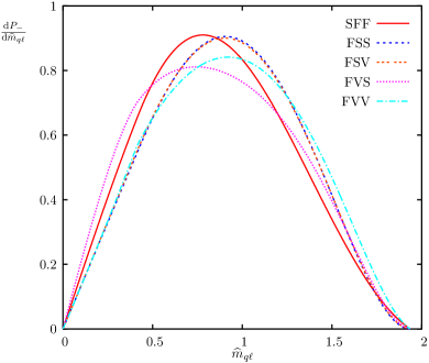
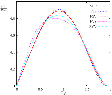
Figure 5: Observable invariant mass distributions for SPS 1a: $P_{-}$ (top) and $P_{+}$ (bottom), see equation (3).

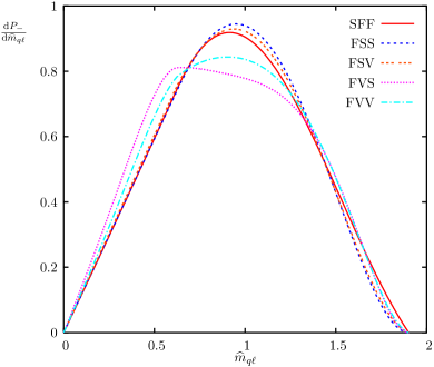
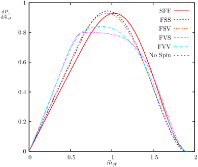
Figure 6: Observable invariant mass distributions for SPS 2: $P_{-}$ (top) and $P_{+}$ (bottom)), see equation (3).

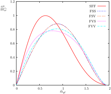
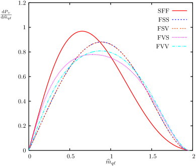
Figure 7: Observable invariant mass distributions for SPS 9: $P_{-}$ (top) and $P_{+}$ (bottom)), see equation (3).

We see that at SPS 9 the plots are nearly identical due to the extreme values of $r_{d^{*}}$ and $r_{\bar{d}^{*}}$ there. There is greater variation in the individual curves at SPS 9 than for the other two mass spectra. Our ability to distinguish the curves is discussed in section 4.

We combine the information from both chains together by forming the asymmetry of the normalised distributions given by

$$A^{\mp}=\frac{\phantom{d}\frac{\mathrm{d}P_{-}}{\mathrm{d}\widehat{m}^{2}}-\frac{\mathrm{d}P_{+}}{\mathrm{d}\widehat{m}^{2}}\phantom{d}}{\frac{\mathrm{d}P_{-}}{\mathrm{d}\widehat{m}^{2}}+\frac{\mathrm{d}P_{+}}{\mathrm{d}\widehat{m}^{2}}}.$$ (4)

The resulting plots are given in figure 8.

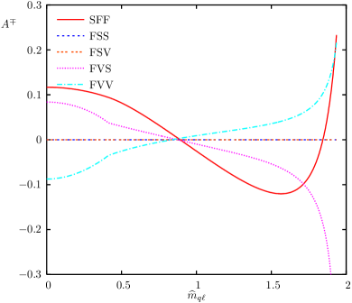
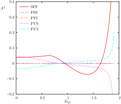
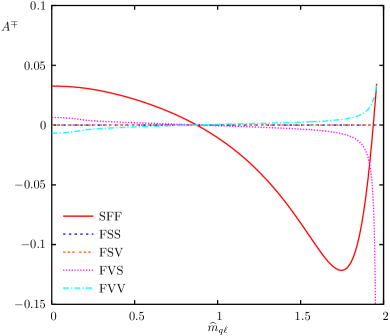
Figure 8: Asymmetry plots for SPS 1a (top), SPS 2 (middle) and SPS 9 (bottom).

The asymmetry at SPS 1a (figure 8, top) shows a difference in the behaviour of the SFF, FVS and FVV curves. With a 10% level of asymmetry, we can be optimistic about distinguishing the SFF (MSSM) curve. The differences at very high and low $\widehat{m}$ cannot usually be used as this is where experimental statistics are often much worse.

In the asymmetry plot for SPS 2 (figure 8, middle), it is unlikely that we would be able to distinguish the FVS and FVV curves from the FSS and FSV line of zero asymmetry. The SFF line peaks at below 10% making it also difficult to observe.

The same plot for SPS 9 (figure 8, bottom) shows low levels of asymmetry for all the curves, with the exception of the SFF curve. Its peak of over 10% asymmetry suggests that for these masses it could be picked out. It is unlikely that any of the other curves could be distinguished from each other for any of these mass spectra.

4 Model discrimination

Here we apply the Kullback-Leibler distance Kullback:1951 . In our notation, it is defined as

$$\mathrm{KL}(T,S)=\int_{m}\log\left(\frac{p(m|T)}{p(m|S)}\right)p(m|T)\,\mathrm{d}m,$$ (5)

where $p(m|T)$ is the probability density function for $m$ given the distribution $T$, and analogously for $p(m|S)$. The expression that distribution $T$ is $R$ times more likely than distribution $S$, on the basis of the data points $\{m_{i}\}$, is

$$R=\frac{p(T|\{m_{i}\})}{p(S|\{m_{i}\})}.$$ (6)

It was shown in Athanasiou:2006ef that this can be rearranged to give a minimum number of events, $N$, needed such that distribution $T$ is calculated to be $R$ times more likely than distribution $S$, assuming that $T$ is the true distribution:

$$N\sim\frac{\log R+\log\frac{p(S)}{p(T)}}{\mathrm{KL}(T,S)}$$ (7)

in the limit $N\gg 1$ where $p(S)$ and $p(T)$ are the prior probabilities of each distribution. We must make an assumption about the true distribution as we must generate our data points for comparison from a particular distribution. This will not be the case when we have real data. We include the factor $\log($$p(S)/p(T)$$)$ for completeness, however, we will set it to zero in our analysis. This is equivalent to assuming all distributions to be equally likely before we look at the data. Also, as pointed out in Athanasiou:2006ef , the result is invariant under diffeomorphisms $m\to f(m)$, so the result would be unaffected if we had calculated with functions of $\widehat{m}^{2}$ for example, instead of $\widehat{m}$.

The value $N$ is an absolute lower bound on the required number of events. Once background and detector effects are included these will rise considerably, however, these effects vary from experiment to experiment and hence it is useful to have a universal lower bound.

The results for the observable $P_{\mp}$ distributions at SPS 1a (figure 5) are given in table 4. The corresponding results for the curves at SPS 2 (figure 6) and SPS 9 (figure 7) are shown in tables 5 and 6. The value $R=1000$ has been taken here, so we are asking for one model to appear 1000 times more likely than another. This corresponds to a 99.9% confidence level, but is a matter of choice.

(a)	SFF	FSS	FSV	FVS	FVV
SFF	$\infty$	697	756	1237	468
FSS	712	$\infty$	177273	464	1481
FSV	764	171080	$\infty$	498	1687
FVS	1221	434	466	$\infty$	444
FVV	448	1298	1512	465	$\infty$

(b)	SFF	FSS	FSV	FVS	FVV
SFF	$\infty$	6728	9459	975	2801
FSS	7728	$\infty$	177273	732	1689
FSV	10408	171080	$\infty$	819	2022
FVS	938	688	778	$\infty$	5523
FVV	2734	1590	1932	5605	$\infty$

Table 4: Number of events needed, with SPS 1a masses, to disfavour the column model with respect to the row model by a factor of 1/1000, assuming the data to come from the row model, for (a) $\mathrm{d}P_{-}/\mathrm{d}\widehat{m}$ and (b) $\mathrm{d}P_{+}/\mathrm{d}\widehat{m}$.

(a)	SFF	FSS	FSV	FVS	FVV
SFF	$\infty$	1220	2223	704	2166
FSS	1608	$\infty$	19314	570	1292
FSV	2668	17780	$\infty$	738	2047
FVS	721	560	730	$\infty$	3181
FVV	2267	1240	2016	3211	$\infty$

(b)	SFF	FSS	FSV	FVS	FVV
SFF	$\infty$	1484	1468	586	649
FSS	1531	$\infty$	19314	639	1106
FSV	1483	17780	$\infty$	853	1655
FVS	572	619	840	$\infty$	5551
FVV	630	1081	1638	5660	$\infty$

Table 5: As in table 4 for the SPS 2 mass spectrum, for (a) $\mathrm{d}P_{-}/\mathrm{d}\widehat{m}$ and (b) $\mathrm{d}P_{+}/\mathrm{d}\widehat{m}$.

(a)	SFF	FSS	FSV	FVS	FVV
SFF	$\infty$	90	90	118	87
FSS	83	$\infty$	5939353	648	1686
FSV	83	5888890	$\infty$	659	1734
FVS	97	608	618	$\infty$	1780
FVV	73	1605	1654	1844	$\infty$

(b)	SFF	FSS	FSV	FVS	FVV
SFF	$\infty$	123	124	162	121
FSS	117	$\infty$	5939353	666	1686
FSV	118	5888890	$\infty$	677	1735
FVS	139	626	637	$\infty$	2176
FVV	105	1609	1659	2253	$\infty$

Table 6: As in table 4 for the SPS 9 mass spectrum, for (a) $\mathrm{d}P_{-}/\mathrm{d}\widehat{m}$ and (b) $\mathrm{d}P_{+}/\mathrm{d}\widehat{m}$.

The lower numbers in the SPS 9 tables reflect the original impression from the graphs that the curves are easier to separate at this point than at SPS 1a or 2. The exception is between the FSS and FSV curves, which was to be expected from the similar functional form. The values for SFF (which corresponds to the MSSM) are the lowest, but are still of the order of 100. These will be degraded in an experimental situation.

The numbers in tables 4 – 6 treat the $W^{+}$ and $W^{-}$ chains individually, however, we can reasonably expect that if one is observed, both will be. The relative numbers of the two chains again depend on the masses in the chain. With experimental data these values would be known, but here we rely on the MSSM values obtained in the same way as those in table 3. The results are shown in table 7, where the fraction of $W$ chains which included a $W^{\pm}$ is denoted $f_{\pm}$.

When we consider both sets of data at once, equation (5) is generalised to

$${\rm KL}(T,S)\; = \;\int_{m}\log\left(\frac{p(m^{+}|T^{+})}{p(m^{+}|S^{+})}\right)p(m^{+}|T^{+})$$ (8)

$$\quad+\log\left(\frac{p(m^{-}|T^{-})}{p(m^{-}|S^{-})}\right)p(m^{-}|T^{-})\;\mathrm{d}m$$

$$= \quad\>\>{\rm KL}^{+}(T,S)\quad+\quad{\rm KL}^{-}(T,S)$$

where $p(m^{\pm}|U^{\pm})=f_{\pm}\;p(m|U^{\pm})$. This gives the values of $N$ shown in table 8.

Spectrum	$f_{+}$	$f_{-}$
SPS 1a	0.57	0.43
SPS 2	0.68	0.32
SPS 9	0.67	0.33

Table 7: Fractions, $f_{\pm}$, of total number of $W$ chains which include a $W^{\pm}$ for each mass spectrum.

(a)	SFF	FSS	FSV	FVS	FVV
SFF	$\infty$	1425	1589	1073	891
FSS	1476	$\infty$	1.8$\cdot 10^{5}$	587	1593
FSV	1619	1.8$\cdot 10^{5}$	$\infty$	642	1863
FVS	1041	549	604	$\infty$	933
FVV	855	1450	1726	975	$\infty$

(b)	SFF	FSS	FSV	FVS	FVV
SFF	$\infty$	1388	1647	619	837
FSS	1554	$\infty$	1.9$\cdot 10^{4}$	615	1160
FSV	1729	1.8$\cdot 10^{4}$	$\infty$	812	1763
FVS	613	599	801	$\infty$	4482
FVV	819	1127	1742	4550	$\infty$

(c)	SFF	FSS	FSV	FVS	FVV
SFF	$\infty$	110	110	144	107
FSS	103	$\infty$	5.9$\cdot 10^{6}$	660	1686
FSV	103	5.9$\cdot 10^{6}$	$\infty$	671	1734
FVS	122	620	631	$\infty$	2027
FVV	92	1607	1657	2100	$\infty$

Table 8: Total number of $W^{+}$ and $W^{-}$ events needed to disfavour the column model with respect to the row model by factor of 1/1000, assuming data to come from the row model at (a) SPS 1a, (b) SPS 2 and (c) SPS 9.

In order to illustrate how these numbers show an improvement over treating the distributions separately, we consider the specific values of the (SFF,FVS) entry at SPS 9. For the $P_{-}$ distribution alone it was 118, while for $P_{+}$ alone it was 162. For this mass spectrum, a third of the chains have a $W^{-}$. This means that looking at the whole sample, for every $W^{-}$ event there are roughly two $W^{+}$ events. If the $W^{+}$ events contributed no discriminatory information (that is if $p(m^{+}|{\rm SFF})=p(m^{+}|{\rm FVS})$ for all $m^{+}$), then we would expect to need about $3$ times the number of $W^{-}$ events alone, 354. However, as the $W^{+}$ events do contribute to distinguishing the two models, we find that only 144 events in total are required.

Equation (7) shows that when the prior probabilities of the models are equal (i.e. $p(S)=p(T)$ as we have used) the number of events $N_{1}$ calculated for a discrimination level $R=R_{1}$ is related to the number of events $N_{2}$ calculated with $R=R_{2}$ by a multiplicative factor. For example, to obtain the results for $R=20$ (which corresponds to a 95% confidence level), the numbers in table 4 should be multiplied by $\log(20)/\log(1000)\simeq 0.43$.

It is instructive to consider how these events translate into required luminosity. The cross sections for these chains in the MSSM are given in table 9, where the branching ratios of $\chi^{\pm}_{2}\to W$ and $W\to e,\mu$ have been taken into account. This corresponds to considering the first row in each table — that in which the MSSM is the true scenario. The quoted required luminosity is calculated using the maximum number which appears in the first row of each table.

Spectrum	Cross Section (fb)	Luminosity (fb-1)
SPS 1a	12.3	129
SPS 2	1.41	1171
SPS 9	0.03	5473

Table 9: Cross sections for chains of the form shown in figure 1 in the MSSM and corresponding integrated luminosity.

The highest cross section is for the SPS 1a mass spectrum, which is as expected as it is relatively light. This gives a required luminosity of 129 fb^-1. The design integrated luminosity for the LHC is 300 fb^-1, before upgrade. This is encouraging, however, the required value will inevitably increase when detector and background effects are considered. It looks unlikely that these studies could be conducted at this level of discrimination for either SPS 2 or SPS 9. The effect of the low numbers at SPS 9 has been suppressed by the small branching ratio of $\widetilde{q}_{L}\to q_{L}^{\prime}\widetilde{\chi}^{\pm}_{2}$ at this point.

5 Conclusions

The spin correlations in the decay of a quark partner via a leptonic $W$ boson decay, as exhibited in the invariant mass distributions of the quark and charged lepton, have been studied for three distinct SUSY-inspired mass spectra (SPS points 1a, 2 and 9). We have considered the 5 possible spin assignments in the chain and studied the extent to which they can be distinguished. The observable invariant mass distributions were constructed where we found that the distributions had similar functional form. The asymmetry constructed from these plots could be useful for distinguishing the SFF curve (which corresponds to the MSSM) from any of the other curves, but depends on the mass spectrum.

The results were quantified using the Kullback-Leibler distance to give a lower bound on the number of events required to distinguish the spin assignments at a given level of certainty. This was applied to the distributions individually, and then to them combined. These provide a guide to how useful particular channels would be in a study like this. The lowest numbers were for the SPS 9 mass spectrum where the lower bound was of the order of 100 events when attempting to distinguish the SFF curve from others, and higher (in some cases considerably) when attempting to distinguish between the other distributions. It therefore seems that this could be a useful method to distinguish the MSSM from other spin assignments in the chain, but will be less useful to distinguish amongst these alternatives.

These bounds were converted to a luminosity requirement for the case where the MSSM was the true scenario. The values for the SPS 1a mass spectrum were encouraging, while for SPS 2 and SPS 9 it appears unlikely that this method could give a high level of discrimination.

Appendix A Analytical formulae

This section contains the formulae for the distributions plotted in section 3 (with the exception of FVV, see below). They are expressed in terms of two constants $k_{1}$ and $k_{2}$ which are functions of the mass ratios described in section 3:

$$k_{1}=1+Y-Z\qquad\mathrm{and}\qquad k_{2}=\sqrt{k_{1}^{2}-4Y},$$ (9)

such that $k_{1}>k_{2}>0$. Then equations (1) and (2) give

$$\widehat{m}^{2}_{q\ell} = k_{1}(1-\cos\theta\cos\psi)+k_{2}(\cos\theta-\cos\psi)$$ (10)

$$\quad-2\sqrt{Y}\sin\theta\sin\psi\cos\phi$$

with maximum $2(k_{1}+k_{2})$. We define the shorthands $k_{12}^{\pm}=k_{1}\pm k_{2}$ and $\widehat{m}=\widehat{m}_{q\ell}$.

Each distribution has different behaviour in the regions $0\leq\widehat{m}^{2}\leq 2k_{12}^{-}$ and $2k_{12}^{-}\leq\widehat{m}^{2}\leq 2k_{12}^{+}$, as can be seen in figures 2 – 4 and in the equations below. This is because high values of $\widehat{m}^{2}$ can only occur for very specific angle configurations which cuts down the phase space and leads to logarithmic behaviour. This can be seen in the “No spin” curve in figures 2(top), 3(top) and 4(top) which represents the phase space. Without this effect, the “No Spin” distribution would continue linearly in $\widehat{m}^{2}\geq 2k_{12}^{-}$.

SFF

In the MSSM, the structure of the $B$-$W$-$A$ vertex is $1+\alpha\gamma_{5}$ where $\alpha$ is defined by the parameters of the model. As this varies at each mass point, it is left explicitly in the equations below. Table 10 lists the values of $\alpha$ at the particular points studied in this paper.

Mass Spectrum	SPS 1a	SPS 2	SPS 9
$\alpha$	0.5083	0.3875	0.8155

Table 10: Numerical values of the parameter $\alpha$ for the different mass spectra studied in the text.

$$\frac{\mathrm{d}P_{1}}{\mathrm{d}\widehat{m}} = \frac{3\widehat{m}}{32k_{2}((1+\alpha^{2})(k_{1}^{2}+2Y-3k_{1}Y)-6Y\sqrt{Z}(1-\alpha^{2}))}$$ (26)

$$\;\times\left\{\begin{array}[]{l@{}l}16\left(k_{2}((1+\alpha)^{2}k_{1}+4(1+\alpha)^{2}Y\phantom{\frac{k_{1}}{k_{2}}}\right.&\\ \quad+\widehat{m}^{2}(1+4\alpha+\alpha^{2}+(-1+\alpha^{2})\sqrt{Z}))&\\ \quad-(2\alpha k_{1}\widehat{m}^{2}+(2(1+\alpha)^{2}(1+k_{1})&\\ \quad\left.+(1+\alpha^{2})\widehat{m}^{2})Y)\log{\left(\frac{k_{1}+k_{2}}{k_{1}-k_{2}}\right)}\right)&\\ \qquad\qquad\qquad\qquad\qquad\qquad 0\leq\widehat{m}^{2}\leq 2k_{12}^{-}\\ &\\ 8k_{1}^{2}(1+\alpha)^{2}+(1+(-6+\alpha)\alpha)\widehat{m}^{4}\\ \quad+8k_{1}((1+\alpha)^{2}(k_{2}+4Y)&\\ \quad+\widehat{m}^{2}(-2-\alpha(2+\alpha(2+\sqrt{Z}))+\sqrt{Z}))\\ \quad+8\widehat{m}^{2}(-2(1+\alpha)^{2}Y+k_{2}(1+4\alpha+\alpha^{2}&\\ \quad-(1-\alpha^{2})\sqrt{Z}))+16Y((1+\alpha)^{2}(5+2k_{2})&\\ \quad-4(1-\alpha^{2})\sqrt{Z})-16(2\alpha k_{1}\widehat{m}^{2}\\ \quad+(2(1+\alpha)^{2}(1+k_{1})&\\ \quad+(1+\alpha^{2})\widehat{m}^{2})Y)\log{\left(\frac{2(k_{1}+k_{2})}{\widehat{m}^{2}}\right)}&\\ \qquad\qquad\qquad\qquad\qquad\qquad 2k_{12}^{-}\leq\widehat{m}^{2}\leq 2k_{12}^{+}&\\ \end{array}\right.$$

$$\frac{\mathrm{d}P_{2}}{\mathrm{d}\widehat{m}} = \frac{3\widehat{m}}{32k_{2}((1+\alpha^{2})(k_{1}^{2}+2Y-3k_{1}Y)-6Y\sqrt{Z}(1-\alpha^{2}))}$$ (42)

$$\;\times\left\{\begin{array}[]{l@{}l}-16\left(k_{2}(\widehat{m}^{2}+4Y-k_{1}(1-\alpha)^{2}\phantom{\frac{k_{1}}{k_{2}}}\right.&\\ \quad+\alpha(\widehat{m}^{2}(4+\alpha)+4\alpha Y)-\widehat{m}^{2}\sqrt{Z}(1-\alpha^{2}))\\ \quad-(Y(2+\widehat{m}^{2}-4\sqrt{Z})+2\alpha(k_{1}\widehat{m}^{2}+2Y)\\ \quad\left.+Y(2+\widehat{m}^{2}+4\sqrt{Z})\alpha^{2})\log{\left(\frac{k_{1}+k_{2}}{k_{1}-k_{2}}\right)}\right)&\\ \qquad\qquad\qquad\qquad\qquad\qquad 0\leq\widehat{m}^{2}\leq 2k_{12}^{-}\\ &\\ 8k_{1}^{2}(1-\alpha)^{2}+\widehat{m}^{4}(1+\alpha(6+\alpha))&\\ \quad-16Y(3+2k_{2}-4\sqrt{Z}&\\ \quad+\alpha(10+\alpha(3+2k_{2}+4\sqrt{Z})))&\\ \quad+8k_{1}(k_{2}(1-\alpha)^{2}+2\widehat{m}^{2}\alpha-\widehat{m}^{2}\sqrt{Z}(1-\alpha^{2})\\ \quad-4Y(1+\alpha^{2}))-8\widehat{m}^{2}(-2Y(1+\alpha^{2})\\ \quad+k_{2}(1+4\alpha+\alpha^{2}+\sqrt{Z}(-1+\alpha^{2})))\\ \quad+16(Y(2+\widehat{m}^{2}-4\sqrt{Z})+2\alpha(k_{1}\widehat{m}^{2}+2Y)\\ \quad+\alpha^{2}Y(2+\widehat{m}^{2}+4\sqrt{Z}))\log{\left(\frac{2(k_{1}+k_{2})}{\widehat{m}^{2}}\right)}&\\ \qquad\qquad\qquad\qquad\qquad\qquad 2k_{12}^{-}\leq\widehat{m}^{2}\leq 2k_{12}^{+}\\ \end{array}\right.$$

FSS

$$\frac{\mathrm{d}P_{1,2}}{\mathrm{d}\widehat{m}} = \frac{3\widehat{m}}{2k_{2}^{3}}\left\{\begin{array}[]{l l}k_{1}k_{2}-2Y\log\left(\frac{k_{1}+k_{2}}{k_{1}-k_{2}}\right)&\\ \qquad\qquad\qquad\qquad\qquad 0\leq\widehat{m}^{2}\leq 2k_{12}^{-}\\ &\\ \frac{1}{16}(6k_{1}-2k_{2}-\widehat{m}^{2})(2(k_{1}+k_{2})-\widehat{m}^{2})&\\ -2Y\log\left(\frac{2(k_{1}+k_{2})}{\widehat{m}^{2}}\right)&\\ \qquad\qquad\qquad\qquad\qquad 2k_{12}^{-}\leq\widehat{m}^{2}\leq 2k_{12}^{+}\\ \end{array}\right.$$ (49)

FSV

$$\frac{\mathrm{d}P_{1,2}}{\mathrm{d}\widehat{m}} = \frac{3\widehat{m}}{2k_{2}(k_{2}^{2}+12YZ)}$$ (56)

$$\times\left\{\begin{array}[]{l c}k_{1}k_{2}+2Y(2Z-1)\log\left(\frac{k_{1}+k_{2}}{k_{1}-k_{2}}\right)&\\ \qquad\qquad\qquad\qquad\qquad 0\leq\widehat{m}^{2}\leq 2k_{12}^{-}\\ &\\ \frac{1}{16}(6k_{1}-2k_{2}-\widehat{m}^{2})(2(k_{1}+k_{2})-\widehat{m}^{2})&\\ \quad+2Y(2Z-1)\log\left(\frac{2(k_{1}+k_{2})}{\widehat{m}^{2}}\right)&\\ \qquad\qquad\qquad\qquad\qquad 2k_{12}^{-}\leq\widehat{m}^{2}\leq 2k_{12}^{+}\end{array}\right.$$

FVS

For the FVS chain the parameter $a$ represents that in the $C$-$q$-$B$ vertex, discussed at the end of section 2.

$$\frac{\mathrm{d}P_{1}}{\mathrm{d}\widehat{m}} = \frac{9\widehat{m}(k_{1}+k_{2})^{2}}{8k_{2}(1+a^{2})(1+2X)(k_{1}(k_{1}+k_{2})-2Y)(k_{1}^{2}+8Y)}$$ (71)

$$\times\left\{\begin{array}[]{l c}2k_{2}(1+a^{2})(k_{1}+6\widehat{m}^{2})&\\ \quad-4Xk_{2}\widehat{m}^{2}(3+a(3a-2))&\\ \quad+(\widehat{m}^{2}(1+a^{2})(4k_{1}+\widehat{m}^{2})(-1+X)&\\ \quad-4Y(1+a^{2}-2X(1-a)^{2}))\log\left(\frac{k_{1}+k_{2}}{k_{1}-k_{2}}\right)&\\ \qquad\qquad\qquad\qquad\qquad\qquad 0\leq\widehat{m}^{2}\leq 2k_{12}^{-}\\ &\\ \frac{1}{8}\left(\left(2(2(k_{1}+k_{2})-\widehat{m}^{2})((1+a^{2})k_{2}(k_{1}+k_{2})\right.\phantom{\frac{k_{1}}{k_{2}}}\right.&\\ \quad\times(4k_{2}+\widehat{m}^{2}(15-16X))&\\ \quad-2(-(1+a^{2})(22k_{1}+26k_{2}+15\widehat{m}^{2})&\\ \quad+16((1-a)^{2}(k_{1}+k_{2})&\\ \quad\left.+(1+a^{2})\widehat{m}^{2})X)Y)\right)/(k_{1}+k_{2})^{2}&\\ \quad+8((1+a^{2})\widehat{m}^{2}(4k_{1}+\widehat{m}^{2})(-1+X)&\\ \quad\left.-4Y(1+a^{2}-2X(1-a)^{2}))\log\left(\frac{2(k_{1}+k_{2})}{\widehat{m}^{2}}\right)\right)&\\ \qquad\qquad\qquad\qquad\qquad\qquad 2k_{12}^{-}\leq\widehat{m}^{2}\leq 2k_{12}^{+}\\ \end{array}\right.$$

$$\frac{\mathrm{d}P_{2}}{\mathrm{d}\widehat{m}} = \frac{\mathrm{d}P_{1}}{\mathrm{d}\widehat{m}}\quad\mathrm{with}\quad a\to-a$$ (72)

FVV

The FVV distributions are too long to present here in a manageable way due to the complicated $B^{\pm}$–$W^{\pm}$–$A$ vertex. They are available on request from the author. They also have the symmetry (72).

Appendix B Higher dimensional couplings

As mentioned in section 2, this analysis did not consider higher dimensional couplings with a different Lorentz structure to that considered previously in the paper. For example, vertices with the form (a) $p.qg^{\mu\nu}-p^{\nu}q^{\mu}$ or (b) $\epsilon^{\mu\nu\rho\sigma}p_{\rho}q_{\sigma}$ are studied in the context of anomalous Higgs couplings Hankele:2006ma .

Figure 9 shows the distributions for the FSV chain with these different vertices alongside the distribution shown before (marked FSV), for the SPS 1a mass spectrum.

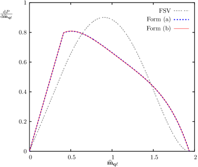
Figure 9: Distributions for the different scalar-vector-vector vertices described in the text.

The new vertices give very similar distributions; the analytical expressions are given below. Due to the scalar in the chain the distributions for processes 1 and 2 are the same and therefore so are the distributions for the chains with positive and negative leptons.

$$\frac{\mathrm{d}P_{\mathrm{(a)}}}{\mathrm{d}\widehat{m}} = \frac{3\widehat{m}}{4k_{2}(k_{2}^{2}+6YZ)}$$ (79)

$$\times\left\{\begin{array}[]{l c}-k_{1}k_{2}+((k_{1}-2Y)^{2}+2Y)\log\left(\frac{k_{1}+k_{2}}{k_{1}-k_{2}}\right)&\\ \qquad\qquad\qquad\qquad\qquad\qquad 0\leq\widehat{m}^{2}\leq 2k_{12}^{-}\\ &\\ \frac{1}{16}\left(-(6k_{1}-2k_{2}-\widehat{m})(2(k_{1}+k_{2})-\widehat{m})\phantom{\frac{2(k_{1})}{2}}\right.&\\ \left.\quad+16((k_{1}-2Y)^{2}+2Y)\log\left(\frac{2(k_{1}+k_{2})}{\widehat{m}^{2}}\right)\right)&\\ \qquad\qquad\qquad\qquad\qquad\qquad 2k_{12}^{-}\leq\widehat{m}^{2}\leq 2k_{12}^{+}\end{array}\right.$$

$$\frac{\mathrm{d}P_{\mathrm{(b)}}}{\mathrm{d}\widehat{m}} = \frac{3\widehat{m}}{4k_{2}^{3}}\left\{\begin{array}[]{l}-k_{1}k_{2}+(k_{1}^{2}-2Y)\log\left(\frac{k_{1}+k_{2}}{k_{1}-k_{2}}\right)\\ \qquad\qquad\qquad\qquad 0\leq\widehat{m}^{2}\leq 2k_{12}^{-}\\ \\ \frac{1}{16}\left(-(6k_{1}-2k_{2}-\widehat{m}^{2})\phantom{\frac{2(k_{1})}{2}}\right.\\ \quad\times(2(k_{1}+k_{2})-\widehat{m}^{2})\\ \left.\quad+16(k_{1}^{2}-2Y)\log\left(\frac{2(k_{1}+k_{2})}{\widehat{m}^{2}}\right)\right)\\ \qquad\qquad\qquad\qquad 2k_{12}^{-}\leq\widehat{m}^{2}\leq 2k_{12}^{+}\end{array}\right.$$ (87)

While the distributions are very similar to each other, they are quite different to that of the same chain with the lowest order vertex and to the distributions for the other chains shown in figure 5. Therefore vertices of this kind would be unlikely to be mistaken for those already discussed.

References

- (1) T. Appelquist, H.-C. Cheng, and B. A. Dobrescu, “Bounds on universal extra dimensions,” Phys. Rev. D64 (2001) 035002, hep-ph/0012100.
- (2) N. Arkani-Hamed, A. G. Cohen, and H. Georgi, “Electroweak symmetry breaking from dimensional deconstruction,” Phys. Lett. B513 (2001) 232–240, hep-ph/0105239.
- (3) A. J. Barr, “Using lepton charge asymmetry to investigate the spin of supersymmetric particles at the LHC,” Phys. Lett. B596 (2004) 205–212, hep-ph/0405052.
- (4) T. Goto, K. Kawagoe, and M. M. Nojiri, “Study of the slepton non-universality at the CERN Large Hadron Collider,” Phys. Rev. D70 (2004) 075016, hep-ph/0406317.
- (5) J. M. Smillie and B. R. Webber, “Distinguishing spins in supersymmetric and universal extra dimension models at the Large Hadron Collider,” JHEP 10 (2005) 069, hep-ph/0507170.
- (6) M. Battaglia, A. Datta, A. De Roeck, K. Kong, and K. T. Matchev, “Contrasting supersymmetry and universal extra dimensions at the CLIC multi-TeV e+ e- collider,” JHEP 07 (2005) 033, hep-ph/0502041.
- (7) A. Datta, K. Kong, and K. T. Matchev, “Discrimination of supersymmetry and universal extra dimensions at hadron colliders,” Phys. Rev. D72 (2005) 096006, hep-ph/0509246.
- (8) A. Datta, G. L. Kane, and M. Toharia, “Is it SUSY?,” hep-ph/0510204.
- (9) A. J. Barr, “Measuring slepton spin at the LHC,” JHEP 02 (2006) 042, hep-ph/0511115.
- (10) A. Alves, O. Eboli, and T. Plehn, “It’s a gluino,” hep-ph/0605067.
- (11) H.-C. Cheng, K. T. Matchev, and M. Schmaltz, “Bosonic supersymmetry? getting fooled at the LHC,” Phys. Rev. D66 (2002) 056006, hep-ph/0205314.
- (12) C. Athanasiou, C. G. Lester, J. M. Smillie, and B. R. Webber, “Distinguishing spins in decay chains at the large hadron collider,” JHEP 06 (2006) 082, hep-ph/0605286.
- (13) P. Meade and M. Reece, “Top partners at the LHC: Spin and mass measurement,” hep-ph/0601124.
- (14) L.-T. Wang and I. Yavin, “Spin measurements in cascade decays at the LHC,” hep-ph/0605296.
- (15) H.-C. Cheng and I. Low, “Little hierarchy, little Higgses, and a little symmetry,” JHEP 08 (2004) 061, hep-ph/0405243.
- (16) H.-C. Cheng, K. T. Matchev, and M. Schmaltz, “Radiative corrections to Kaluza-Klein masses,” Phys. Rev. D66 (2002) 036005, hep-ph/0204342.
- (17) B. C. Allanach et al., “The Snowmass points and slopes: Benchmarks for SUSY searches,” Eur. Phys. J. C25 (2002) 113–123, hep-ph/0202233.
- (18) G. Corcella et al., “HERWIG 6: An event generator for hadron emission reactions with interfering gluons (including supersymmetric processes),” JHEP 01 (2001) 010, hep-ph/0011363.
- (19) G. Corcella et al., “HERWIG 6.5 release note,” hep-ph/0210213.
- (20) S. Moretti, K. Odagiri, P. Richardson, M. H. Seymour, and B. R. Webber, “Implementation of supersymmetric processes in the HERWIG event generator,” JHEP 04 (2002) 028, hep-ph/0204123.
- (21) A. D. Martin, R. G. Roberts, W. J. Stirling, and R. S. Thorne, “Scheme dependence, leading order and higher twist studies of MRST partons,” Phys. Lett. B443 (1998) 301–307, hep-ph/9808371.
- (22) S. Kullback and R. A. Leibler, “On information and sufficiency,” Annals of Mathematical Statistics 22(1) (1951) 79–86.
- (23) V. Hankele, G. Klamke, D. Zeppenfeld, and T. Figy, “Anomalous higgs boson couplings in vector boson fusion at the CERN LHC,” Phys. Rev. D74 (2006) 095001, hep-ph/0609075.