Abstract

BES data on the $\sigma$ pole are refitted taking into account new information on coupling of $\sigma$ to $KK$ and $\eta\eta$. The fit also includes Cern-Munich data on $\pi\pi$ elastic phases shifts and $K_{e4}$ data, and gives a pole position of $500\pm 30-i(264\pm 30)$ MeV. There is a clear discrepancy with the $\sigma$ pole position recently predicted by Caprini et al. using the Roy equation. This discrepancy may be explained naturally by uncertainties arising from inelasticity in $KK$ and $\eta\eta$ channels and mixing between $\sigma$ and $f_{0}(980)$. Adding freedom to accomodate these uncertainties gives an optimum compromise with a pole position of $472\pm 30-i(271\pm 30)$ MeV.

PACS: 13.25.-k, 13.75.Lb, 14.40.Cs, 14.40.Ev.

1 Introduction

BES data on $J/\Psi\to\omega\pi^{+}\pi^{-}$ display a conspicuous low mass $\pi\pi$ peak due to the $\sigma$ pole [1]. It was observed less clearly in earlier DM2 [2] and E791 data [3]. The BES data are reproduced in Fig. 1. The band along the upper right-hand edge of the Dalitz plot, Fig. 1(a), is due to the $\sigma$ pole. There is a clear peak in the $\pi\pi$ mass projection of Fig. 1(b) at $\sim 500$ MeV; the fitted $\sigma$ contribution is shown by the full histogram of Fig. 1(d). Other large contributions to the data arise from $f_{2}(1270)$ and $b_{1}(1235)$, which appears in the $\omega\pi$ mass projection of Fig. 1(c).

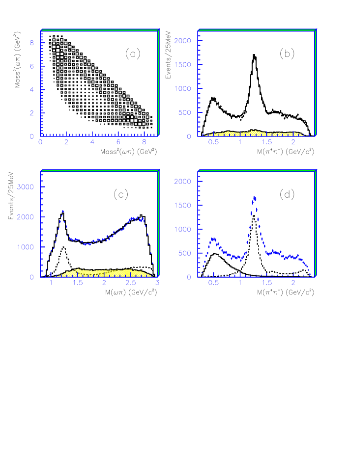
Figure 1: BES data of Ref. [1]. (a) Dalitz plot; (b) $\pi\pi$ mass projection: the upper histogram shows fit (ii) of Table 1, the lower histogram shows experimental background; (c) $\omega\pi$ mass projection; full histograms are as in (b) and the dashed histogram shows the coherent sum of both $b_{1}(1235)\pi$ contributions; (d) $\pi\pi$ mass projections from $\sigma$ (full curve) and spin 2 (dashed).

At the time of the BES analysis, little was known about the coupling of $\sigma$ to $KK$ and $\eta\eta$, and these channels were omitted from the fit to the data. Since then, couplings to $KK$ and $\eta\eta$ have been determined by fitting (a) all available data on $\pi\pi\to KK$ and $\eta\eta$, (b) Kloe and Novosibirsk data on $\phi\to\gamma(\pi^{0}\pi^{0})$ [4]. All these data agree on a substantial coupling of $\sigma$ to $KK$. The first objective of the present work is to refit the $J/\Psi\to\omega\pi\pi$ data including this coupling, following exactly the procedure of the BES publication. The outcome is to move the $\sigma$ pole position from $541\pm 39-i(252\pm 41)$ MeV reported in the BES paper to $500\pm 30-i(264\pm 30)$ MeV.

Meanwhile, Caprini, Colangelo and Leutwyler (denoted hereafter as CCL) have made a prediction of the $\sigma$ pole position [5]. Their calculation is based on the Roy equation for $\pi\pi$ elastic scattering [6], which embodies constraints of analyticity, unitarity and crossing symmetry. This approach has the merit of including driving forces from the left-hand cut due to exchange of $\rho$, $f_{2}$ and $\sigma$. They also apply tight constraints from Chiral Perturbation Theory (ChPT) on the S-wave scattering lengths $a_{0}$ and $a_{2}$ for isospins 0 and 2. Experiment alone determines only the upper side of the pole well; this has led to speculation that fits without a pole might succeed in fitting the data [7]. CCL’s use of crossing symmetry and analyticity gives a precise determination of the magnitude and phase of the S-wave amplitude on the lower side of the pole and leaves no possible doubt about its existence. They clarify the fact that $\pi\pi$ dynamics are fundamental to creating the pole. They quote rather small errors: $M_{\sigma}=441^{+16}_{-8}-i(272^{+9}_{-12.5})$ MeV. There is a rather large discrepancy between this prediction and BES data. A second objective of the present work is to trace the origin of this discrepancy. In outline, what emerges is as follows.

From CCL results for $T_{11}(s)$, the T-matrix for $\pi\pi$ elastic scattering, one can predict what should appear in BES data. The prediction will be shown below on Fig. 4 by the chain curve. From a glance at this figure, one sees a significant disagreement with the experimental points, which are deduced directly from BES data. The questions which arise are as follows:

• (i) are the hypotheses used in the BES analysis wrong or questionable?

• (ii) is something missing from the calculation with the Roy equation?

• (iii) can the calculation of CCL be fine-tuned in order to come into agreement with the experimental data?

The discrepancy lies in the mass range 550 to 950 MeV. In this range, the analysis is sensitive to assumptions about inelasticities due to $KK$ and $\eta\eta$ channels. These are not known with sufficient accuracy at present and allow freedom in the analytic continuation of couplings to these channels below their thresholds. The amplitude for $KK\to\pi\pi$ goes to zero at the $KK$ threshold; it also has an Adler zero at $s\simeq 0.5m_{\pi}^{2}$. In between, it has a peak near 500 MeV providing a natural explanation of the additional peaking required by BES data. This can readily explain the discrepancy, as shown by the full curve on Fig. 4. It may be regarded as a fine-tuning of the solution of the Roy equation. It will be shown that changes to $\pi\pi$ phase shifts up to 750 MeV are $<1.2^{\circ}$, well below experimental errors. In summary, the Roy equation and Chiral Perturbation Theory provide the best description of $\pi\pi$ scattering near threshold (and below), while the BES data provide the best view of the upper side of the $\sigma$ pole.

The layout of the paper is as follows. Section 2 introduces the equations. Section 3 discusses the prediction of CCL and subsection 3.1 explains what is missing from their Roy solution. Section 4 describes fits to BES data. Section 5 discusses possible alternative explanations of BES data and Section 6 summarises conclusions.

2 Equations

The $\pi\pi$ elastic amplitude may be written

$$T_{11}(s)=(\eta e^{2i\delta}-1)/(2i)=N(s)/D(s),$$ (1)

where $N(s)$ is real and describes the left-hand cut; $D(s)$ describes the right-hand cut. The numerator contains an Adler zero at $s=s_{A}\simeq 0.41m^{2}_{\pi}$:

$$N(s)=(s-s_{A})f(s),$$ (2)

where $f(s)$ varies slowly with $s$. The standard relation to the S-matrix is $T_{11}=(S_{11}-1)/2i$; $T_{11}$ has contributions from $f_{0}(980)$, $f_{0}(1370)$ and $f_{0}(1500)$ as well as $\sigma$. For elastic scattering, these contributions are combined by multiplying their S-matrices, to satisfy unitarity; this implies adding phases rather than amplitudes.

In the BES publication, it was shown that their data may be fitted with the same $1/D(s)$ for the $\sigma$ component as $K_{e4}$ data [8] and Cern-Munich data [9] within errors. The phase of the $\pi\pi$ S-wave in BES data has the same variation with $s$ as the $\sigma$ component in elastic scattering within experimental errors of $\sim 3.5^{\circ}$ from 450 to 950 MeV [10]. The BES data may be fitted by an amplitude $\Lambda/D(s)$; here, $\Lambda$ is taken as a constant, since the left-hand cut of $J/\Psi\to\omega\sigma$ is very distant. Possible doubts about this assumption will be discussed later. Channels $\pi\pi$, $KK$, $\eta\eta$ and $4\pi$ will be labelled 1 to 4. The parametrisation of the $\sigma$ is given by

$$T_{11}(s) = M\Gamma_{1}(s)/[M^{2}-s-g^{2}_{1}\frac{s-s_{A}}{M^{2}-s_{A}}z(s)-iM\Gamma_{tot}(s)]$$ (3)

$$M\Gamma_{1}(s) = g^{2}_{1}\frac{s-s_{A}}{M^{2}-s_{A}}\rho_{1}(s)$$ (4)

$$g^{2}_{1}(s) = M(b_{1}+b_{2}s)\exp[-(s-M^{2})/A]$$ (5)

$$j_{1}(s) = \frac{1}{\pi}\left[2+\rho_{1}ln_{e}\left(\frac{1-\rho_{1}}{1+\rho_{1}}\right)\right]$$ (6)

$$z(s) = j_{1}(s)-j_{1}(M^{2})$$ (7)

$$M\Gamma_{2}(s) = 0.6g^{2}_{1}(s)(s/M^{2})\exp(-\alpha|s-4m^{2}_{K}|)\rho_{2}(s)$$ (8)

$$M\Gamma_{3}(s) = 0.2g^{2}_{1}(s)(s/M^{2})\exp(-\alpha|s-4m^{2}_{\eta}|)\rho_{3}(s)$$ (9)

$$M\Gamma_{4}(s) = Mg_{4}\rho_{4\pi}(s)/\rho_{4\pi}(M^{2})$$ (10)

$$\rho_{4\pi}(s) = 1.0/[1+\exp(7.082-2.845s)].$$ (11)

D(s) is the denominator of eqn. (3). Below the $KK$ threshold, $Im~{}D=-N(s)$ and $\tan\delta=-Im~{}D/Re~{}D$, from which one can deduce $D(s)$. Since $D(s)$ is analytic, it is subject to a normalisation uncertainty which is constant within the errors of $T_{11}(s)$, in practice 2-3%.

The function $j_{1}(s)$ is obtained from a dispersion integral over the phase space factor $\rho_{\pi\pi}(s)=\sqrt{1-4m^{2}_{\pi}/s}$. An important point about $z(s)$ is that it is well behaved at $s=0$ and eliminates the singularity in $\rho(s)$. It makes the treatment of the $\pi\pi$ channel fully analytic - an improvement on earlier work. In the $4\pi$ channel, a dispersion integral is in principle required but is small below 1 GeV and can be absorbed into the fit to $g_{1}^{2}(s)$. In eqn. (11), $4\pi$ phase space is approximated empirically by a combination of $\rho\rho$ and $\sigma\sigma$ phase space [11] (with $s$ in GeV²); $\Gamma(4\pi)$ is set to zero for $s<16m^{2}_{\pi}$. The effect of the $4\pi$ channel on the $\sigma$ pole is only 2 MeV and is not an issue.

It is assumed that the Adler zero is a feature of the full $\pi\pi$ amplitude. The factor $(s-s_{A})/(M^{2}-s_{A})$ of eqn. (4) introduces this Adler zero explicitly. Eqn. (5) is an empirical form used earlier in fitting BES data; $b_{1}$, $b_{2}$ and $A$ are fitted constants. The factors $s/M^{2}$ in $\Gamma_{2}$ and $\Gamma_{3}$ of eqns. (8) and (9) approximate the Adler zeros closely at $s=0.5m^{2}_{\pi}$, $0.5m^{2}_{K}$ and $0.5m^{2}_{\eta}$ and remove the square root singularity in $\rho_{2}$ and $\rho_{3}$ of eqns. (8) and (9). The factors 0.6 and 0.2 for $g^{2}_{KK}$ and $g^{2}_{\eta\eta}$ have been fitted to data on $\pi\pi\to KK$ and $\eta\eta$ and on $\phi\to\gamma(\pi^{0}\pi^{0})$ [4]. These fits also determine $\alpha_{KK}=\alpha_{\eta\eta}=1.3$ GeV² above the thresholds.

A detail is that the factor $(s-s_{A})/(M^{2}-s_{A})$ is also used for $\Gamma_{1}$, $\Gamma_{2}$ and $\Gamma_{3}$ of $f_{0}(980)$, $f_{0}(1370)$ and $f_{0}(1500)$. Otherwise, parameters of $f_{0}(980)$ are taken from BES data on $J/\Psi\to\phi\pi^{+}\pi^{-}$ and $\phi K^{+}K^{-}$ [12]. The $f_{0}(1500)$ and $f_{0}(1370)$ are fitted with Flatté formulae and parameters given in Ref. [4]. The combined contribution of $f_{0}(980)$, $f_{0}(1370)$ and $f_{0}(1500)$ to the scattering length is 8%.

An important question is how to parametrise the continuation of $KK\to\pi\pi$ and $\eta\eta\to\pi\pi$ amplitudes below their thresholds, i.e. in K-matrix notation the elements $K_{12}$ and $K_{13}$. They can in principle be determined from dispersion relations for each amplitude. The factors $\rho_{2}$ and $\rho_{3}$ in eqns. (8) and (9) are kinematic factors. Below the thresholds, they are continued analytically as $i\sqrt{4m^{2}_{i}-s}$. If $\rho_{2}$ is factored out of the $KK\to\pi\pi$ amplitude, there is a step at threshold in the imaginary part of the surviving amplitude. This step leads to a cusp in the real part of the amplitude at threshold, i.e. a change of slope in eqns. (8) and (9). An evaluation of the dispersion integral generates a result for the real part of the amplitude below threshold close to an exponential falling as $\exp[-\alpha(4m^{2}_{i}-s)]$.

Figure 2: (a) the magnitude of the $KK\to\pi\pi$ amplitude from Büttiker et al. [13]; the result from my fit to Kloe data (full curve) and the $\sigma$ contribution alone (dashed); (c) fit to Kloe $\phi\to\gamma(\pi^{0}\pi^{0})$ data after background subtraction; (d) contributions from $f_{0}(980)$ (full curve), $\sigma$ (dashed) and interference (dotted).

A calculation of $K_{12}$ has been made along these lines by Büttiker, Descotes-Genon and Moussallam using the Roy equations for $\pi K\to\pi K$ and $\pi\pi\to KK$ [13]. Their result is reproduced in Fig. 2(a). The peak is due to $f_{0}(980)$ and the low mass tail comes from the analytic continuation of $\sigma\to KK$. Using their $K_{12}$ in fitting BES data does lead to effects with the right trend, but not with sufficient accuracy to make a good prediction. They remark that their calculation is uncertain because of discrepancies between available sets of data on $\pi\pi\to KK$. My estimate is that errors of Caprini et al from the dispersion relation are at least a factor 2 too small.

My conclusion is that $K_{12}$ and $K_{13}$ presently need to be fitted empirically. There is however experimental information which helps decide an appropriate parametrisation: data on $\phi\to\gamma(\pi^{0}\pi^{0})$ from Kloe [14]. In Ref. [4], those data are fitted using the standard $KK$ loop model of Achasov and Ivanchenko [15]. Parameters of $f_{0}(980)$ are fixed to those determined by BES data [12]. The fit requires a substantial additional amplitude for $KK\to\pi\pi$ through the $\sigma$. Empirically this contribution is well fitted with the exponential of eqn. (8) with $\alpha=2.1$ GeV^-2 below the $KK$ threshold and an Adler zero at $s=0.5m^{2}_{K}$. [The same $\alpha$ is assumed for $\eta\eta\to\pi\pi$.] Fig. 2(c) reproduces from Ref. [4] the fit to Kloe data; Fig. 2(d) shows the $f_{0}(980)$ and $\sigma$ components and the interference between them. Fig. 2(b) compares my fit with that of Büttiker et al.; the dashed curve shows the $\sigma$ contribution.

3 The Roy solution of CCL

CCL make a prediction of the $\pi\pi\to\pi\pi$ S-wave amplitude and deduce the $\sigma$ pole position from it. The inputs to their calculation are [5,16,17]:
i) the Roy equation, which accounts for both left and right-hand cuts in $\pi\pi$ elastic scattering;
ii) the precise lineshape of $\rho(770)$ from $e^{+}e^{-}\to\pi^{+}\pi^{-}$ data;
iii) predicted value from ChPT for S-wave scattering lengths $a_{0}=(0.220\pm 0.005)m_{\pi}^{-1}$, $a_{2}=(-0.0444\pm 0.0010)m_{\pi}^{-1}$ [17];
iv) the $\pi\pi$ phase shift at 800 MeV with an error of ${}^{+10}_{-4}$ deg;
v) my elasticity parameters $\eta$ above the $KK$ threshold;
vi) minor dispersive corrections for masses above 1.15 GeV, their matching point.
Note that experimental phase shifts are not fitted except for constraint (iv).

CCL have kindly supplied a tabulation of their $T_{11}(s)$. My first step is to reproduce this solution using eqns. (1)–(11). This is simply a fit to their fit, i.e. an explicit algebraic parametrisation.

They do not explicitly separate $\sigma$ and $f_{0}(980)$. This leads to uncertainty in how the $f_{0}(980)$ is being fitted. In the vicinity of the $\sigma$ pole, an issue is the magnitude of the low mass tail of $f_{0}(980)$, which affects what is left as the remaining $\sigma$ amplitude. CCL omit $f_{0}(1370)$ and $f_{0}(1500)$ contributions and $\sigma\to 4\pi$.

The fit shown in column (i) of Table 1 is made in two steps. Firstly a fit to their $f_{0}(980)$ is made from 800 to 1150 MeV. It requires $M=0.970$ GeV, $g^{2}_{1}=0.146$ GeV², somewhat smaller than 0.165 GeV² from BES data on $J/\Psi\to\phi f_{0}(980)$ [12]. This step also reveals that their $\sigma\to KK$ and $\eta\eta$ components fall from these thresholds at least as fast as $s^{2.25}$; their contributions below 800 MeV are very small. In the second step, the mass range below 800 MeV is refitted, in order to minimise the sensitivity of $\sigma$ parameters to the $f_{0}$ mass region. Empirically, this second step can reproduce CCL phases only if (a) $\sigma\to KK$ and $\eta\eta$ contributions are omitted and (b) the $f_{0}\to\pi\pi$ amplitude is multiplied by a factor $(s/M^{2})^{n}$, where $n$ optimises at 1.55. Their phases are then reproduced everywhere up to 750 MeV within errors of $0.12^{\circ}$, as shown by the full curve of Fig. 3. This figure shows fitted values minus the phase shifts of CCL for the full $\pi\pi$ elastic amplitude. The pole position is 449-i269 MeV, 8 MeV higher in mass than the CCL pole.

	(i)	(ii)	(iii)
$M$ (GeV)	1.038	0.958	0.953
$b_{1}$ (GeV)	1.082	1.201	1.302
$b_{2}$ (GeV${}^{-1})$	-0.016	0.684	0.340
$A$(GeV${}^{2})$	1.179	2.803	2.426
$g_{4\pi}$ (GeV)	0	0.014	0.011
Pole (GeV)	$0.449-i0.271$	$0.500-i0.264$	$0.472-i0.271$

Table 1: Parameters of fits discussed in the text.

Figure 3: Fits (i)–(iii) of Table 1 minus the predicted phases of CCL. The full curve is fit (i) to CCL phases, the dashed curve is fit (iii), the compromise fit between CCL phases and BES data, the chain curve is fit (ii) to $K_{e4}$ and Cern-Munich phases and BES data; points with errors illustrate departures from CCL phases of $K_{e4}$, Cern-Munich data and a point at the $K$ mass.

The essential conclusion is that their contributions from $f_{0}(980)\to\pi\pi$, $KK\to\pi\pi$ and $\eta\eta\to\pi\pi$ are cut off very sharply at high mass, and the whole of the $\pi\pi$ amplitude below about 500 MeV is being fitted by the $\sigma$ alone. This is hardly surprising. It is well known that $f_{0}(980)$ is driven largely by forces in the $KK$ channel, not by the left-hand cut of the $\pi\pi$ channel. This question will be discussed more fully below. For the moment, it is sufficient to remark that the pole immediately moves up to 467 MeV if the $f_{0}(980)\to\pi\pi$ amplitude is multiplied only by the factor $s/M^{2}$ of eqns. (8) and (9) and the $KK\to\pi\pi$ and $\eta\to\pi\pi$ amplitudes of the $\sigma$ are treated with the falling exponential fitted to Kloe data.

Figure 4: $|1/D(s)|^{2}$ from BES data ; the chain curve is fit (i) to $T_{11}$ values of CCL. The dashed and full curves are from fits (ii) and (iii) of Table 1.

Fig. 4 displays values of $|1/D(s)|^{2}$ from BES data as points with errors, normalised to 1 at their peak; they are obtained by dividing out 3-body phase space from data of Fig. 1(b). Note that the normalisation is arbitrary – it is the $s$-dependence which matters. There is a significant disagreement with the prediction from fit (i) to CCL phase shifts (chain curve); this discrepancy is far larger than the 2-3% errors in deducing $D(s)$. The essential point is that BES data fall more rapidly from 600 to 950 MeV than CCL’s result. Fig. 5 shows the poor fit to BES data using their $D(s)$. Note that the discrepancy is not a question of the extrapolation of amplitudes to the pole. There is a direct conflict for physical values of $s$ between CCL and the fit to BES data. However, bearing in mind that this is a theoretical prediction, the closeness to data is still remarkable.

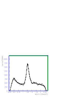
Figure 5: Fit to BES data using $1/D(s)$ derived from CCL phases.

3.1 Missing elements in the Roy solution

The Roy equation is in principle exact. How is it possible to modify the solution? In Nature, the Roy equation ‘knows’ about coupling of $\pi\pi$ to $KK$ and $\eta\eta$, as well as the $f_{0}(980)$, $f_{0}(1370)$ and $f_{0}(1500)$ resonances. If $\pi\pi$ phase shifts were known with errors of a small fraction of a degree, it would be possible to deduce these resonances and their couplings. However, that is not the present situation. In reality, there are subtle features in the processes $\pi\pi\to KK$ and $\eta\eta$ arising from meson exchanges and also from mixing between $\sigma$ and $f_{0}$.

Although the $\sigma$ pole appears remote from the $KK$ threshold, one must remember that the phase shift it produces reaches $90^{\circ}$ close to the position of $f_{0}(980)$, so multiple scattering is a maximum there. This includes terms of the form $\sigma\to\pi\pi$ (or $KK$) $\to f_{0}(980)$ leading to mixing. Anisovich, Anisovich and Sarantsev show [18] that this mixing obeys the Breit-Rabi equation, so $\sigma$ and $f_{0}(980)$ behave as a pair of coupled oscillators.

A recent paper with van Beveren, Rupp and Kleefeld [19] shows that the nonet of $\sigma$, $\kappa$, $a_{0}(980)$ and $f_{0}(980)$ may be generated by coupling of mesons to a $q\bar{q}$ loop. The $\sigma$ is generated by the $n\bar{n}$ loop and the $f_{0}(980)$ by the $s\bar{s}$ loop. Without mixing between $\sigma$ and $f_{0}$, one can only account for $<10\%$ of the observed magnitude of $f_{0}(980)\to\pi\pi$. Substantial mixing is required to produce the observed $\pi\pi$ width. Using their programme, I have tried varying the mixing angle and its $s$-dependence to examine perturbations of the $\pi\pi$ amplitude. Since the Schrödinger equation is solved, the amplitudes are fully analytic. In the mass range 700-1150 MeV, one sees subtle correlated changes in $\pi\pi$ phases and the inelasticity parameter $\eta$. These are not present in the calculation of CCL. The Roy equation is simply a dispersion relation between real and imaginary parts of the $\pi\pi\to\pi\pi$ amplitude. Its solution for the real part is only as good as the input for the imaginary part. They derive results for $f_{0}(980)$, $KK\to\pi\pi$ and $\eta\eta\to\pi\pi$ from my inelasticity parameters of Ref. [4]; but those are based upon simple Flatté parametrisations of $f_{0}$ and $\sigma$, without any dynamics due to mesons exchanges and mixing.

Calculations in Ref. [19] show that the $f_{0}$ pole is anchored to the $KK$ threshold. What happens as the mixing is varied is that an $f_{0}\to\pi\pi$ amplitude reaching down to the $\pi\pi$ threshold is generated. It is questionable exactly what its precise mass dependence will be. The best conjecture one can make at present is that it will contain the Adler zero of the full $\pi\pi$ amplitude, but otherwise behaves like a normal resonance. That is the conjecture adopted here. Calculations with the model of van Beveren et al show that the $\sigma$ pole can be affected by the mixing with $f_{0}(980)$ by up to 50 MeV. The reason for this is that the mixing alters the $s$-dependence of the $\pi\pi$ amplitude. The pole position is determined by the Cauchy-Riemann relations as one moves off the real $s$-axis. It lies far below the mass at which the $\pi\pi$ phase shift reaches $90^{\circ}$. Because of this long lever arm, even a small change of the slope of $\pi\pi$ phases v. mass can move the pole a surprisingly long way. This is why including an $f_{0}(980)$ contribution making up $7\%$ of the scattering length moves the pole position up to 467 MeV.

This degree of freedom is missing from the calculation of CCL. My conclusion is that it is legitimate to introduce into the fit small systematic perturbations in eqns. (4), (8) and (9) arising from inelasticities in $KK$ and $\eta\eta$ channels and also mixing between $\sigma$ and $f_{0}$. This secures agreement with BES data with only small changes in $\pi\pi$ phase shifts.

4 Refit of BES data

In the next fit, BES data are refitted together with $K_{e4}$ and Cern-Munich data as in the BES publication, but using the new equations of Section 2. The small $f_{0}(1370)$ and $f_{0}(1500)$ contributions are included in this fit (and the next). The scattering length $a_{0}$ and the effective range are fitted with the errors quoted by CCL. Parameters are shown in column (ii) of Table 1.

Resulting errors decrease compared with the BES publication because including $\sigma\to KK$ and $\eta\eta$ produces cusps at these thresholds and removes the requirement for the $f_{0}(980)$ contribution completely; the errors of $\pm 30$ MeV in real and imaginary parts of the pole position are taken from a range of fits to BES data using a variety of fitting functions going beyond those used here; they include systematic errors in data. The shift in the pole arises partly from the use of $j_{1}(s)$ of eqn. (6) but mostly from including $KK$ and $\eta\eta$ channels. There is a distinct improvement in the fit to BES data. This fit is used in making Fig. 1. It is a valuable feature of the BES data that the $f_{0}(980)$ contribution is negligible, giving an unimpeded view of the $\sigma$ pole.

The fit to phases is shown by the chain curve of Fig. 3 and the fit to BES data by the dashed curve of Fig. 4. The fitted value of $a_{0}$ falls to $0.189m_{\pi}^{-1}$, i.e. $6.2\sigma$ below the ChPT prediction. The question is whether to believe the ChPT prediction or the experimentally fitted scattering length. The ChPT prediction was made using the Roy equation which gives the low mass of CCL’s $\sigma$ pole. It is obvious that there will be a correlation between $a_{0}$ and the pole position: as the pole moves away from the $\pi\pi$ threshold, the scattering length will naturally decrease. If the scattering length is forced upwards, one finds an almost linear relation between the pole mass and the scattering length. To reach a value $a_{0}=0.215m_{\pi}^{-1}$ requires a pole mass of 472 MeV. The $\chi^{2}$ of the fit increases substantially, mostly because of the $K_{e4}$ and Cern-Munich data; in particular, the 382 MeV point of $K_{e4}$ data pulls the scattering length down. The BES data at low mass also favour a small scattering length, but are in a mass range where the available phase space is cutting off the signal.

It must be said that this fit is not using information from the Roy equation. It is made empirically to data above threshold. In the next step, the information from the Roy equation is incorporated as closely as possible.

4.1 A compromise solution

In order to constrain the fit to data as closely as possible to the Roy equation, a combined fit is made to the $T_{11}$ of CCL up to 1.15 GeV, and data from BES, $K_{e4}$ and Cern-Munich. Errors are assigned to CCL phases rising linearly with lab kinetic energy from zero at threshold to $3^{\circ}$ at 750 MeV. This gives maximum weight to results from the Roy equation near threshold, but allows flexibility in the effects of $f_{0}(980)$, and continuations of effects of $KK$ and $\eta\eta$ inelasticities into the mass range 600 to 1000 MeV. The pole moves to (472 - i 271) MeV and parameters are given in column (iii) of Table 1. The scattering length is $0.215m_{\pi}^{-1}$. The fit to BES data is shown by the full curve of Fig. 4; it is marginally poorer in terms of total $\chi^{2}$ but is obviously acceptable. However, the fit resists strongly any attempt to move the mass of the pole any lower and the scattering length correspondingly higher.

The fit to phases is shown by the dashed curve of Fig. 3. Up to 750 MeV, the difference between this fit and CCL phases is only $1.2^{\circ}$ at 470 MeV. This illustrates how difficult it is to deduce the $\sigma$ pole position from elastic data. The difference of $1.65^{\circ}$ at 865 MeV is well within errors of data.

Strictly speaking, the small perturbation to the $\sigma$ amplitude on the right-hand cut induces, via crossing, a small perturbation to the left-hand cut. However, the $\sigma$ contribution on the left-hand cut has a small isospin coefficient, and I have checked that in practice the perturbation is smaller than errors in the large contributions from $\rho$ and $f_{2}$ exchange.

What scattering length should be adopted? The lowest order prediction from Weinberg’s current algebra [20] is $0.16m_{\pi}^{-1}$. In second order ChPT it rises to $0.20m_{\pi}^{-1}$ and then $0.215m_{\pi}^{-1}$ at fourth order. The prediction of $(0.220\pm 0.005)m_{\pi}^{-1}$ at sixth order by Colangelo et al. [17] takes account of the unitarity branch cut at threshold; however, it does depend on using the Roy equations. It seems safe to constrain the scattering length to be at least $0.215m_{\pi}^{-1}$, so the conclusion is that fit (iii) is currently the best compromise. The change to the pole mass predicted by CCL is modest, but twice the error they quote.

The full and dashed curves of Fig. 4 are very similar. This is because they differ only in the scattering length $a_{0}$. An interesting result is that, for all three fits, the effective range does not change significantly from the CCL value. In lowest order ChPT, the effective range is proportional to

$$2a_{0}-5a_{2}=3m_{\pi}^{2}/4\pi F^{2}_{\pi},$$ (12)

as shown by Weinberg [19], so this relation is accurately consistent with all three fits. In this relation, $F_{\pi}$ is the pion decay constant.

5 Possible ambiguities in fitting BES data

Although the effect of systematic changes in inelasticity over the mass range from threshold to 1.15 GeV provides a natural resolution of the discrepancy between BES data and the CCL prediction, alternatives have been suggested. Two points have appeared in recent preprints. Firstly, Wu and Zou [21] remark that the width fitted to $b_{1}(1235)$ is 195 MeV compared with the value $142\pm 9$ MeV of the Particle Data Group [22]. This discrepancy was also reported by DM2 [2]. Wu and Zou suggest that the strong process $J/\Psi\to\rho\pi$, followed by $\rho\to\omega\pi$ may contribute. In the original BES work, the possibility $\rho(770)\to\omega\pi$ was tried and gave little improvement and, at maximum, a contribution of 2% (intensity) of the data. In any case, the effect lies close to the vertical and horizontal $b_{1}$ bands of Fig. 1(a), particularly the region where they cross near the bottom left-hand corner of the Dalitz plot. This is remote from the $\sigma$ band; changes to interferences between $\sigma$ and $b_{1}$, $\rho$ or $\rho^{\prime}$ have negligible effect on $\sigma$ parameters.

Secondly, Caprini [23] suggests that triangle graphs due to $b_{1}\to\omega\pi$, followed by $\pi\pi$ rescattering will introduce effects beyond the isobar model. Although this is true, it is known that such effects vary logarithmically over the Dalitz plot. There is no obvious reason why they should introduce a rapidly varying effect close to the right-hand edge of the Dalitz plot.

Thirdly, could there be some form of background in $J/\Psi\to\omega\sigma$? If such a background is included as a quadratic function of $s$, the discrepancy with CCL persists. The reason is that BES data determine the $\pi\pi$ S-wave amplitude accurately above the $f_{2}(1270)$ as well as below it and limit it to small values; this severely limits the form of any background to something close to the observed peak. In particular, a conventional form factor $\exp(-k^{2}R^{2}/6)$ at the vertex for $J/\Psi\to\omega\sigma$ (where $k$ is $\omega$ momentum in the $J/\Psi$ rest frame) gives no improvement, since it requires negative $R^{2}$. So a background does not provide a simple escape route.

A fourth possibility has been raised in discussions with CCL. This is that the form factor has a zero somewhere above 1 GeV. Extrapolating the full curve of Fig. 4, there might in principle be a zero in the mass range around 1.3 GeV. This would be obscured in the BES data on $J/\Psi\to\omega\pi\pi$ by the $f_{2}(1270)$. However, there are also data on $J/\Psi\to\omega K^{+}K^{-}$ where the $\sigma\to KK$ amplitude is clearly required [24]. The $f_{2}(1270)\to KK$ contribution in those data is sufficiently small that a zero in the $\sigma\to KK$ amplitude can be ruled out definitively up to $\sim 1.6$ GeV. At that mass, the required radius of interaction would be unreasonably large, $>0.8$ fm, and the $\sigma$ pole region would be seriously distorted by the form factor. Data on production of the $\kappa$ pole in $J/\Psi\to K^{*}(890)K\pi$ require an RMS radius $<0.38$ fm with 95% confidence [25].

6 Discussion and conclusions

There is a significant conflict in Fig. 4 between the $\sigma$ pole of CCL and BES data. In my view, the discrepancy needs explanation and the BES data should be taken at face value. The prescription adopted here in eqns. (4), (8) and (9) gives a natural improvement in fitting BES data without disturbing elastic phases up to 750 MeV by more than $1.2^{\circ}$ in fit (iii). This illustrates the ease with which the prediction of CCL may be modified to fit BES data.

The strength of the BES data is that a peak is clearly visible. There is no significant $f_{0}(980)$ signal. The BES data are therefore free of uncertainties about mixing between $\sigma$ and $f_{0}(980)$. The weakness of elastic scattering data is that there is no visible peak which can be checked, and there is a significant $f_{0}(980)$ amplitude which must be separated. The BES data provide a better view of the upper side of the $\sigma$ pole than elastic data, where the low mass tail of $f_{0}(980)$ is uncertain. The CCL calculation provides a better view of its lower side, where constraints from ChPT are valuable.

A more ambitious approach, beyond the scope of present work, would be a solution of coupled channel Roy equations for $\pi\pi$, $KK$ and $\eta\eta$ channels, including the dynamics driving $f_{0}(980)$ and $\sigma\to KK$ and $\eta\eta$. However, from experience with the model of van Beveren et al [19], it is likely that uncertainties are presently too large to give a definitive prediction of the dynamics of $f_{0}(980)$ and its delicate mixing with the $\sigma$.

I am grateful to Prof. H. Leutwyler for extensive discussions of the details of the calculation of Ref. [1]. I am also indebted to Profs. G. Rupp and E. van Beveren for use of their programme and Dr. F. Kleefeld for illuminating discussions.

References

- [1] Ablikim M et al 2004 Phys. Lett. B 598 149
- [2] Augustin J E et al 1989 Nucl. Phys. B 320 1
- [3] Aitala E M et al 2001 Phys. Rev. Lett. 86 770
- [4] Bugg D V Preprint hep-ex/0603023 and 2006 Eur. Phys. J C 47 45
- [5] Caprini I, Colangelo G and Leutwyler H 2006 Phys. Rev. Lett. 96 032001
- [6] Roy S M 1971 Phys. Lett. B 36 353
- [7] Link J M et al 2004 Phys. Lett. B 585 200
- [8] Pislak S et al 2001 Phys. Rev. Lett. 87 221801; Pislak S et al 2003 Phys. Rev. D 67 072004
- [9] Hyams B P et al 1973 Nucl. Phys. B 64 134
- [10] Bugg D V 2004 Eur. Phys. J C 37 433
- [11] Bugg D V, Sarantsev A V and Zou B S 1996 Nucl. Phys. B 471 59
- [12] Ablikim M et al 2005 Phys. Lett. B 607 243
- [13] Büttiker P, Descotes-Genon S and Moussallam B 2004 Eur. Phys. J C 33 409
- [14] Aloisio A et al 2002 Phys. Lett. B 537 21
- [15] Achasov N N and Ivanchenko V N 1989 Nucl. Phys. B 315 465
- [16] Ananthanarayan B, Colangelo G, Gasser J and Leutwyler H 2001 Phys. Rep. 353 207
- [17] Colangelo G, Gasser J and Leutwyler H 2001 Nucl. Phys. B 603 125
- [18] Anisovich A V, Anisovich V V and Sarantsev A V 1997 Zeit. Phys. A 359 173
- [19] van Beveren E, Rupp G, Bugg D V and Kleefeld F Preprint hep-ph/0606022 and 2006 Phys. Lett. B 641 265
- [20] Weinberg S 1966 Phys. Rev. Lett. D 17 616
- [21] Wu F Q and Zou B S Preprint hep-ph/0603224
- [22] Particle Data Group (PDG) 2004 Phys. Lett. B 592 1
- [23] Caprini I, Preprint hep-ph/0603250
- [24] Ablikim M et al 2004 Phys. Lett. B 603 138
- [25] Bugg D V 2006 Phys. Lett. B 632 471