ECT^∗-06-10

HD-THEP-06-16

hep-ph/0608082

Chiral Symmetry and Diffractive Neutral Pion
Photo- and Electroproduction

Carlo Ewerz ^a,1, Otto Nachtmann ^b,2

^a ECT ^∗, Strada delle Tabarelle 286, I-38050 Villazzano (Trento), Italy

^b Institut für Theoretische Physik, Universität Heidelberg
Philosophenweg 16, D-69120 Heidelberg, Germany

We show that diffractive production of a single neutral pion in photon-induced reactions at high energy is dynamically suppressed due to the approximate chiral symmetry of QCD. These reactions have been proposed as a test of the odderon exchange mechanism. We show that the odderon contribution to the amplitude for such reactions vanishes exactly in the chiral limit. This result is obtained in a nonperturbative framework and by using PCAC relations between the amplitudes for neutral pion and axial vector current production.

  ¹ email: Ewerz@ect.it
² email: O.Nachtmann@thphys.uni-heidelberg.de

1 Introduction

In this paper we study the diffractive production of a single neutral pion in the scattering of a real or virtual photon on a nucleon:

$$\gamma^{(*)}(q)+N(p)\,\longrightarrow\,\pi^{0}(q^{\prime})+X(p^{\prime})\,.$$ (1)

Here $N$ stands for a proton or a neutron, and $X$ denotes the rest of the hadronic final state which can consist of a single nucleon or of a group of hadrons. The four-momenta are indicated in brackets. The usual invariant variables are

$$s=(p+q)^{2}=(p^{\prime}+q^{\prime})^{2}\,,\quad\quad\quad t=(p-p^{\prime})=(q-q^{\prime})^{2}\,.$$ (2)

We always consider high energies, that is $s\gg m^{2}_{p}$. We assume that there is a large rapidity gap between $\pi^{0}$ and $X$ in (1). Since neutral pions have charge conjugation $C=+1$ these reactions are at high energy expected to occur due to the exchange of an odderon, the $C=-1$ partner of the well-established pomeron, see figure 1. (Note that throughout this paper we draw the incoming particles to the right.) For a review of high energy scattering in QCD see [1].

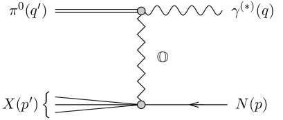
Figure 1: Diffractive production of a neutral pion in real or virtual photon-nucleon scattering due to exchange of an odderon ($\textstyle\mathbb{O}$).

The odderon was introduced many years ago [2, 3] and since then has been studied extensively from the theoretical point of view, for a review see [4]. Recently, particular progress has been made in understanding the odderon in the perturbative regime [5, 6]. From the experimental side the odderon has turned out to be an elusive object. There is some evidence for it in high energy proton-proton and antiproton-proton scattering [7] at a momentum transfer squared of $|t|\approx 1.0-1.5\,\mbox{GeV}^{2}$, see also [8] for a recent discussion. But otherwise conclusive evidence for the existence of the odderon is missing. In [9, 10, 11] it was suggested to look for the odderon in the reaction (1). Subsequently, the photoproduction of $\pi^{0}$ was investigated in detail in [12]. (For a discussion of the photoproduction of tensor and other pseudoscalar mesons see [13, 11].) The cross section at a c. m. energy of $\sqrt{s}=20$ GeV was predicted to be

$$\sigma(\gamma p\to\pi^{0}X)\approx 300\,{\rm nb}\,,$$ (3)

and only a weak dependence of this result on the energy $\sqrt{s}$ is expected. The uncertainties of the model of nonperturbative dynamics used in [12] imply a rather large uncertainty of about a factor $2$ in the prediction (3). However, corresponding experimental searches at HERA found no evidence for odderon-exchange reactions. The experimental search at $\sqrt{s}=200\,\mbox{GeV}$ [14] resulted in an upper limit of

$$\sigma(\gamma p\to\pi^{0}N^{*})<49\,{\rm nb}$$ (4)

at the 95 % confidence level, hence excluding the prediction (3) even if the large uncertainty inherent in the latter is taken into account. The non-observation of diffractive single pion production at HERA is especially striking since among all reactions in which hadrons are diffractively produced this reaction is the one with the largest kinematical phase space. Therefore there must be a dynamical mechanism which strongly suppresses the production rate.

In a short paper [15] possible causes for the failure of the calculations of [12] in comparison with experiment were discussed. One of them is a very low odderon intercept leading to a strong suppression of the cross section for the process (1) at high energies. A second possibility discussed in [15] is the failure of a factorisation hypothesis for field strength correlators that had been used in the nonperturbative model underlying the calculation of [12]. Another known source of suppression of odderon-induced reactions is the potentially small coupling of the odderon to the nucleon. A possible reason for the smallness of this coupling is a clustering of two constituent quarks of the nucleon into a small-size system of diquark type [16, 8]. However, the suppression due to that effect should only be relevant for reactions in which the proton stays intact, but should not lead to a sizable effect in reactions of type (1) in which the proton dissociates or is excited [17].

Finally, it was pointed out in [15] that a suppression of the cross section for diffractive single pion production can occur due to the particular properties of the wave function of the pion. These were not properly taken into account in the calculation leading to the prediction of [12]. It is in fact natural to expect that the special nature of the pion in the context of chiral symmetry can have considerable effects on the reaction (1).

In the present paper we give a detailed account of the latter argument. We shall show that the chiral symmetry of QCD leads to a vanishing amplitude for the reaction (1) when the limits of high energies and vanishing pion mass are taken. Our analysis is entirely based on nonperturbative techniques. In particular, we shall use the functional methods explained in detail in [18, 19] in connection with the dipole picture for photon-induced reactions.

Our paper is organised as follows. In section 2 we discuss $\pi^{0}$-production in a functional integral approach and use PCAC to relate this reaction to one involving the axial vector current. In section 3 we classify the contributions to the amplitude at high energies and identify the contributions which are leading at high energies. In section 4 we find the dependence of the latter on the light quark masses. In section 5 we study the renormalisation of the amplitudes under consideration and find that the dependence on the light quark masses remains unchanged. In section 6 we finally show that the leading terms at high energies in fact vanish in the chiral limit $m_{\pi}\rightarrow 0$, and we discuss this result. In appendix A we describe the functional methods used in section 3. In appendix B we outline how our results can be generalised to single diffractive pion production with a break-up of the nucleon.

2 The reactions $\gamma^{(*)}p\rightarrow\pi^{0}p$ and $\gamma^{(*)}p\rightarrow A^{3}p$

In this section we consider as an example for (1) neutral pion photo- and electroproduction on a proton

$$\gamma^{(*)}(q,\nu)+p(p,s)\,\longrightarrow\,\pi^{0}(q^{\prime})+p(p^{\prime},s^{\prime})\,.$$ (5)

Momenta and spin labels are indicated in brackets. We suppose

$$q^{2}=-Q^{2}\leq 0$$ (6)

and have for real pions

$$q^{\prime 2}=m^{2}_{\pi}\,.$$ (7)

Let $\phi^{a}(x)$ be a renormalised and correctly normalised interpolating field operator for the isotriplet of pions, $a=1,2,3$. We have then

$$\langle 0|\phi^{a}(x)|\pi^{b}(q^{\prime})\rangle=e^{-iq^{\prime}x}\delta_{ab}\,,$$ (8)

and the physical pion states are

$$|\pi^{0}(q^{\prime})\rangle = {}|\pi^{3}(q^{\prime})\rangle,$$

$$|\pi^{\pm}(q^{\prime})\rangle = {}\frac{1}{\sqrt{2}}\left(|\pi^{1}(q^{\prime})\rangle\pm i\,|\pi^{2}(q^{\prime})\rangle\right)\,.$$ (9)

The LSZ reduction formula [20] gives for the amplitude of (5)

$$(2\pi)^{4}\delta^{(4)}(p^{\prime}+q^{\prime}-p-q)\,{\cal M}^{\nu}_{s^{\prime}s}(\pi^{0};q^{\prime},p,q)$$ (10)

$$= {}-i\int d^{4}x^{\prime}\,d^{4}x\,e^{iq^{\prime}x^{\prime}}e^{-iqx}\left(\Box_{x^{\prime}}+m^{2}_{\pi}\right)\,\langle p(p^{\prime},s^{\prime})|{\rm T}^{*}\phi^{3}(x^{\prime})J^{\nu}(x)|p(p,s)\rangle\,.$$

Here $eJ^{\nu}(x)$ is the hadronic part of the electromagnetic current with $e$ the proton charge. With the quark field operator

$$\psi(x)=\left(\begin{array}[]{l}u(x)\\ d(x)\\ s(x)\\ c(x)\\ b(x)\\ t(x)\end{array}\right)$$ (11)

we have

$$J^{\nu}(x)=\bar{\psi}(x)\gamma^{\nu}\mathbf{Q}\psi(x)\,.$$ (12)

Here $\mathbf{Q}=$ diag$(Q_{u},\dots,Q_{t})$ is the quark charge matrix with $Q_{u}=2/3,~{}Q_{d}=-1/3$ etc. Our normalisation is such that the $T$-matrix element for (5) with a real photon of polarisation vector $\varepsilon^{\nu}$ is given by

$$\langle\pi^{0}(q^{\prime}),p(p^{\prime},s^{\prime})|{\cal T}|\gamma(q,\varepsilon),p(p,s)\rangle=e{\cal M}^{\nu}_{s^{\prime}s}(\pi^{0};q^{\prime},p,q)\,\varepsilon_{\nu}\,.$$ (13)

In (13) we have, of course, $q^{2}=0$ and $q^{\prime 2}=m^{2}_{\pi}$. Our conventions for kinematics, Dirac matrices etc. follow [21].

Starting from (10) we can extend the amplitude ${\cal M}^{\nu}_{s^{\prime}s}$ to off-shell pions, that is, we consider in the following ${\cal M}^{\nu}_{s^{\prime}s}(\pi^{0};q^{\prime},p,q)$ of (10) for

$$q^{\prime 2}\leq m^{2}_{\pi}\,,\quad\quad\quad q^{2}=-Q^{2}\leq 0\,.$$ (14)

The reaction which we consider along with (5) is

$$\gamma^{(*)}(q,\nu)+p(p,s)\,\longrightarrow\,A^{3}(q^{\prime},\mu)+p(p^{\prime},s^{\prime})\,,$$ (15)

that is, the production of an axial vector current instead of the $\pi^{0}$ meson. The isotriplet of axial vector currents is given by

$$A^{a}_{\mu}(x)=\bar{\psi}(x)\gamma_{\mu}\gamma_{5}\mathbf{T}_{a}\psi(x)\quad\quad(a=1,2,3)\,.$$ (16)

Here we denote by

$$\mathbf{T}_{a}=\left(\begin{array}[]{c|c}\frac{1}{2}\tau_{a}&0\\ \hline\cr 0&0\end{array}\right)$$ (17)

the flavour isospin matrices for the quarks, where the $\tau_{a}$ are the Pauli matrices. We define the amplitude for reaction (15) as

$$(2\pi)^{4}\delta^{(4)}(p^{\prime}+q^{\prime}-p-q)\,{\cal M}^{\mu\nu}_{s^{\prime}s}(A^{3};q^{\prime},p,q)$$ (18)

$$= {}\frac{i}{2\pi m_{p}}\int d^{4}x^{\prime}\,d^{4}x\,e^{iq^{\prime}x^{\prime}}e^{-iqx}\langle p(p^{\prime},s^{\prime})|\,{\rm T}^{*}A^{3\mu}(x^{\prime})J^{\nu}(x)|p(p,s)\rangle\,.$$

For (18) we consider again the kinematic region (14).

The well known PCAC relation (partially conserved axial vector current) relates the divergence of the currents (16) to a correctly normalised pion field operator,

$$\partial_{\lambda}A^{a\lambda}(x)=\frac{f_{\pi}m^{2}_{\pi}}{\sqrt{2}}\,\phi^{a}(x)\,,$$ (19)

see for example [22]. Here $f_{\pi}\cong 130\,\mbox{MeV}$ is the pion decay constant, see p. 496 of [23].

We insert now the PCAC relation (19) in (10) and get for $q^{\prime 2}<m^{2}_{\pi}$

$$(2\pi)^{4}\delta^{(4)}(p^{\prime}+q^{\prime}-p-q)\,{\cal M}^{\nu}_{s^{\prime}s}(\pi^{0};q^{\prime},p,q)$$

$$= {}-i\int d^{4}x^{\prime}\,d^{4}x~{}e^{iq^{\prime}x^{\prime}}e^{-iqx}\frac{\sqrt{2}}{f_{\pi}m^{2}_{\pi}}\,(-q^{\prime 2}+m^{2}_{\pi})\langle p(p^{\prime},s^{\prime})|\,{\rm T}^{*}\partial^{\prime}_{\mu}A^{3\mu}(x^{\prime})J^{\nu}(x)|p(p,s)\rangle\,.$$

An integration by parts and using the vanishing of the equal-time commutator

$$\left[A^{30}(x^{\prime}),J^{\nu}(x)\right]\,\delta(x^{\prime 0}-x^{0})=0$$ (21)

leads to

$${\cal M}^{\nu}_{s^{\prime}s}(\pi^{0};q^{\prime},p,q)=\frac{2\pi m_{p}\sqrt{2}}{f_{\pi}m^{2}_{\pi}}\,(-q^{\prime 2}+m^{2}_{\pi})\,iq^{\prime}_{\mu}{\cal M}^{\mu\nu}_{s^{\prime}s}(A^{3};q^{\prime},p,q)\,,$$ (22)

or, written differently,

$$iq^{\prime}_{\mu}{\cal M}^{\mu\nu}_{s^{\prime}s}(A^{3};q^{\prime},p,q)=-\frac{f_{\pi}m^{2}_{\pi}}{2\pi m_{p}\sqrt{2}}\,\frac{1}{q^{\prime 2}-m^{2}_{\pi}+i\epsilon}\,{\cal M}^{\nu}_{s^{\prime}s}(\pi^{0};q^{\prime},p,q)\,.$$ (23)

Let us as a side remark remind the reader at this point that taking the limit $q^{\prime 2}\rightarrow 0$ in (23) leads to a Goldberger-Treiman type relation [24]. Indeed, we can split the amplitude ${\cal M}^{\mu\nu}_{s^{\prime}s}(A^{3};q^{\prime},p,q)$ into the pion pole part (see figure 2) and the rest which has no pion pole.

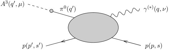
Figure 2: Pion-pole contribution to the amplitude ${\cal M}^{\mu\nu}_{s^{\prime}s}(A^{3};q^{\prime},p,q)$ in (18).

The pole term must be proportional to $q^{\prime\mu}$ and its residue is fixed by (22). We can take the pole term to be such that

$${\cal M}^{\mu\nu}_{s^{\prime}s}(A^{3};q^{\prime},p,q) = {}i\,\frac{f_{\pi}}{2\pi m_{p}\sqrt{2}}\,\frac{q^{\prime\mu}}{q^{\prime 2}-m^{2}_{\pi}+i\epsilon}\,{\cal M}^{\nu}_{s^{\prime}s}(\pi^{0};q^{\prime},p,q)$$ (24)

$${}+\left.{\cal M}^{\mu\nu}_{s^{\prime}s}(A^{3};q^{\prime},p,q)\right|_{\textup{non-pole}}\,.$$

Inserting this in (23) leads to

$$\frac{f_{\pi}}{2\pi m_{p}\sqrt{2}}\,\frac{(-m^{2}_{\pi})}{q^{\prime 2}-m^{2}_{\pi}+i\epsilon}\,{\cal M}^{\nu}_{s^{\prime}s}(\pi^{0};q^{\prime},p,q) = {}\frac{f_{\pi}}{2\pi m_{p}\sqrt{2}}\,\frac{(-q^{\prime 2})}{q^{\prime 2}-m^{2}_{\pi}+i\epsilon}\,{\cal M}^{\nu}_{s^{\prime}s}(\pi^{0};q^{\prime},p,q)$$ (25)

$${}+\left.iq^{\prime}_{\mu}{\cal M}^{\mu\nu}_{s^{\prime}s}(A^{3};q^{\prime},p,q)\right|_{\textup{non-pole}}\,.$$

Taking now the limit $q^{\prime 2}\rightarrow 0$ in (23) and (25) we get the Goldberger-Treiman type relation

$$\left.{\cal M}^{\nu}_{s^{\prime}s}(\pi^{0};q^{\prime},p,q)\right|_{q^{\prime 2}=0} = {}\frac{2\pi m_{p}\sqrt{2}}{f_{\pi}}\,iq^{\prime}_{\mu}\left.{\cal M}^{\mu\nu}_{s^{\prime}s}(A^{3};q^{\prime},p,q)\right|_{q^{\prime 2}=0}$$ (26)

$$= {}\frac{2\pi m_{p}\sqrt{2}}{f_{\pi}}\,iq^{\prime}_{\mu}\left.{\cal M}^{\mu\nu}_{s^{\prime}s}(A^{3};q^{\prime},p,q)\right|_{\textup{non-pole},\,q^{\prime 2}=0}.$$

Note that at $q^{\prime 2}=0$ the pion pole amplitude on the r.h.s. of (25) gives no contribution. The Goldberger-Treiman type relations are between the pion amplitude extrapolated to $q^{\prime 2}=0$ and the current amplitude $q^{\prime}_{\mu}{\cal M}^{\mu\nu}_{s^{\prime}s}(A^{3};q^{\prime},p,q)$ at $q^{\prime 2}=0$, where only the non-pole term contributes.

3 Classification of diagrams for $\gamma^{(*)}p\rightarrow A^{3}p$

In [18] we discussed real and virtual Compton scattering, $\gamma^{(*)}p\rightarrow\gamma^{(*)}p$, using functional methods. In particular, we gave a classification of contributions to the amplitude in terms of nonperturbative diagrams and identified the diagram classes which should be the leading ones at high energies; see section 2 of [18]. The general classification scheme into diagram classes (a) to (g) of figure 2 in [18] holds unchanged for reaction (15). All we have to do is to replace the electromagnetic current representing the final state photon in the Compton scattering case by the axial vector current. Most of the discussion of which nonperturbative diagrams are expected to be leading at high energies can be taken over from section 2.2 of [18]. There are diagrams with pure multi-gluon exchange in the $t$-channel as shown in figure 3a and 3b.

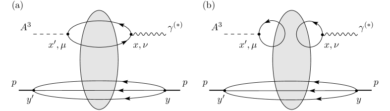
Figure 3: Diagrams which are expected to be the leading ones for reaction (15) at high energies.

In our case this exchange must have odderon quantum numbers, that is $C=-1$. The analogues of the diagrams (c) to (g) of figure 2 of [18] for our case correspond to quark exchange in the $t$-channel. As explained in section 2.2 of [18] such diagrams are expected to be suppressed for large $s$. Thus, the diagrams interesting for the odderon search are those shown in figure 3a and 3b. As explained in detail in [18] the full lines in figure 3 represent quark propagators in a fixed gluon potential. The shaded blobs indicate the functional integral over all gluon potentials with the measure given in (A.8) in appendix A. As in (13) of [18] we can now write

$${\cal M}^{\mu\nu}_{s^{\prime}s}(A^{3};q^{\prime},p,q)={\cal M}^{(a)\mu\nu}_{s^{\prime}s}(A^{3};q^{\prime},p,q)+\ldots+{\cal M}^{(g)\mu\nu}_{s^{\prime}s}(A^{3};q^{\prime},p,q)\,,$$ (27)

according to the decomposition of the amplitude in the diagram classes (a) to (g). The relevant terms for us here are

$${\cal M}^{(a)\mu\nu}_{s^{\prime}s}(A^{3};q^{\prime},p,q) = {}\left\langle U_{s^{\prime}s}(p^{\prime},p)\,A^{\mu\nu}(q^{\prime},q)\right\rangle_{G}\,,$$ (28)

$${\cal M}^{(b)\mu\nu}_{s^{\prime}s}(A^{3};q^{\prime},p,q) = {}\left\langle U_{s^{\prime}s}(p^{\prime},p)\right.\tilde{B}^{\mu}(q^{\prime})\left.B^{\nu}(q)\right\rangle_{G}\,.$$ (29)

More details are given in appendix A. The physical interpretation and analytic expressions of the terms in (28) and (29) are as follows. The scattering amplitude for the $\gamma^{(*)}$ converting to $A^{3\mu}$ in the fixed gluon potential $G$ (see the upper part of figure 3a) is given by

$$A^{\mu\nu}(q^{\prime},q)=\int d^{4}x^{\prime}\,d^{4}x\,e^{iq^{\prime}x^{\prime}}e^{-iqx}{\rm Tr}\left[\gamma^{\mu}\gamma_{5}\mathbf{T}_{3}\mathbf{S}_{F}(x^{\prime},x;G)\gamma^{\nu}\mathbf{Q}\,\mathbf{S}_{F}(x,x^{\prime};G)\right]\,.$$ (30)

Here

$$\mathbf{S}_{F}(x,x^{\prime};G)=\mathrm{diag}\left(S^{(u)}_{F}(x,x^{\prime};G),S^{(d)}_{F}(x,x^{\prime};G),\dots,S^{(t)}_{F}(x,x^{\prime};G)\right)$$ (31)

is the propagator matrix for the quarks moving in the fixed gluon potential $G$. The factor $B^{\nu}(q)$ in (29) represents the absorption of the photon in the fixed gluon potential (see figure 3b),

$$B^{\nu}(q)=\int d^{4}x\,e^{-iqx}i\,\mathrm{Tr}\left[\gamma^{\nu}\mathbf{Q}\,\mathbf{S}_{F}(x,x;G)\right]\,.$$ (32)

Similarly, the factor $\tilde{B}^{\mu}(q^{\prime})$ in (29) represents the creation of the axial vector current in the fixed gluon potential (see figure 3b),

$$\tilde{B}^{\mu}(q^{\prime})=\int d^{4}x^{\prime}\,e^{iq^{\prime}x^{\prime}}i\,\mathrm{Tr}\left[\gamma^{\mu}\gamma_{5}\mathbf{T}_{3}\mathbf{S}_{F}(x^{\prime},x^{\prime};G)\right]\,.$$ (33)

The factor $U_{s^{\prime}s}(p^{\prime},p)$ in (28) and (29) represents the scattering of the proton in the fixed gluon potential. It is given explicitly in (A.16) in appendix A, together with the expression for the functional integral $\langle\cdot\rangle_{G}$.

4 Divergence relations for axial vector amplitudes

In this section we study the divergences of the axial vector amplitudes in (28) and (29), that is $q^{\prime}_{\mu}A^{\mu\nu}(q^{\prime},q)$ and $q^{\prime}_{\mu}\tilde{B}^{\mu}(q^{\prime})$. For $A^{\mu\nu}(q^{\prime},q)$ we find from (30) with (A.6) and (A.7)

$$q^{\prime}_{\mu}A^{\mu\nu}(q^{\prime},q) = {}i\int d^{4}x^{\prime}\,d^{4}x\,e^{iq^{\prime}x^{\prime}}e^{-iqx}\frac{\partial}{\partial x^{\prime\mu}}\,\mathrm{Tr}\left[\gamma^{\mu}\gamma_{5}\mathbf{T}_{3}\mathbf{S}_{F}(x^{\prime},x;G)\gamma^{\nu}\mathbf{Q}\,\mathbf{S}_{F}(x,x^{\prime};G)\right]$$ (34)

$$= {}-\frac{1}{3}\int d^{4}x^{\prime}\,d^{4}x\,e^{iq^{\prime}x^{\prime}}e^{-iqx}$$

$${}\left\{2\,m^{(0)}_{u}\,\mathrm{Tr}\left[S^{(u)}_{F}(x,x^{\prime};G)\gamma_{5}S^{(u)}_{F}(x^{\prime},x;G)\gamma^{\nu}\right]\right.$$

$${}\left.{}+m^{(0)}_{d}\,\mathrm{Tr}\left[S^{(d)}_{F}(x,x^{\prime};G)\gamma_{5}S^{(d)}_{F}(x^{\prime},x;G)\gamma^{\nu}\right]\right\}\,.$$

We see explicitly here that $q^{\prime}_{\mu}A^{\mu\nu}(q^{\prime},q)$ contains one factor of the small $u$- and $d$-quark masses and inserting this in (28) we find the same for $q^{\prime}_{\mu}{\cal M}^{(a)\mu\nu}_{s^{\prime}s}(A^{3};q^{\prime},p,q)$. With (22) this implies that also ${\cal M}^{(a)\nu}_{s^{\prime}s}(\pi^{0};q^{\prime},p,q)$ contains one factor of $m_{u}$ or $m_{d}$. But as we shall see below this factor of the light quark masses is cancelled by the factor $m^{2}_{\pi}$ in the denominator in (22). The crucial observation which we will make in the present section is that $q^{\prime}_{\mu}A^{\mu\nu}(q^{\prime},q)$ is, in fact, proportional to the square of the light quark masses.

In order to trace the factors of the light quark masses in our amplitudes we will in the following make the dependence on $m_{q}^{(0)}$ explicit. We therefore indicate the dependence of the quark propagator on the quark mass by an additional argument,

$$S^{(q)}_{F}(x,x^{\prime};G)=S^{(q)}_{F}(x,x^{\prime};G,m^{(0)}_{q})\,.$$ (35)

We further introduce the free propagator for massless quarks,

$$S^{(q)}_{F}(x,y;0,0)=-\int\frac{d^{4}p}{(2\pi)^{4}}\,e^{-ip(x-y)}\,\frac{1}{\not\!p+i\epsilon}\,,$$ (36)

which satisfies (A.6) and (A.7) for $G=0$ and $m^{(0)}_{q}=0$. From the defining equations (A.6) and (A.7) for the full propagator we can easily derive the Lippmann-Schwinger relation

$$S^{(q)}_{F}(x,y;G,m^{(0)}_{q})=S^{(q)}_{F}(x,y;G,0)-\int d^{4}z\,S^{(q)}_{F}(x,z;G,0)\,m^{(0)}_{q}S^{(q)}_{F}(z,y;G,m^{(0)}_{q})\,.$$ (37)

In matrix notation where the space-time arguments and integrations are suppressed this reads

$$S^{(q)}_{F}(G,m^{(0)}_{q})=S^{(q)}_{F}(G,0)-S^{(q)}_{F}(G,0)\,m^{(0)}_{q}S^{(q)}_{F}(G,m^{(0)}_{q})\,.$$ (38)

Similarly, we find for the massless propagator the Lippmann-Schwinger relation

$$S^{(q)}_{F}(G,0)=S^{(q)}_{F}(0,0)-S^{(q)}_{F}(0,0)\,g^{(0)}\!\not\!G^{a}\frac{\lambda_{a}}{2}S^{(q)}_{F}(G,0)\,.$$ (39)

Here $g^{(0)}$ is the unrenormalised QCD coupling constant, and $\lambda_{a}$ are the Gell-Mann matrices. From (39) we get (still using matrix notation)

$$S^{(q)}_{F}(G,0) = {}\left[1+S^{(q)}_{F}(0,0)\,g^{(0)}\!\not\!G^{a}\frac{\lambda_{a}}{2}\right]^{-1}S^{(q)}_{F}(0,0)$$ (40)

$$= {}\sum^{\infty}_{n=0}\left(-S^{(q)}_{F}(0,0)\,g^{(0)}\!\not\!G^{a}\frac{\lambda_{a}}{2}\right)^{n}S^{(q)}_{F}(0,0)\,.$$

Since all terms on the r.h.s. of (40) have an odd number of $\gamma$ matrices we find immediately

$$S^{(q)}_{F}(x,x^{\prime};G,0)\gamma_{5}+\gamma_{5}S^{(q)}_{F}(x,x^{\prime};G,0)=0\,.$$ (41)

That is, the massless quark propagator in a fixed gluon potential anticommutes with $\gamma_{5}$.

Let us now consider for $q=u,d$ the trace part of the integrand in (34),

$$E^{\nu}(x,x^{\prime};G,m^{(0)}_{q})=\mathrm{Tr}\left[S^{(q)}_{F}(x,x^{\prime};G,m^{(0)}_{q})\gamma_{5}S^{(q)}_{F}(x^{\prime},x;G,m^{(0)}_{q})\gamma^{\nu}\right]\,.$$ (42)

Using (41) together with the cyclicity of the trace we find immediately for $m^{(0)}_{q}=0$

$$E^{\nu}(x,x^{\prime};G,0)=0\,.$$ (43)

With this and (38) we get for $E^{\nu}$ of (42)

$$E^{\nu}(x,x^{\prime};G,m^{(0)}_{q})=m^{(0)}_{q}E^{\prime\nu}(x,x^{\prime};G,0)+{\cal O}\left((m^{(0)}_{q})^{2}\right)\,,$$ (44)

where

$$m^{(0)}_{q}E^{\prime\nu}(x,x^{\prime};G,0)$$

$${}=-\int d^{4}z\,\mathrm{Tr}\left[S^{(q)}_{F}(x,z;G,0)\,m^{(0)}_{q}S^{(q)}_{F}(z,x^{\prime};G,0)\gamma_{5}S^{(q)}_{F}(x^{\prime},x;G,0)\gamma^{\nu}\right.$$

$${}\left.\hskip 71.13188pt{}+S^{(q)}_{F}(x,x^{\prime};G,0)\gamma_{5}S^{(q)}_{F}(x^{\prime},z;G,0)\,m^{(0)}_{q}S^{(q)}_{F}(z,x;G,0)\gamma^{\nu}\right]\,.$$

Note that only the massless propagator occurs in this expression. The presence of the massless propagator might potentially lead to infrared divergences when we consider the renormalisation of our amplitudes in the next section. But since we need to consider only the leading term in the light quark mass in the expansion (44) we can easily avoid this potential problem. Namely, we can replace the massless propagator in (4) by the massive propagator. The resulting expansion

$$E^{\nu}(x,x^{\prime};G,m^{(0)}_{q})=m^{(0)}_{q}E^{\prime\nu}(x,x^{\prime};G,m^{(0)}_{q})+{\cal O}\left((m^{(0)}_{q})^{2}\right)$$ (46)

with

$$m^{(0)}_{q}E^{\prime\nu}(x,x^{\prime};G,m^{(0)}_{q})$$

$${}=-\int d^{4}z\,\mathrm{Tr}\left[S^{(q)}_{F}(x,z;G,m^{(0)}_{q})\,m^{(0)}_{q}S^{(q)}_{F}(z,x^{\prime};G,m^{(0)}_{q})\gamma_{5}S^{(q)}_{F}(x^{\prime},x;G,m^{(0)}_{q})\gamma^{\nu}\right.$$

$${}\left.\hskip 56.9055pt{}+S^{(q)}_{F}(x,x^{\prime};G,m^{(0)}_{q})\gamma_{5}S^{(q)}_{F}(x^{\prime},z;G,m^{(0)}_{q})\,m^{(0)}_{q}S^{(q)}_{F}(z,x;G,m^{(0)}_{q})\gamma^{\nu}\right]$$

differs from (44) only in terms of higher order in the quark mass due to (38). The diagrams representing $E^{\prime\nu}$ are shown in figure 4.

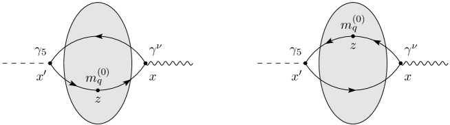
Figure 4: Diagrammatic representation of $m_{q}^{(0)}E^{\prime\nu}(x,x^{\prime};G,m^{(0)}_{q})$ (4) as the sum of two quark loops in a given gluon potential.

They correspond to a loop with a photon vertex, a pseudoscalar vertex, and a scalar vertex representing the quark mass insertion. Inserting (46) and (4) in (34) we see that $q^{\prime}_{\mu}A^{\mu\nu}(q^{\prime},q)$ is proportional to $(m^{(0)}_{q})^{2}$,

$$q^{\prime}_{\mu}A^{\mu\nu}(q^{\prime},q) = {}-\frac{1}{3}\int d^{4}x^{\prime}\,d^{4}x\,e^{iq^{\prime}x^{\prime}}e^{-iqx}$$ (48)

$${}\hskip 28.45274pt\left[\,2(m^{(0)}_{u})^{2}E^{\prime\nu}(x,x^{\prime};G,m^{(0)}_{u})+(m^{(0)}_{d})^{2}E^{\prime\nu}(x,x^{\prime};G,m^{(0)}_{d})\right]$$

$${}+{\cal O}\left((m^{(0)}_{u})^{3},(m^{(0)}_{d})^{3}\right)\,.$$

In a similar way we can discuss the divergence of the amplitude $\tilde{B}^{\mu}(q^{\prime})$ (33). We find

$$q^{\prime}_{\mu}\tilde{B}^{\mu}(q^{\prime})\!\! = {}\!\!iq^{\prime}_{\mu}\frac{1}{2}\int d^{4}x^{\prime}\,e^{iq^{\prime}x^{\prime}}\mathrm{Tr}\left[\gamma^{\mu}\gamma_{5}S^{(u)}_{F}(x^{\prime},x^{\prime};G,m^{(0)}_{u})-\gamma^{\mu}\gamma_{5}S^{(d)}_{F}(x^{\prime},x^{\prime};G,m^{(0)}_{d})\right]$$ (49)

$$= {}\!\!-i\int d^{4}x^{\prime}\,e^{iq^{\prime}x^{\prime}}\left\{m^{(0)}_{u}\mathrm{Tr}\left[\gamma_{5}S^{(u)}_{F}(x^{\prime},x^{\prime};G,m^{(0)}_{u})\right]\right.$$

$${}\hskip 73.97733pt\left.{}-m^{(0)}_{d}\mathrm{Tr}\left[\gamma_{5}S^{(d)}_{F}(x^{\prime},x^{\prime};G,m^{(0)}_{d})\right]\right\}\,.$$

Note that in the isospin symmetry limit, that is for $m^{(0)}_{u}=m^{(0)}_{d}$, we have $q^{\prime}_{\mu}\tilde{B}^{\mu}(q^{\prime})=0$. But in reality the light quark masses are small but quite different, see [25] and below. For the trace part of the integrand in (49) we easily find with (38)-(41) for $q=u,d$

$$F(x^{\prime};G,m^{(0)}_{q}) = {}\mathrm{Tr}\left[\gamma_{5}S^{(q)}_{F}(x^{\prime},x^{\prime};G,m^{(0)}_{q})\right]$$ (50)

$$= {}m^{(0)}_{q}F^{\prime}(x^{\prime};G,0)+{\cal O}\left((m^{(0)}_{q})^{2}\right)\,,$$

and

$$m^{(0)}_{q}F^{\prime}(x^{\prime};G,0)=-\int d^{4}z\,\mathrm{Tr}\left[\gamma_{5}S^{(q)}_{F}(x^{\prime},z;G,0)\,m^{(0)}_{q}S^{(q)}_{F}(z,x^{\prime};G,0)\right]\,.$$ (51)

Again we find it convenient to replace the massless propagator in this expression by the propagator for massive quarks as we did from (4) to (4). Hence we write

$$F(x^{\prime};G,m^{(0)}_{q})=m^{(0)}_{q}F^{\prime}(x^{\prime};G,m^{(0)}_{q})+{\cal O}\left((m^{(0)}_{q})^{2}\right)$$ (52)

with

$$m^{(0)}_{q}F^{\prime}(x^{\prime};G,m^{(0)}_{q})=-\int d^{4}z\,\mathrm{Tr}\left[\gamma_{5}S^{(q)}_{F}(x^{\prime},z;G,m^{(0)}_{q})\,m^{(0)}_{q}S^{(q)}_{F}(z,x^{\prime};G,m^{(0)}_{q})\right]\,,$$ (53)

which differs from (51) only by terms of higher order in $m_{q}^{(0)}$. The diagram corresponding to (53) is shown in figure 5.

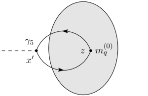
Figure 5: Diagrammatic representation of $m_{q}^{(0)}F^{\prime}(x^{\prime};G,m^{(0)}_{q})$ (53) as a quark loop in a given gluon potential.

We have a quark loop with one pseudoscalar and one scalar vertex, and the latter is again given by a quark mass insertion. Inserting (52) and (53) in (49) we see that also $q^{\prime}_{\mu}\tilde{B}^{\mu}(q^{\prime})$ is proportional to the square of the light quark masses,

$$q^{\prime}_{\mu}\tilde{B}^{\mu}(q^{\prime}) = {}-i\int d^{4}x^{\prime}\,e^{iq^{\prime}x^{\prime}}\left[(m^{(0)}_{u})^{2}F^{\prime}(x^{\prime};G,m^{(0)}_{u})-(m^{(0)}_{d})^{2}F^{\prime}(x^{\prime};G,m^{(0)}_{d})\right]$$ (54)

$${}{}+{\cal O}\left((m^{(0)}_{u})^{3},(m^{(0)}_{d})^{3}\right)\,.$$

As a final point in this section we discuss the question of possible anomalous contributions [26, 27, 28, 29] in the divergence relations (34) and (49). We are dealing here with the divergence of axial vector currents in an external vector (here: gluon) field and this is precisely the case studied explicitly in [27]. The electromagnetic part of the anomaly is not relevant for us here since in our reactions (5) and (15) only one photon is involved. The gluon anomaly on the other hand is relevant for us. The divergence of the axial vector current for one quark flavour reads

$$\partial_{\mu}\bar{q}(x)\gamma^{\mu}\gamma_{5}q(x)=2im^{(0)}_{q}\bar{q}(x)\gamma_{5}q(x)+\frac{(g^{(0)})^{2}}{32\pi^{2}}\,\epsilon_{\mu\nu\rho\sigma}G^{\mu\nu}(x)G^{\rho\sigma}(x)\,,$$ (55)

where we use the convention $\epsilon_{0123}=1$. The anomalous gluonic part of the divergence of the axial vector current in (55) is, however, independent of the quark mass. Thus the anomalous gluonic pieces cancel in the divergence of the axial vector current $A^{3}_{\mu}$ of (16) since

$$A^{3}_{\mu}(x)=\frac{1}{2}\bar{u}(x)\gamma_{\mu}\gamma_{5}u(x)-\frac{1}{2}\bar{d}(x)\gamma_{\mu}\gamma_{5}d(x)\,.$$ (56)

5 Renormalisation

So far our formulae are expressed in terms of bare quantities. In the present section we want to consider the renormalisation procedure for the amplitudes obtained above.

We use (48) to obtain from (28)

$$q^{\prime}_{\mu}{\cal M}^{(a)\mu\nu}_{s^{\prime}s}(A^{3};q^{\prime},p,q)=\langle U_{s^{\prime}s}(p^{\prime},p)q^{\prime}_{\mu}A^{\mu\nu}(q^{\prime},q)\rangle_{G}$$

$$= {}-\frac{1}{3}\int d^{4}x^{\prime}\,d^{4}x\,e^{iq^{\prime}x^{\prime}}e^{-iqx}$$

$${}\left\langle U_{s^{\prime}s}(p^{\prime},p)\left[\,2(m^{(0)}_{u})^{2}E^{\prime\nu}(x,x^{\prime};G,m^{(0)}_{u})+(m^{(0)}_{d})^{2}E^{\prime\nu}(x,x^{\prime};G,m^{(0)}_{d})\right]\right\rangle_{G}\,.$$

Here and in the following terms of cubic or higher order in the light quark masses are neglected. Using the methods described in appendix A we can show that this expression can also be obtained as the contribution of diagram class (a) contained in the following correlation function,

$$(2\pi)^{4}\delta^{(4)}(p^{\prime}+q^{\prime}-p-q)\,q^{\prime}_{\mu}{\cal M}^{(a)\mu\nu}_{s^{\prime}s}(A^{3};q^{\prime},p,q)$$

$$= {}\!\!-\frac{1}{2\pi m_{p}}\int d^{4}x^{\prime}\,d^{4}x\,d^{4}z\,e^{iq^{\prime}x^{\prime}}e^{-iqx}$$

$${}\hskip 14.22636pt{}\langle p(p^{\prime},s^{\prime})|\,\mathrm{T}^{*}\left[\left(m^{(0)}_{u}\bar{u}(x^{\prime})\gamma_{5}u(x^{\prime})\right)\left(m^{(0)}_{u}\bar{u}(z)u(z)\right)\right.$$

$${}\hskip 71.13188pt{}\left.\left.{}-\left(m^{(0)}_{d}\bar{d}(x^{\prime})\gamma_{5}d(x^{\prime})\right)\left(m^{(0)}_{d}\bar{d}(z)d(z)\right)\right]J^{\nu}(x)\,|p(p,s\rangle\,\right|_{(a)}\,,$$

see also figure 6 below. The subscript $(a)$ in this expression indicates that only the diagrams of type (a) of the correlation function in the integrand are taken into account.

We can obtain the divergence of ${\cal M}^{(b)\mu\nu}$ in a completely analogous way. We get from (29), (49), (52) and (54)

$$q^{\prime}_{\mu}{\cal M}^{(b)\mu\nu}_{s^{\prime}s}(A^{3};q^{\prime},p,q)=\langle U_{s^{\prime}s}(p^{\prime},p)q^{\prime}_{\mu}\tilde{B}^{\mu}(q^{\prime})B^{\nu}(q)\rangle_{G}$$

$$= {}\!\!-i\int d^{4}x^{\prime}\,e^{iq^{\prime}x^{\prime}}$$

$${}\left\langle U_{s^{\prime}s}(p^{\prime},p)\left[(m^{(0)}_{u})^{2}F^{\prime}(x^{\prime};G,m^{(0)}_{u})-(m^{(0)}_{d})^{2}F^{\prime}(x^{\prime};G,m^{(0)}_{d})\right]B^{\nu}(q)\right\rangle_{G}\,.$$

We can then relate this expression to the correlation function on the r.h.s. of (5) involving pseudoscalar, scalar and vector currents, but now taking into account only the diagrams of type (b).

It is well known (see for instance [30]) that the quark mass and the scalar and pseudoscalar currents have the same renormalisation constant $Z_{mq}$. We have for the masses

$$m^{R}_{q}=m^{(0)}_{q}Z^{-1}_{mq}\quad\quad\quad(q=u,d)\,,$$ (60)

where for definiteness we choose $m^{R}_{q}$ to be the renormalised quark masses in the $\overline{MS}$ scheme at renormalisation point $\mu=2\,\mbox{GeV}$, see [23]. The corresponding renormalised scalar and pseudoscalar currents are

$$(\bar{q}(x)q(x))^{R} = {}Z_{mq}\,\bar{q}(x)q(x),$$

$$(\bar{q}(x)\gamma_{5}q(x))^{R} = {}Z_{mq}\,\bar{q}(x)\gamma_{5}q(x)\quad\quad\quad(q=u,d)\,.$$ (61)

We have thus

$$m^{R}_{q}\left(\bar{q}(x)q(x)\right)^{R} = {}m^{(0)}_{q}\bar{q}(x)q(x)\,,$$

$$m^{R}_{q}\left(\bar{q}(x)\gamma_{5}q(x)\right)^{R} = {}m^{(0)}_{q}\bar{q}(x)\gamma_{5}q(x)\,.$$ (62)

We insert (5) in (5) and add the corresponding contribution for the divergence of the amplitude ${\cal M}^{(b)}$ to get

$$(2\pi)^{4}\delta^{(4)}(p^{\prime}+q^{\prime}-p-q)\,q^{\prime}_{\mu}{\cal M}^{(a+b)\mu\nu}_{s^{\prime}s}(A^{3};q^{\prime},p,q)$$

$$= {}-\frac{1}{2\pi m_{p}}\int d^{4}x^{\prime}\,d^{4}x\,d^{4}z\,e^{iq^{\prime}x^{\prime}}e^{-iqx}$$

$${}\left\{\left.{}(m^{R}_{u})^{2}\,\langle p(p^{\prime},s^{\prime})|\,\mathrm{T}^{*}(\bar{u}(x^{\prime})\gamma_{5}u(x^{\prime}))^{R}(\bar{u}(z)u(z))^{R}J^{\nu}(x)|p(p,s)\rangle\right|_{(a+b)}\right.$$

$${}\left.\left.{}-(m^{R}_{d})^{2}\,\langle p(p^{\prime},s^{\prime})|\,\mathrm{T}^{*}(\bar{d}(x^{\prime})\gamma_{5}d(x^{\prime}))^{R}(\bar{d}(z)d(z))^{R}J^{\nu}(x)|p(p,s)\rangle\right|_{(a+b)}\right\}\,.$$

Here we have used that in QCD the vector current $J^{\nu}(x)$ does not get renormalised. We now define ${\cal C}_{s^{\prime}s}^{(q)\nu}$ by

$${}(2\pi)^{4}\delta^{(4)}(p^{\prime}+q^{\prime}-p-q)\,{\cal C}^{(q)\nu}_{s^{\prime}s}(q^{\prime},p,q)$$ (64)

$$= {}-\frac{1}{2\pi m_{p}}\int d^{4}x^{\prime}\,d^{4}x\,d^{4}z\,e^{iq^{\prime}x^{\prime}}e^{-iqx}$$

$${}\left.\langle p(p^{\prime},s^{\prime})|\,\mathrm{T}^{*}(\bar{q}(x^{\prime})\gamma_{5}q(x^{\prime}))^{R}(\bar{q}(z)q(z))^{R}J^{\nu}(x)|p(p,s)\rangle\right|_{(a+b)}\,.$$

The diagrams for the integrand in (64) are shown in figure 6. Note that even for massless quarks we have ${\cal C}_{s^{\prime}s}^{(u)\nu}\neq{\cal C}_{s^{\prime}s}^{(d)\nu}$, because $u$ and $d$ quarks contribute differently in the current $J^{\nu}$. Since ${\cal C}^{(q)\nu}$ in (64) involves only renormalised quantities it should be finite. With (64) we obtain from (5)

$$q^{\prime}_{\mu}{\cal M}^{(a+b)\mu\nu}_{s^{\prime}s}(A^{3};q^{\prime},p,q)=(m^{R}_{u})^{2}\,{\cal C}^{(u)\nu}_{s^{\prime}s}(q^{\prime},p,q)-(m^{R}_{d})^{2}\,{\cal C}^{(d)\nu}_{s^{\prime}s}(q^{\prime},p,q)\,.$$ (65)

In (5) and (65) we have again neglected terms of cubic or higher order in the light quark masses.

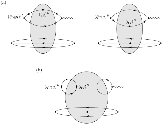
Figure 6: The diagrams of type (a) and (b) represent the correlation function ${\cal C}^{(q)\nu}_{s^{\prime}s}$ of (64).

With (65) we have shown that the divergence amplitude $q^{\prime}_{\mu}{\cal M}^{(a+b)\mu\nu}_{s^{\prime}s}(A^{3};q^{\prime},p,q)$ is indeed proportional to the square of the renormalised light quark masses.

6 Results and conclusions

It is well known that the light quark masses are directly related to $m^{2}_{\pi}$. Indeed one finds in the chiral limit (see (8.1) of [25]) for the average of the quark masses

$$\hat{m}\equiv\frac{1}{2}(m^{R}_{u}+m^{R}_{d})=\frac{1}{2B}\,m^{2}_{\pi}\,.$$ (66)

Here

$$B=-\frac{2}{f^{2}_{\pi}}\langle 0|\left(\bar{u}(x)u(x)\right)^{R}|0\rangle$$ (67)

is a hadronic constant which stays finite in the chiral limit $m^{R}_{u,d}\rightarrow 0$.

Experimentally the light quark masses still are not too well known, see [23]. In the following we take our estimates of ‘central’ values extracted from [23] and assume these masses to be $m_{u}^{R}\cong 3\,\mbox{MeV}$ and $m_{d}^{R}\cong 7\,\mbox{MeV}$ at a renormalisation scale of $2\,\mbox{GeV}$. This gives $\hat{m}\cong 5\,\mbox{MeV}$, and with $m_{\pi}=135\,\mbox{MeV}$ we get $B\cong 1820\,\mbox{MeV}$. The ratios of the light quark masses and the mean are then

$$r_{u}=\frac{m^{R}_{u}}{\hat{m}}\cong 0.6\,,\quad\quad\quad r_{d}=\frac{m^{R}_{d}}{\hat{m}}\cong 1.4\,.$$ (68)

Now we go back to (22) and discuss the quark mass, respectively $m^{2}_{\pi}$, dependence of ${\cal M}^{\nu}_{s^{\prime}s}(\pi^{0};q^{\prime},p,q)$ in the chiral limit $m^{R}_{u,d}\rightarrow 0$. For high energies we consider only the odderon-exchange diagrams (a) and (b) of figure 3 for the reasons given in section 3. We have then for the amplitudes corresponding to the sum of those diagrams

$${\cal M}^{(a+b)\nu}_{s^{\prime}s}(\pi^{0};q^{\prime},p,q)\equiv\frac{2\pi m_{p}\sqrt{2}}{f_{\pi}m^{2}_{\pi}}\,(-q^{\prime 2}+m^{2}_{\pi})\,iq^{\prime}_{\mu}{\cal M}^{(a+b)\mu\nu}_{s^{\prime}s}(A^{3};q^{\prime},p,q)$$ (69)

and obtain from (65) with (66), (68)

$${\cal M}^{(a+b)\nu}_{s^{\prime}s}(\pi^{0};q^{\prime},p,q) = {}m^{2}_{\pi}\,\frac{\pi m_{p}}{f_{\pi}B^{2}\sqrt{2}}\left[-r^{2}_{u}\,i(q^{\prime 2}-m^{2}_{\pi})\,{\cal C}^{(u)\nu}_{s^{\prime}s}(q^{\prime},p,q)\right.$$ (70)

$${}\hskip 62.59596pt\left.{}+r^{2}_{d}\,i(q^{\prime 2}-m^{2}_{\pi})\,{\cal C}^{(d)\nu}_{s^{\prime}s}(q^{\prime},p,q)\right]\,.$$

The correlation functions ${\cal C}^{(u)\nu}$ and ${\cal C}^{(d)\nu}$ occurring in (70) are properly renormalised. It is clear from their definition in (64) (see also figure 6) that they will have pion poles which are just cancelled by the explicit factors $(q^{\prime 2}-m^{2}_{\pi})$ in (70). Otherwise these functions should be finite in the chiral limit. Also $m_{p}$, $f_{\pi}$ and $B$ are known to approach finite values in the chiral limit, see for example [25]. Thus, due to the explicit factor $m^{2}_{\pi}$ in (70) the odderon-exchange amplitude for the reaction $\gamma^{(*)}p\to\pi^{0}p$ vanishes in the chiral limit $m^{2}_{\pi}\rightarrow 0$. This is the main result of the present paper.

In the case of approximate chiral symmetry, as realised in Nature, we do not expect the odderon-exchange amplitude for the reaction $\gamma^{(*)}p\to\pi^{0}p$ to vanish exactly. But from the above result we should expect that the approximate chiral symmetry leads to a strong dynamical suppression of this amplitude. It is difficult to assess the numerical effect of this suppression, a rough estimate has been given in [15]. It indicates that the effect of approximate chiral symmetry can modify the prediction (3) of [12] such as to reconcile it with the experimental upper bound (4) on the diffractive photoproduction of neutral pions.

Our result (70) holds for all photon virtualities $Q^{2}$ and momentum transfers $\sqrt{-t}$. In particular, it should also extend into the perturbative region of large $Q^{2}$ or large $\sqrt{-t}$. In this context it is worth pointing out that the result matches nicely the perturbative result of [31] where the diffractive reaction $\gamma^{(*)}p\to\eta_{c}\,p$ was considered at high energies. In that reaction perturbation theory can be applied because of the large scale given by the charm quark mass. In leading order in perturbation theory only diagrams of type (a) contribute to the $\gamma^{(*)}\to\eta_{c}$ impact factor. In [31] this impact factor was computed for an arbitrary number of gluons exchanged in the $t$-channel. It was found that for any number of exchanged gluons the impact factor, and hence the amplitude for that reaction, is linear in the quark mass. That agrees with the result that we find here based on general nonperturbative calculations, and the mechanism leading to that result is in fact the perturbative realisation of the one that we have described here in section 4.

Let us point out that we can easily extend our result to the general reaction (1) with nucleon dissociation. As an example we discuss in appendix B the reactions

$$\gamma^{(*)}(q,\nu)+p(p,s)\rightarrow\pi^{0}(q^{\prime})+n(p^{\prime}_{1},s^{\prime})+\pi^{+}(p^{\prime}_{2})$$ (71)

and

$$\gamma^{(*)}(q,\nu)+p(p,s)\rightarrow A^{3}(q^{\prime},\mu)+n(p^{\prime}_{1},s^{\prime})+\pi^{+}(p^{\prime}_{2})\,.$$ (72)

With the same techniques as above we find that taking the divergence of the odderon-exchange diagrams for (72) (see figure 7) gives an explicit factor $m^{2}_{\pi}$ in the amplitude for (71). That is, the odderon-exchange contribution to the reaction (71) vanishes in the chiral limit.

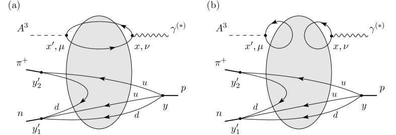
Figure 7: Odderon exchange diagrams for $\gamma^{*}p\rightarrow A^{3}n\pi^{+}$, reaction (72).

Finally, our findings can also be generalised to reactions of two real or virtual photons which will be relevant at the LHC and at a future ILC. Namely, it is straightforward to apply the same techniques to the diffractive reaction $\gamma^{(*)}+\gamma^{(*)}\to\pi^{0}+X$ at high energy. Again we find that the amplitude for the odderon-exchange contribution to this process is proportional to $m_{\pi}^{2}$ and vanishes in the chiral limit. In the diffractive reaction $\gamma^{(*)}+\gamma^{(*)}\to\pi^{0}+\pi^{0}$ the odderon-exchange contribution is even suppressed by a factor $m_{\pi}^{4}$ in the amplitude. We therefore expect the cross sections for these processes to be very small at high energies, independently of the odderon intercept.

To summarise, we have studied the diffractive photo- and electroproduction of a neutral pion on a nucleon, $\gamma^{(*)}+N\to\pi^{0}+X$ (reaction (1)). We have shown that the diagrams with multi-gluon exchange in the $t$-channel, that is the odderon exchange diagrams, vanish in the chiral limit. In the real world with approximate chiral symmetry these diagrams are dynamically suppressed by a factor $m_{\pi}^{2}$, and hence the cross section by a factor $m_{\pi}^{4}$. At high energies the other types of diagrams for reaction (1) (see figure 2 of [18]) are expected to be suppressed by inverse powers of the c. m. energy. Thus we have as a firm prediction of QCD that the cross sections for the reactions (1) should be very small at high energies compared to cross sections for reactions in which pomeron exchange is allowed like for instance $\gamma^{(*)}+N\to\rho^{0}+X$.

Appendix A Functional methods

Here we give a short outline of the functional method introduced in [18] which is used to derive (28) and (29). We start from (2) and use the LSZ reduction formula [20] to represent the amplitude as an integral over a Green’s function. The latter is then represented as a functional integral and the quark degrees of freedom are integrated out, giving rise to nonperturbative quark propagators in a given gluon potential. This leads to a number of nonperturbative diagrams distinguished by the topology of the quark-line skeleton.

In detail, let $\psi_{p}(x)$ be a suitable interpolating field operator for the proton. We can take $\psi_{p}$ to contain three quark fields,

$$\psi_{p}(x)=\Gamma_{\alpha\beta\gamma}u_{\alpha}(x)u_{\beta}(x)d_{\gamma}(x)\,,$$ (A.1)

and accordingly

$$\bar{\psi}_{p}(x)=\bar{\Gamma}_{\alpha\beta\gamma}\bar{d}_{\gamma}(x)\bar{u}_{\beta}(x)\bar{u}_{\alpha}(x)\,,$$ (A.2)

where $\Gamma_{\alpha\beta\gamma}$ and $\bar{\Gamma}_{\alpha\beta\gamma}$ are coefficient matrices and $\alpha,\beta,\gamma$ summarise Dirac and colour indices. Explicit constructions of field operators $\psi_{p}(x)$ of the type (A.1) can be found in [32, 33, 34]. Let $Z_{p}$ be the proton’s wave function renormalisation constant defined by

$$\left\langle 0|\psi_{p}(x)|p(p,s)\right\rangle=\sqrt{Z_{p}}\,e^{-ipx}u_{s}(p)\,.$$ (A.3)

As explained above, the amplitude (18) can be represented in terms of a functional integral

$${\cal M}^{\mu\nu}_{s^{\prime}s}(A^{3};q^{\prime},p,q)=-\frac{i}{2\pi m_{p}Z_{p}}\int d^{4}x^{\prime}\,d^{4}x\,d^{4}y\,e^{iq^{\prime}x^{\prime}}e^{-iqx}e^{-ipy}$$ (A.4)

$${}\left\{\bar{u}_{s^{\prime}}(p^{\prime})(-i\!\stackrel{{\scriptstyle\rightarrow}}{{\!\not\!\partial}}_{y^{\prime}}+m_{p})\frac{1}{{\cal Z}}\int{\cal D}(G,q,\bar{q})\,\bar{\psi}(x^{\prime})\gamma^{\mu}\gamma_{5}\mathbf{T}_{3}\psi(x^{\prime})\bar{\psi}(x)\gamma^{\nu}\mathbf{Q}\psi(x)\right.$$

$${}\left.\left.\psi_{p}(y^{\prime})\bar{\psi}_{p}(y)\exp\left[i\int d^{4}z\,{\cal L}_{\rm QCD}(z)\right](i\!\stackrel{{\scriptstyle\leftarrow}}{{\!\not\!\partial}}_{y}+m_{p})u_{s}(p)\right\}\right|_{y^{\prime}=0}\,.$$

Gauge fixing and Fadeev-Popov terms are implied and not written out explicitly.

Now we can integrate out the quark degrees of freedom in the functional integral since ${\cal L}_{\rm QCD}$ is bilinear in the quark fields. This leads to a purely gluonic functional integral where all explicit quark fields in (A.4) are contracted out. As in (A.6) of [18] the contraction of two quark fields of flavour $q$ is defined as

$$\mathop{\vbox{\halign{#\cr\kern 1.72218pt\cr$\hbox{$\hskip 2.41145pt\vrule height=3.65973pt,width=0.29999pt,depth=2.52737pt\kern-0.29999pt\vrule height=3.65973pt,width=18.40453pt,depth=-3.35974pt\kern-0.29999pt\vrule height=3.65973pt,width=0.29999pt,depth=1.15515pt$\hss}$\crcr\kern 1.72218pt\nointerlineskip\cr\hbox{$\displaystyle{}{q}{(x)}{\overline{q}}(y)=\frac{1}{i}S^{(q)}_{F}(x,y;G)$}\crcr}}}\limits\,,$$ (A.5)

that is, as the quark propagator in the given gluon potential $G$. The propagator (A.5) satisfies (see (16) and appendix A of [18])

$$(i\gamma^{\mu}D_{\mu}-m^{(0)}_{q})S^{(q)}_{F}(x,y;G) = {}\left(i\!\not\!\partial_{x}-g^{(0)}\!\not\!G^{a}\frac{\lambda_{a}}{2}-m_{q}^{(0)}\right)S^{(q)}_{F}(x,y;G)$$ (A.6)

$$= {}-\delta^{(4)}(x-y)$$

and

$$S_{F}^{(q)}(x,y;G)(i\!\stackrel{{\scriptstyle\leftarrow}}{{\not\!\!D}}_{y}+m_{q}^{(0)}) = {}S_{F}^{(q)}(x,y;G)\left(i\!\stackrel{{\scriptstyle\leftarrow}}{{\!\not\!\partial}}_{y}+\,g^{(0)}\!\not\!G^{a}\frac{\lambda_{a}}{2}+m_{q}^{(0)}\right)$$ (A.7)

$$= {}\delta^{(4)}(x-y)\,,$$

where $g^{(0)}$ is the bare coupling parameter and $m^{(0)}_{q}$ are the bare quark masses. Performing these contractions for the functional integral in (A.4) we get a number of terms, (a) to (g), in analogy to figure 2 of [18]. The diagrams (a) and (b) are shown in figure 3. The shaded blobs correspond to the functional integral $\langle\cdot\rangle_{G}$. For any functional $F[G]$ we define

$$\left\langle F[G]\right\rangle_{G} = \frac{1}{\mathcal{Z}^{\prime}}\int\mathcal{D}(G)F[G]\,\prod\limits_{q}\det\left[-i(i\gamma^{\lambda}D_{\lambda}-m^{(0)}_{q}+i\epsilon)\right]$$ (A.8)

$${}\exp\left[-i\int d^{4}x\,\frac{1}{2}\mathrm{Tr}\left(G_{\lambda\rho}(x)G^{\lambda\rho}(x)\right)\right]\,,$$

where $G_{\lambda\rho}$ is the matrix-valued gluon field strength tensor and ${\cal Z}^{\prime}$ is the normalisation factor obtained from the condition

$$\langle 1\rangle_{G}=1\,.$$ (A.9)

In (A.8) the fermion determinant is included, gauge fixing and Faddeev-Popov terms are implied. All quantities in (A.8) are the unrenormalised ones. The product over $q$ runs over all quark flavours.

In the diagram figure 3a the quarks of the axial vector and the electromagnetic current in (A.4) are contracted with each other as are the fields of the proton operators. This leads to ${\cal M}^{(a)\mu\nu}$ (28). The contraction of the quark fields in $\psi_{p}$ with those in $\bar{\psi}_{p}$ gives

$$\mathop{\vbox{\halign{#\cr\kern 1.72218pt\cr$\hbox{$\hskip 3.25696pt\vrule height=3.65973pt,width=0.29999pt,depth=-0.11153pt\kern-0.29999pt\vrule height=3.65973pt,width=23.15385pt,depth=-3.35974pt\kern-0.29999pt\vrule height=3.65973pt,width=0.29999pt,depth=1.15515pt$\hss}$\crcr\kern 1.72218pt\nointerlineskip\cr\hbox{$\displaystyle{}{\psi}{{}_{p}(y^{\prime})}{\overline{\psi}}_{p}(y)$}\crcr}}}\limits = \Gamma_{\alpha^{\prime}\beta^{\prime}\gamma^{\prime}}\bar{\Gamma}_{\alpha\beta\gamma}\,\frac{1}{i}S^{(d)}_{F\gamma^{\prime}\gamma}(y^{\prime},y;G)$$ (A.13)

$${}\biggl{\{}\frac{1}{i}S^{(u)}_{F\beta^{\prime}\beta}(y^{\prime},y;G)\frac{1}{i}S^{(u)}_{F\alpha^{\prime}\alpha}(y^{\prime},y;G)-(\alpha\leftrightarrow\beta)\biggr{\}}\,.$$

The quantity $U_{s^{\prime}s}(p^{\prime},p)$ in (28) and (29) representing the lower part of the diagrams of figures 3a and 3b, that is the scattering of the proton in the fixed gluon potential, is defined as

$$U_{s^{\prime}s}(p^{\prime},p) = {}-\frac{i}{2\pi m_{p}Z_{p}}\int d^{4}y\,e^{-ipy}\left[\bar{u}_{s^{\prime}}(p^{\prime})(-i\!\stackrel{{\scriptstyle\rightarrow}}{{\!\not\!\partial}}_{y^{\prime}}+m_{p})\right.$$ (A.16)

$${}\left.\left.\mathop{\vbox{\halign{#\cr\kern 1.72218pt\cr$\hbox{$\hskip 3.25696pt\vrule height=3.65973pt,width=0.29999pt,depth=-0.11153pt\kern-0.29999pt\vrule height=3.65973pt,width=23.15385pt,depth=-3.35974pt\kern-0.29999pt\vrule height=3.65973pt,width=0.29999pt,depth=1.15515pt$\hss}$\crcr\kern 1.72218pt\nointerlineskip\cr\hbox{$\displaystyle{}{\psi}{{}_{p}(y^{\prime})}{\overline{\psi}}_{p}(y)$}\crcr}}}\limits(i\!\stackrel{{\scriptstyle\leftarrow}}{{\!\not\!\partial}}_{y}+m_{p})u_{s}(p)\right]\right|_{y^{\prime}=0}\,.$$

In the matrix element ${\cal M}^{(b)\mu\nu}$ the quarks of the axial vector current in (A.4) are contracted among themselves as are the quarks of the electromagnetic current. The contraction of the proton fields is as for ${\cal M}^{(a)\mu\nu}$.

The matrix elements ${\cal M}^{(c)\mu\nu}_{s^{\prime}s}$ to ${\cal M}^{(g)\mu\nu}_{s^{\prime}s}$ in (27) are the analogues of the diagram classes of figure 2c to 2g in [18] with the electromagnetic current for the photon $\gamma(\mu)$ replaced by the axial vector current. As discussed in [18] these diagrams do not correspond to multi-gluon exchange in the $t$-channel. They are expected to give only small contributions at high energies. Typically we expect for them Regge behaviour corresponding to the exchange of meson trajectories or fermion trajectories.

Appendix B Reactions with nucleon dissociation

Here we discuss the reactions (71) and (72). With the charge symmetry relation we get the interpolating field for the neutron from (A.1) as

$$\psi_{n}(x)=-\Gamma_{\alpha\beta\gamma}\,d_{\alpha}(x)d_{\beta}(x)u_{\gamma}(x)\,.$$ (B.1)

According to (19) and (2) we have for the interpolating $\pi^{+}$-field

$$\phi_{+}(x)=\frac{1}{f_{\pi}m^{2}_{\pi}}\,\partial_{\lambda}\left[A^{1\lambda}(x)-iA^{2\lambda}(x)\right]=\frac{1}{f_{\pi}m^{2}_{\pi}}\,\partial_{\lambda}\left[\bar{d}(x)\gamma^{\lambda}\gamma_{5}u(x)\right]\,.$$ (B.2)

We define the amplitudes for (71) and (72) as follows:

$$(2\pi)^{4}\delta^{(4)}(p^{\prime}_{1}+p^{\prime}_{2}+q^{\prime}-p-q)\,{\cal M}^{\nu}_{s^{\prime}s}(\pi^{0},n,\pi^{+};p^{\prime}_{2},q^{\prime},p,q)$$

$$= {}-i\int d^{4}x^{\prime}\,d^{4}x\,e^{iq^{\prime}x^{\prime}}e^{-iqx}\left(\Box_{x^{\prime}}+m^{2}_{\pi}\right)\langle\pi^{+}(p^{\prime}_{2}),n(p^{\prime}_{1},s^{\prime})|\,\mathrm{T}^{*}\phi^{3}(x^{\prime})J^{\nu}(x)|p(p,s)\rangle\,,$$

$$(2\pi)^{4}\delta^{(4)}(p^{\prime}_{1}+p^{\prime}_{2}+q^{\prime}-p-q)\,{\cal M}^{\mu\nu}_{s^{\prime}s}(A^{3},n,\pi^{+};p^{\prime}_{2},q^{\prime},p,q)$$ (B.4)

$$= {}\frac{i}{2\pi m_{p}}\int d^{4}x^{\prime}\,d^{4}x\,e^{iq^{\prime}x^{\prime}}e^{-iqx}\langle\pi^{+}(p^{\prime}_{2}),n(p^{\prime}_{1},s^{\prime})|\,\mathrm{T}^{*}A^{3\mu}(x^{\prime})J^{\nu}(x)|p(p,s)\rangle\,.$$

As in (22) we obtain here from PCAC (19)

$${\cal M}^{\nu}_{s^{\prime}s}(\pi^{0},n,\pi^{+};p^{\prime}_{2},q^{\prime},p,q)=\frac{2\pi m_{p}\sqrt{2}}{f_{\pi}m^{2}_{\pi}}\,(-q^{\prime 2}+m^{2}_{\pi})\,iq^{\prime}_{\mu}{\cal M}^{\mu\nu}_{s^{\prime}s}(A^{3},n,\pi^{+};p^{\prime}_{2},q^{\prime},p,q)\,.$$ (B.5)

With the LSZ reduction formula [20] we get from (B.4)

$${\cal M}^{\mu\nu}_{s^{\prime}s}(A^{3},n,\pi^{+};p^{\prime}_{2},q^{\prime},p,q)$$ (B.6)

$$= {}\frac{1}{2\pi m_{p}Z_{p}}\int d^{4}x^{\prime}\,d^{4}x\,d^{4}y^{\prime}_{2}\,d^{4}y\,e^{iq^{\prime}x^{\prime}}e^{-iqx}e^{ip^{\prime}_{2}y^{\prime}_{2}}e^{-ipy}$$

$${}\left[\left(\Box_{y^{\prime}_{2}}+m^{2}_{\pi}\right)\bar{u}_{s^{\prime}}(p^{\prime}_{1})(-i\!\stackrel{{\scriptstyle\rightarrow}}{{\!\not\!\partial}}_{y^{\prime}_{1}}\!+m_{n})\langle 0|\mathrm{T}^{*}\phi_{+}(y^{\prime}_{2})\psi_{n}(y^{\prime}_{1})A^{3\mu}(x^{\prime})J^{\nu}(x)\bar{\psi}_{p}(y)|0\rangle\right.$$

$${}\left.\left.(i\!\stackrel{{\scriptstyle\leftarrow}}{{\!\not\!\partial}}_{y}\!+m_{p})u_{s}(p)\right]\right|_{y^{\prime}_{1}=0}\,.$$

The next step is to represent the Green’s function in (B.6) as a functional integral and to integrate out the quark degrees of freedom. This leads to a number of nonperturbative diagrams. The important ones for us, that is the odderon exchange diagrams, are shown in figure 7. Again there are diagrams of type (a) and (b). The corresponding analytic expressions are as follows

$${\cal M}^{(a)\mu\nu}_{s^{\prime}s}(A^{3},n,\pi^{+};p^{\prime}_{2},q^{\prime},p,q) = {}\left\langle\tilde{U}_{s^{\prime}s}(p^{\prime}_{1},p^{\prime}_{2},p)A^{\mu\nu}(q^{\prime},q)\right\rangle_{G}\,,$$ (B.7)

$${\cal M}^{(b)\mu\nu}_{s^{\prime}s}(A^{3},n,\pi^{+};p^{\prime}_{2},q^{\prime},p,q) = {}\left\langle\tilde{U}_{s^{\prime}s}(p^{\prime}_{1},p^{\prime}_{2},p)\tilde{B}^{\mu}(q^{\prime})B^{\nu}(q)\right\rangle_{G}\,.$$ (B.8)

Here we define

$$\tilde{U}_{s^{\prime}s}(p^{\prime}_{1},p^{\prime}_{2},p)=\frac{1}{2\pi m_{p}Z_{p}}\int d^{4}y^{\prime}_{2}\,d^{4}y\,e^{ip^{\prime}_{2}y^{\prime}_{2}}e^{-ipy}$$ (B.12)

$${}\left.\left[\left(\Box_{y^{\prime}_{2}}+m^{2}_{\pi}\right)\bar{u}_{s^{\prime}}(p^{\prime}_{1})(-i\!\stackrel{{\scriptstyle\rightarrow}}{{\!\not\!\partial}}_{y^{\prime}_{1}}+m_{n})\mathop{\vbox{\halign{#\cr\kern 1.72218pt\cr$\hbox{$\hskip 2.97917pt\vrule height=3.65973pt,width=0.29999pt,depth=-0.11153pt\kern-0.29999pt\vrule height=3.65973pt,width=48.86874pt,depth=-3.35974pt\kern-0.29999pt\vrule height=3.65973pt,width=0.29999pt,depth=1.15515pt$\hss}$\crcr\kern 1.72218pt\nointerlineskip\cr\hbox{$\displaystyle{}{\phi}{{}_{+}(y^{\prime}_{2})\psi_{n}(y^{\prime}_{1})}{\overline{\psi}}_{p}$}\crcr}}}\limits(y)(i\!\stackrel{{\scriptstyle\leftarrow}}{{\!\not\!\partial}}_{y}+m_{p})u_{s}(p)\right]\right|_{y^{\prime}_{1}=0}\,,$$

where

$$\mathop{\vbox{\halign{#\cr\kern 1.72218pt\cr$\hbox{$\hskip 2.97917pt\vrule height=3.65973pt,width=0.29999pt,depth=-0.11153pt\kern-0.29999pt\vrule height=3.65973pt,width=48.86874pt,depth=-3.35974pt\kern-0.29999pt\vrule height=3.65973pt,width=0.29999pt,depth=1.15515pt$\hss}$\crcr\kern 1.72218pt\nointerlineskip\cr\hbox{$\displaystyle{}{\phi}{{}_{+}(y^{\prime}_{2})\psi_{n}(y^{\prime}_{1})}{\overline{\psi}}_{p}$}\crcr}}}\limits(y)=\frac{1}{f_{\pi}m^{2}_{\pi}}\,\frac{\partial}{\partial y^{\prime\lambda}_{2}}\,\Gamma_{\alpha^{\prime}\beta^{\prime}\gamma^{\prime}}\bar{\Gamma}_{\alpha\beta\gamma}(\gamma^{\lambda}\gamma_{5})_{\delta\delta^{\prime}}$$

$${}\hskip 28.45274pt\left[\frac{1}{i}S^{(d)}_{F\beta^{\prime}\delta}(y^{\prime}_{1},y^{\prime}_{2};G)\frac{1}{i}S^{(d)}_{F\alpha^{\prime}\gamma}(y^{\prime}_{1},y;G)-\frac{1}{i}S^{(d)}_{F\alpha^{\prime}\delta}(y^{\prime}_{1},y^{\prime}_{2};G)\frac{1}{i}S^{(d)}_{F\beta^{\prime}\gamma}(y^{\prime}_{1},y;G)\right]$$

$${}\hskip 28.45274pt\left[\frac{1}{i}S^{(u)}_{F\delta^{\prime}\beta}(y^{\prime}_{2},y;G)\frac{1}{i}S^{(u)}_{F\gamma^{\prime}\alpha}(y^{\prime}_{1},y;G)-\frac{1}{i}S^{(u)}_{F\delta^{\prime}\alpha}(y^{\prime}_{2},y;G)\frac{1}{i}S^{(u)}_{F\gamma^{\prime}\beta}(y^{\prime}_{1},y;G)\right]\,.$$

The expressions (B.7) and (B.8) are completely analogous to (28) and (29), respectively. They contain the same quantities $A^{\mu\nu}(q^{\prime},q)$ (30), $B^{\nu}(q)$ (32) and $\tilde{B}^{\mu}(q^{\prime})$ (33). The $q^{\prime}$-dependence is contained only in $A^{\mu\nu}(q^{\prime},q)$ and $\tilde{B}^{\mu}(q^{\prime})$. The discussion of the divergences $q^{\prime}_{\mu}{\cal M}^{(a,b)\mu\nu}(A^{3},n,\pi^{+};p^{\prime}_{2},q^{\prime},p,q)$ is, therefore, the same as in sections 3 to 5 for reaction (15). The final result is that also the odderon-exchange amplitudes for the proton break-up reaction (71) are proportional to $m^{2}_{\pi}$,

$${\cal M}^{(a,b)\nu}_{s^{\prime}s}(\pi^{0},n,\pi^{+};p^{\prime}_{2},q^{\prime},p,q)\propto m^{2}_{\pi}\,,$$ (B.16)

and, therefore, vanish in the chiral limit.

The generalisation of this result to the odderon-exchange amplitudes of other nucleon break-up reactions is straightforward.

References

• [1] A. Donnachie, H. G. Dosch, O. Nachtmann and P. V. Landshoff, Pomeron Physics and QCD, Cambridge University Press 2002
• [2] L. Lukaszuk and B. Nicolescu, Lett. Nuovo Cim.  8 (1973) 405.
• [3] D. Joynson, E. Leader, B. Nicolescu and C. Lopez, Nuovo Cim. A 30 (1975) 345.
• [4] C. Ewerz, The Odderon in Quantum Chromodynamics, arXiv:hep-ph/0306137.
• [5] R. A. Janik and J. Wosiek, Phys. Rev. Lett.  82 (1999) 1092 [arXiv:hep-th/9802100].
• [6] J. Bartels, L. N. Lipatov and G. P. Vacca, Phys. Lett. B 477 (2000) 178 [arXiv:hep-ph/9912423].
• [7] A. Breakstone et al., Phys. Rev. Lett.  54 (1985) 2180.
• [8] H. G. Dosch, C. Ewerz and V. Schatz, Eur. Phys. J. C 24 (2002) 561 [arXiv:hep-ph/0201294].
• [9] A. Schäfer, L. Mankiewicz and O. Nachtmann, in Proc. of the Workshop ”Physics at HERA”, eds. W. Buchmüller and G. Ingelman, DESY Hamburg 1991, vol. 1, p. 243.
• [10] V. V. Barakhovsky, I. R. Zhitnitsky and A. N. Shelkovenko, Phys. Lett. B 267 (1991) 532.
• [11] W. Kilian and O. Nachtmann, Eur. Phys. J. C 5 (1998) 317 [arXiv:hep-ph/9712371].
• [12] E. R. Berger, A. Donnachie, H. G. Dosch, W. Kilian, O. Nachtmann and M. Rueter, Eur. Phys. J. C 9 (1999) 491 [arXiv:hep-ph/9901376].
• [13] E. R. Berger, A. Donnachie, H. G. Dosch and O. Nachtmann, Eur. Phys. J. C 14 (2000) 673 [arXiv:hep-ph/0001270].
• [14] C. Adloff et al. [H1 Collaboration], Phys. Lett. B 544 (2002) 35 [arXiv:hep-ex/0206073].
• [15] A. Donnachie, H. G. Dosch and O. Nachtmann, Eur. Phys. J. C 45 (2006) 771 [arXiv:hep-ph/0508196].
• [16] M. Rueter and H. G. Dosch, Phys. Lett. B 380 (1996) 177 [arXiv:hep-ph/9603214].
• [17] M. Rueter, H. G. Dosch and O. Nachtmann, Phys. Rev. D 59 (1999) 014018 [arXiv:hep-ph/9806342].
• [18] C. Ewerz and O. Nachtmann, Towards a Nonperturbative Foundation of the Dipole Picture. I: Functional methods, arXiv:hep-ph/0404254.
• [19] C. Ewerz and O. Nachtmann, Towards a Nonperturbative Foundation of the Dipole Picture: II. High Energy Limit, arXiv:hep-ph/0604087.
• [20] H. Lehmann, K. Symanzik and W. Zimmermann, Nuovo Cim.  1 (1955) 205.
• [21] O. Nachtmann, Elementary Particle Physics: Conpects and Phenomena, Springer Verlag, Berlin, Heidelberg, 1990.
• [22] S. L. Adler and R. F. Dashen, Current Algebras and Applications to Particle Physics, W. A. Benjamin, New York, 1968
• [23] S. Eidelman et al. [Particle Data Group], Review of Particle Physics, Phys. Lett. B 592 (2004) 1.
• [24] M. L. Goldberger and S. B. Treiman, Phys. Rev.  111 (1958) 354.
• [25] J. Gasser and H. Leutwyler, Phys. Rept.  87 (1982) 77.
• [26] S. L. Adler, Phys. Rev.  177 (1969) 2426.
• [27] W. A. Bardeen, Phys. Rev.  184 (1969) 1848.
• [28] J. S. Bell and R. Jackiw, Nuovo Cim. A 60 (1969) 47.
• [29] J. Wess and B. Zumino, Phys. Lett. B 37 (1971) 95.
• [30] F. J. Ynduráin, Quantum Chromodynamics, Springer Verlag, Berlin, Heidelberg, 1983
• [31] S. Braunewell and C. Ewerz, Nucl. Phys. A 760 (2005) 141 [arXiv:hep-ph/0501110].
• [32] Y. Chung, H. G. Dosch, M. Kremer and D. Schall, Phys. Lett. B 102 (1981) 175.
• [33] Y. Chung, H. G. Dosch, M. Kremer and D. Schall, Nucl. Phys. B 197 (1982) 55.
• [34] B. L. Ioffe, Nucl. Phys. B 188 (1981) 317 [Erratum-ibid. B 191 (1981) 591].