Gravitational Scattering in the ADD-model at High and Low Energies

Abstract:

Gravitational scattering in the ADD-model is considered at both sub- and transplanckian energies using a common formalism. By keeping a physical cut-off in the KK tower associated with virtual KK exchange, such as the cut-off implied from a finite brane width, troublesome divergences are removed from the calculations in both energy ranges. The scattering behavior depends on three different energy scales: the fundamental Planck mass, the collision energy and the inverse brane width. The result for energies low compared to the effective cut-off (inverse brane width) is a contact-like interaction. At high energies the gravitational scattering associated with the extra dimensional version of Newton’s law is recovered.

1 Introduction

The ADD-model [1, 2, 3] is an attempt to solve the hierarchy problem, by introducing extra dimensions in which only gravity is allowed to propagate. For distances smaller than the assumed compactification radius, $R$ , the gravitational potential will then be altered and has the form

$$\frac{V(r)}{m_{1}m_{2}} = -G_{N(4)}R^{n}S_{n}\,\frac{\Gamma(n)}{r^{n+1}}$$ (1)

where $n$ is the number of extra dimensions, $G_{N(4)}$ denotes the ordinary 3+1-dimensional Newton’s constant, $S_{n}=2\pi^{n/2}/\Gamma(n/2)$ is the surface of a unit sphere in $n$ dimensions and $\Gamma(n)$ is the Euler Gamma function. This implies that the strength of gravity increases much faster with smaller distance as compared with the normal $1/r$ behavior, and the fundamental Planck scale (related to the mass scale where the corresponding de Broglie wave length equals the black hole radius) is reduced and given by

$$M_{D}=\frac{1}{(8\pi R^{n}G_{N(4)})^{\frac{1}{n+2}}}.$$ (2)

The presence of strong gravity at distances smaller than the compactification radius opens up for the possibility of observing gravitational scattering and black hole production at collider experiments and in cosmic rays. To eliminate the hierarchy problem, and not only reduce it, the new Planck scale should be of the order TeV, and LHC will be a quantum gravity probing machine.

In order to quantify the amount of gravitational interaction, the theory was formulated as a field theory in [5, 6]. As the extra dimensions are compactified, the allowed wave numbers (and hence momenta) in these dimensions are quantized Kaluza–Klein (KK) modes. The KK modes can of course enter both as external and internal particles in the Feynman diagrams derived from the theory. When the KK modes are internal (as for elastic gravitational scattering) they have to be summed over. The problem is that the sum over KK modes diverges for 2 or more extra dimensions,

$$\sum_{\overline{l}}{\frac{1}{-m_{\overline{l}}^{2}+k^{2}}}=S_{n}R^{n}\int{\frac{m^{n-1}}{-m^{2}+k^{2}}}dm.$$ (3)

Here $\overline{l}$ enumerates the allowed KK modes with momenta $m_{\overline{l}}$ in the extra dimensions, $m=|m_{\overline{l}}|$, and $k$ is the exchanged 4-momentum in our normal space. (We will for simplicity call this object a propagator, despite the fact that the Lorentz structure is not included.)

In the original papers [5, 6] this divergence problem was dealt with by introducing a sharp cut-off, $M_{s}$, argued to be of the same order of magnitude as the Planck mass, as new physics anyhow is expected to occur at the Planck scale. Various mathematical forms of cut-offs have also been discussed in [7]. For $n\geq 3$ and momentum transfers small compared to $M_{s}$, the sum was then estimated to give

$$\sim\frac{1}{n-2}R^{n}M_{s}^{n-2}\approx\frac{1}{G_{N(4)}(n-2)}\,\frac{M_{s}^{n-2}}{M_{D}^{n+2}}.$$ (4)

In the Born approximation this would lead to a cross section of the form [8]

$$\frac{d\sigma}{dz}\sim\frac{s^{3}}{(n-2)^{2}}\left(\frac{M_{s}^{n-2}}{M_{D}^{n+2}}\right)^{2}F(\mbox{spin},z)$$ (5)

where $z$ is cosine of the scattering angle in the center of mass system, $\sqrt{s}$ the total cms energy, and $F$ a function taking spin dependence into account.

Ordinary gravitational scattering in $3+n$ dimensions would correspond to a potential $\propto 1/r^{(n+1)}$, but the scattering given by eq. (5) has a completely different angular behavior. In particular the expected forward peak is totally absent. Fourier transforming the amplitude in eq. (4) to position gives a $\delta$-function potential, $\propto\delta(\bar{r})$, and the corresponding Born approximation cross section in eq. (5) is therefore isotropic. Thus it is obvious that the approximation in eq. (4) does not contain the full story of gravitational scattering in the ADD-model.

An attempt to solve this problem has been presented by Giudice, Rattazzi, and Wells [4]. These authors point out two important facts:

i) For an interaction with a large Born amplitude but a short range, the cross section is not determined by the Born term alone. Higher order loop corrections reduce the cross section and guarantee that the unitarity constraint is obeyed.

ii) The constant term in eq. (4), which represents a dominant part of the amplitude in eq. (3), corresponds to a contribution to the cross section from zero impact parameter, and should therefore give a negligible contribution to the cross section, at least when the incoming wave packages do not overlap. Consequently the important part of the amplitude in eq. (3) must in this case be the smaller $k$-dependent terms, which have been neglected in eq. (4).

In case the interaction is dominated by small angle scattering the cross section can be calculated in the eikonal approximation, in which the all-loop summation exponentiates [9, 10, 11]. The cross section is then given by

$$\sigma_{\rm{el}} = \int d^{2}\bar{b}_{\perp}\,|(1-e^{i\chi(\bar{b}_{\perp})})|^{2}$$

$$\sigma_{\rm{tot}} = \int d^{2}\bar{b}_{\perp}\,2Re(1-e^{i\chi(\bar{b}_{\perp})})$$ (6)

$$\mathrm{with}\,\ \chi(\bar{b}_{\perp}) = \frac{1}{2s}\int\frac{d^{2}\bar{q}_{\perp}}{(2\pi)^{2}}e^{i\bar{q}_{\perp}\cdot\bar{b}_{\perp}}A_{\rm{Born}}(\bar{q}_{\perp}^{2}).$$ (7)

Thus, if the absolute value of the eikonal, $\chi$, is small compared to 1, we in general expect small corrections from the higher order loop contributions, while for large $\chi$-values the cross section saturates, and the effective integrand in eq. (1) is close to 1. We also note that when $\chi$ is real, the scattering is purely elastic. In this paper we will focus on elastic collisions mediated via (multiple) exchange in the t-channel.

It is also pointed out in [4] that in the eikonal limit the Born amplitude does not depend on the spin of the colliding particles, and is therefore universal. Expressed in the fundamental Planck mass $M_{D}$ in eq. (2) it is given by [4]

$$A_{\rm{Born}}(k^{2})=\frac{s^{2}}{M_{D}^{n+2}}\int\frac{d^{n}\bar{m}}{k^{2}-\bar{m}^{2}}.$$ (8)

In [4] a divergent part is subtracted from the integral in eq. (3) or (8) using dimensional regularization. This subtracted part corresponds to a narrow potential localized at $\bar{r}=0$. Although the remainder is singular for $n$ equal to an even integer, its Fourier transform (the eikonal $\chi$ in eq. (7)) is finite everywhere. Assuming the eikonal approximation to be applicable in the transplanckian region $s\gg M_{D}^{2}$, the authors of [4] thus obtains a reasonable result, where the gravitational scattering cross section grows with energy $\propto(s/M_{D}^{n+2})^{2/n}$. However, we ought to be worried by the fact that the part of the amplitude, remaining after the subtraction, grows for larger momentum transfers, and is largest for backward scattering. This implies that the conditions for the eikonal approximation are not satisfied. The formal problems with divergent integrals also indicate that this result could be regarded as based more on physical intuition than on a solid theoretical foundation. These uncertainties also make it difficult to estimate the limit beyond which the result should be applicable, and how the gravitational scattering behaves for lower energies.

In this paper we want to study in more detail the result of various physical effects, which can tame the divergences. These effects give effective cut-offs for high-mass KK modes at some scale (here referred to as $M_{s}$), which does not have to be the same as the Planck scale $M_{D}$. Our result does indeed confirm the relevance of the eikonal approximation and the result in [4] at very high energies. For lower energies the behavior is different, wide angle scattering is dominant and the amplitude does not exponentiate. Instead the all-loop summation gives a geometric series. This implies that there will be a change in the energy dependence, and for lower energies the cross section varies more rapidly, proportional to $\propto s^{2}M_{s}^{2n-2}/M_{D}^{2n+4}$.

We want to emphasize that in this paper we do not discuss phenomena like black hole formation or other nonlinear gravitational effects, which are expected to modify the final states for very high energies and central collisions. For a discussion of such effects we refer to ref. [4, 3, 12, 13, 14, 15, 16, 17]. We also neglect possible interference with strong and electro-weak effects and we study reactions for non-identical particles such that KK modes appears only in the t-channel. Some remarks on s- and u-channels are however made in secs. 6.3-6.5.

The approach in [4] will be discussed in more detail in sec. 2. In sec. 3, we will introduce a finite width of the brane, on which the standard model particles are assumed to live, and see how this leads to a finite amplitude. A similar effect is obtained by assuming that the position of the brane is not fixed in the extra dimensions [18, 19]. Fluctuations in the brane then result in a kind of surface tension or ”brane tension”. The Born term is discussed in sec. 4 and higher order loop corrections in sec. 5. Here we also study in which kinematical regions the Born term dominates, where the eikonal approximation is valid, and the behavior of the cross section in regions where the scattering is approximately isotropic. The results for scattering cross sections in those different kinematical regions are then presented in sec. 6. Finally we will summarize and conclude in sec. 7.

2 Problems and divergences

The integral in eq. (3) or (8) is divergent for $n\geq 2$ and $n\leq 0$, but converges for $n$-values in the intermediate range $0<n<2$. To give a physical meaning to the integral for $n\geq 2$, a finite result can be obtained by analytic continuation from smaller $n$-values, corresponding to a dimensional regularization. The resulting amplitude, presented in [4], is given by the expression

$$A_{\rm{Born}}(k^{2})=-\pi^{\frac{n}{2}}\Gamma\left(1-\frac{n}{2}\right)\left(\frac{-k^{2}}{M_{D}^{2}}\right)^{\frac{n}{2}-1}\left(\frac{s}{M_{D}^{2}}\right)^{2}.$$ (9)

We see that this expression is finite for odd integers $n$, but singular for even $n$, where the $\Gamma$-function has poles.

The result in eq. (9) is equivalent to a subtraction of terms, which are proportional to $\delta$-functions or derivatives of $\delta$-functions at $\bar{r}=0$, and therefore may be expected to give negligible contributions to the cross section. Inserting eq. (9) into the two-dimensional Fourier transform in eq. (7), we see that this integral is also divergent. It can be given a finite result by introduction of a convergence factor:

$$\chi=-\left(\frac{b_{c}}{b}\right)^{n},\,\,\,\mathrm{with}\,\,b_{c}=\left[\frac{s(4\pi)^{\frac{n}{2}-1}\Gamma(n/2)}{2M_{D}^{n+2}}\right]^{1/n}.$$ (10)

We note that although the amplitude $A_{\rm{Born}}$ in eq. (9) is singular for even $n$, $\chi$ is finite. Thus $\chi(b)$ (like the potential $V(r)$, to be discussed below) can be analytically continued to finite values for all $n$-values. (A finite amplitude, which corresponds to a potential proportional to $1/r^{n+1}$ for $n$ even, is $\propto(-k^{2})^{n/2-1}\ln{(-k^{2})}$.)

The result in eq. (10) is a single power $\propto 1/b^{n}$, and the scale factor (or characteristic impact parameter) $b_{c}$ is defined so that $|\chi|=1$ when $b=b_{c}$. If this expression is inserted into eq. (1), we see that the term quadratic in $\chi$, which is the Born term, dominates the integrand for $b>b_{c}$, where $\chi<1$, but higher order corrections are important in constraining the scattering probability for $b<b_{c}$.

In ref. [4] it is assumed that eqs. (1) and (10) should give a realistic approximation to gravitational scattering in the transplanckian region $s\gg M_{D}^{2}$ (apart from special effects like black hole formation, which are treated separately). The net result is then that the total scattering cross section grows with energy proportional to $b_{c}^{2}$, or equivalently $\propto(s/M_{D}^{n+2})^{2/n}$, (cf. eq. (43) below).

The exponentiation in the eikonal approximation in eq. (1) follows when the scattering is dominated by small angles [9, 10, 11]. The one-loop contribution is then dominated by its imaginary part, and the all-loop summation gives an exponential.

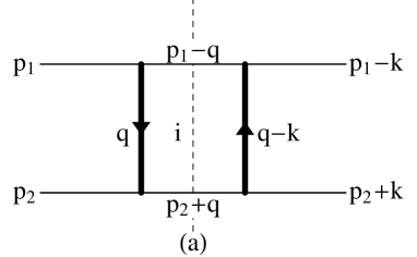
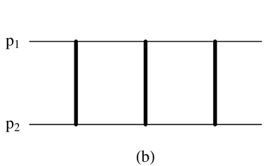
Figure 1: (a) The one-loop contribution corresponding to exchange of two KK modes. The KK modes are drawn as thick lines and standard model particles as thin lines. (b) The two-loop contribution.

The one-loop diagram in fig. 1a is given by the following expression:

$$A_{\rm{1-loop}}(k^{2})=\frac{-i}{2}\int\frac{d^{4}q}{(2\pi)^{4}}A_{\rm{Born}}(q^{2})A_{\rm{Born}}((k-q)^{2})\frac{1}{(p_{1}-q)^{2}}\frac{1}{(p_{2}+q)^{2}}.$$ (11)

Here $p_{1}$ and $p_{2}$ denote the momenta of the incoming particles, the total momentum exchange is $k$ and the loop momentum $q$.

The imaginary part of the integral in eq. (11) is coming from on-shell intermediate states (denoted $i$ in fig. 1), and can be calculated using the Cutcosky cutting rules. This implies that the two propagators in eq. (11) are replaced by $\delta$-functions, which (with the approximation $q^{2}\approx\bar{q}_{\perp}^{2}$) gives the result

$$A_{\rm{1-loop}}(k^{2})=\frac{i}{4s}\int\frac{d^{2}\bar{q}_{\perp}}{(2\pi)^{2}}A_{\rm{Born}}(-\bar{q}_{\perp}^{2})A_{\rm{Born}}(-(\bar{k}_{\perp}-\bar{q}_{\perp})^{2}).$$ (12)

If $A_{\rm{Born}}$ falls off for large $k_{\perp}$, the Fourier transform to impact parameter space of the one-loop contribution is proportional to $\chi^{2}(\bar{b}_{\perp})$. The sum over multi-loop ladder diagrams with different number of KK exchanges exponentiates to $(i\chi-\chi^{2}/2+...)=e^{i\chi}-1$, and the all order eikonal amplitude is given by

$$A_{\rm{eik}}(k^{2})=-2is\int d^{2}\bar{b}_{\perp}e^{i\bar{k}_{\perp}\cdot\bar{b}_{\perp}}(e^{i\chi}-1).$$ (13)

With the Born amplitude in eq. (9) we have, however, some problems. First the real part of the integral in eq. (11) is not small and negligible compared to the imaginary part. It is strongly divergent for $n\geq 2$, as $A_{\rm{Born}}$ increases proportional to $q^{n-2}$ or $q^{n-2}\ln(-q^{2})$ for large $q$. Secondly the integral in eq. (12) should only go over physical intermediate states, which means $q_{\perp}<\sqrt{s}/2$. The Fourier transform of the convolution in eq. (12) gives $\chi^{2}$ only if the integrand in eq. (12) falls off so rapidly, that the integral effectively can be extended to all $q_{\perp}$. This is not the case with the amplitude in eq. (9).

We conclude that, although the result in eq. (10) and (1) is an intuitively reasonable result for scattering in a rapidly falling potential, it should be worrying that it is derived from an amplitude, which grows for large momentum transfers and large scattering angles, while the eikonal approximation is proven to be valid only when scattering at small angles is dominating.

At the root of this problem lies the fact that the subtraction, which gives the amplitude in eq. (9) and is a result of the analytic continuation in the number of extra dimensions, does not automatically remove all parts corresponding to $\delta$-functions at $\bar{r}=0$. The definition of the potential as the Fourier transform of eq. (9) is problematic. To illustrate this we study the most simple example represented by the case $n=3$. In the rest frame we have $k_{0}=0$ and $k^{2}=-\bar{k}^{2}$. The integral in eq. (8) is then proportional to

$$\int\frac{m^{2}\,dm}{\bar{k}^{2}+m^{2}} = \int\frac{(m^{2}+\bar{k}^{2}-\bar{k}^{2})dm}{\bar{k}^{2}+m^{2}}=\int dm-\bar{k}^{2}\int\frac{dm}{\bar{k}^{2}+m^{2}}$$ (14)

$$= \int dm-|\bar{k}|\int\frac{dx}{1+x^{2}}=\int dm-|\bar{k}|\frac{\pi}{2}.$$

The first term, the integral, represents an infinite subtraction. Its three-dimensional Fourier transform gives a $\delta$-function at $\bar{r}=0$ with an infinite weight. The second term corresponds to the result in eq. (9). We may try to define its Fourier transform $\hat{V}(\bar{r})$ as a distribution in the standard way, multiplying with a test function and interchanging the order of integration. For test functions of the form $\exp(-a\,r^{2})$ we then get (with $k\equiv|\bar{k}|$ and the constant $C$ appearing in eq. (25))

$$\int d^{3}re^{-a\,r^{2}}\hat{V}(\bar{r}) \equiv C(-\frac{\pi}{2})\int d^{3}k\,k\int d^{3}re^{-a\,r^{2}}e^{i\bar{r}\bar{k}}$$ (15)

$$= -C\frac{\pi}{2}\int d^{3}k\,ke^{-k^{2}/4a}(\frac{\pi}{a})^{\frac{3}{2}}$$

$$= -C16\pi^{\frac{7}{2}}\sqrt{a}.$$

We note that this result is finite, and goes towards 0 when the test function approaches a constant, i.e. when $a\rightarrow 0$. For $r\neq 0$ we find $\hat{V}(r)=C4\pi^{2}/r^{4}$ by Fourier transforming from $\bar{k}$ to $\bar{r}$ using a convergence factor. Integrating this contribution with the test function above, we get the divergent result

$$C16\pi^{3}\int_{0}^{\infty}e^{-a\,r^{2}}\frac{dr}{r^{2}}.$$ (16)

Thus this definition, $\hat{V}(r)=C4\pi^{2}/r^{4}$ for $r>0$, is incomplete since the result in eq. (15) is finite while the integral in eq. (16) is infinite. It looks as if a $\delta$-function, $\delta(\bar{r})$, with infinite weight is missing.

We conclude that the separation in eq. (14) does not in itself remove all terms related to $\delta$-functions at $\bar{r}=0$. Instead we argue in the next section that dynamical effects will remove the divergencies and give finite results.

In the next section we will consider possible mechanisms, which can suppress high KK masses and give an effective cut-off to the integral in eq. (8). These mechanisms have real dynamical motivations, and we will see that such finite cut-offs do remove all divergences and give well-defined results. For high energies the Born amplitude indeed falls off for large momentum transfers, and the eikonal approximation is applicable. For lower energies this is not the case, and we will in secs. 4 - 6 discuss the resulting amplitudes and cross sections for different relations between the energy, the Planck mass, and the cut-off scale.

3 Possible solutions

In the ADD-model the standard model particles are assumed to live on a thin brane. The mechanism behind this assumption could possibly be taken from string theory [3], but is not a part of the ADD-model itself. The problems discussed in the previous section are related to contributions from KK modes with very high masses. In a relativistic quantized theory there are also formal problems with an infinitely thin and infinitely rigid brane. If the brane is not infinitely thin, but has a finite width, this will effectively suppress the coupling to high-mass KK modes, with wavelengths shorter than the brane width. If the brane really is infinitely thin, then it must be impossible to determine its position with infinite accuracy. In [18, 19] it is demonstrated that the fluctuations in the position of the brane suppresses high-mass KK modes, in a way similar to the effect of a finite brane width. The emission or absorption of a KK mode gives a recoil to the brane, and the fluctuations in the location of the brane can then be regarded as a result of an effective ”surface tension” in the brane.

Let us for definiteness study the effect of the assumption that the standard model fields penetrate a finite distance into the extra dimensions, which gives an effective finite width to the brane [20]. (The possibility of fluctuating branes, studied in [18, 19], give similar results, albeit with a different physical interpretation.) To be specific we assume a Gaussian extension, but this assumption is not essential for our conclusions. Thus we assume the standard model fields to have a wave function with the extension

$$\psi(\overline{y})=\left(\frac{M_{s}}{\sqrt{2\pi}}\right)^{\frac{n}{2}}e^{-\overline{y}^{2}M_{s}^{2}/4}$$ (17)

into the extra dimensions, with $\overline{y}$ denoting the coordinate in the extra dimensions. The overlap between two standard model fields and a KK mode of mass $m$ (what we have in a vertex) is then proportional to

$$\int d\overline{y}\,e^{i\overline{m}\cdot\overline{y}}\left(\frac{M_{s}}{\sqrt{2\pi}}\right)^{2\frac{n}{2}}e^{-\overline{y}^{2}M_{s}^{2}/2}=e^{-m^{2}/(2M_{s}^{2})}$$ (18)

or, in other words, the squared absolute value of the wave function in $\overline{y}$-space Fourier transformed to $m$-space. The exchange of a KK mode will have this suppression factor occurring twice, once at every vertex. In total the exchange of a KK mode with mass $m$ will therefore contribute to the sum in eq. (8) with a suppression factor

$$e^{-m^{2}/M_{s}^{2}}.$$ (19)

Implementing the physical requirement that the standard model particles live on a narrow brane does therefore in itself imply a finite “effective” propagator,

$$R^{n}S_{n}\int\frac{dm\,m^{n-1}}{k^{2}-m^{2}}e^{-m^{2}/M_{s}^{2}}$$ (20)

for the exchange of 4-momentum $k$. (The factor $R^{n}$ comes from the density of KK modes and $S_{n}=2\pi^{n/2}/\Gamma(n/2)$ is the unit surface of a sphere in $n$ dimensions.) We note in particular that this expression (in contrast to the expression in eq. (9)) falls off like $1/k^{2}$ for large momentum transfers, such that $-k^{2}\gg M_{s}^{2}$. This implies that for high energies, $s\gg M_{s}^{2}$, t-channel interaction is dominated by small values of $-k^{2}/s$, i.e. by small angles.

In the following sections we will show that the Fourier transform of the propagator in eq. (20) gives a potential, which falls off $\propto 1/r^{n+1}$ for distances larger than the brane width, given by $1/M_{s}$, and smaller than the compactification radius. Outside this range, both for $r<1/M_{s}$ and for $r>2\pi R$ (where the massless graviton dominates), it varies $\propto 1/r$. We will also study the resulting scattering cross sections under different kinematic conditions.

4 The Born term

4.1 Amplitude

As described in section 3, several physical mechanisms result in effective cut-offs for high masses in the KK propagator. After multiplying eq. (20) by the coupling $4\pi G_{N(4)}$, contracting Lorentz indices (not explicitly included here), and using the relation $G_{N(4)}^{-1}=8\pi R^{n}M_{D}^{2+n}$ we get the following result for the Born amplitude for ultra-relativistic small angle scattering:

$$A_{\rm{Born}}(t)=\frac{s^{2}}{M_{D}^{n+2}}\,S_{n}\int_{0}^{\infty}\frac{dm\,m^{n-1}}{k^{2}-m^{2}}\,e^{-m^{2}/M_{s}^{2}}.$$ (21)

For large angels there are less important corrections from spin polarization which we neglect here and in the following. This integral is convergent and finite for all negative values of $k^{2}=t$ (including 0 when $n\geq 3$). It is easy to find the result in the limits of large and small (negative) $t$-values.

• Large momentum transfers; $-t\gg M_{s}^{2}$

  When $-t$ is large compared to $M_{s}^{2}$, the term $m^{2}$ in the denominator in eq. (21) can be neglected, which gives the result:

  $$A_{\rm{Born}}(t)\approx\frac{s^{2}}{M_{D}^{n+2}}\,S_{n}\int_{0}^{\infty}\frac{dm\,m^{n-1}}{t}e^{-m^{2}/M_{s}^{2}}=\pi^{n/2}\left(\frac{M_{s}}{M_{D}}\right)^{n}\frac{s^{2}}{M_{D}^{2}\cdot t}.$$ (22)

  Thus for large momentum transfers (larger than the cut-off) the Born amplitude falls off proportional to $1/t$.

• Small momentum transfers; $-t\ll M_{s}^{2}$

  For smaller $t$, and $n>2$, the integral is dominated by $m$-values of the order of $M_{s}$, and therefore $t$ can now be neglected in the denominator. We then get the approximately constant result:

  $$A_{\rm{Born}}(t) \approx \frac{-s^{2}}{M_{D}^{n+2}}\,S_{n}\int_{0}^{\infty}dm\,m^{n-3}\,e^{-m^{2}/M_{s}^{2}}$$ (23)

  $$= -\frac{2\pi^{n/2}}{(n-2)}\left(\frac{M_{s}}{M_{D}}\right)^{n}\frac{s^{2}}{M_{D}^{2}M_{s}^{2}}.$$

  Thus for momentum transfers, which are small compared to the cut-off, the Born amplitude is approximately constant for $n>2$. For $n=2$ the result for small $t$ has instead a slowly varying logarithmic dependence, proportional to $\ln(-M_{s}^{2}/t)$.

4.2 Potential

To get the classical non-relativistic potential we start directly from the effective propagator in eq. (20) multiplied with the coupling constant $4\pi G_{N(4)}$. Going to the rest frame, where $k_{0}=0$ and $t=-\bar{k}^{2}$ we find the corresponding potential as the three-dimensional Fourier transform:

$$\frac{V(r)}{m_{1}m_{2}} = \frac{1}{2s^{2}}\int\frac{d^{3}\overline{k}}{(2\pi)^{3}}\,e^{i\bar{k}\bar{r}}A_{\rm{Born}}(-\bar{k}^{2})$$ (24)

$$= \frac{-1}{2M_{D}^{n+2}}\frac{S_{n}}{(2\pi)^{3}}\int_{0}^{\infty}dm\,m^{n-1}\,e^{-m^{2}/M_{s}^{2}}\int\frac{d^{3}ke^{i\bar{k}\bar{r}}}{m^{2}+\bar{k}^{2}}=$$

$$= \frac{-1}{2M_{D}^{n+2}}\frac{S_{n}}{(2\pi)^{3}}2\pi^{2}\int_{0}^{\infty}dm\,m^{n-1}e^{-m^{2}/M_{s}^{2}}\cdot\frac{e^{-mr}}{r}.$$

This represents a weighted sum of Yukawa potentials. The integral can be expressed in terms of error functions, but we are here primarily interested in the behavior for large and small values of $r$.

• Large distances; $r>1/M_{s}$

  For distances larger than the brane thickness the integral is effectively cut off by the factor $e^{-mr}$, and the result becomes insensitive to the Gaussian cut-off $e^{-m^{2}/M_{s}^{2}}$. It is then approximated by

  $$\frac{V(r)}{m_{1}m_{2}}\approx\frac{-1}{2M_{D}^{n+2}}\frac{S_{n}}{4\pi}\int_{0}^{\infty}dmm^{n-1}\cdot\frac{e^{-mr}}{r}=\frac{-S_{n}\,\Gamma(n)}{8\pi M_{D}^{n+2}}\cdot\frac{1}{r^{n+1}}.$$ (25)

  We see that for distances large compared to the brane thickness (but small compared to the compactification radius) we recover the result from eq. (1), a potential falling off proportional to $1/r^{n+1}$, corresponding to the expected ($3+n$)-dimensional version of Newton’s law. When $r$ is increased, smaller $m$-values $\sim 1/r$ are important in the integral in eq. (24) or (25). The phase space factor $m^{n-1}$ then gives this power-like fall off for distances large compared to $M_{s}$.

• Short distances; $r<1/M_{s}$

  For smaller $r$-values we find instead that the factor $e^{-mr}$ is irrelevant, and the result is

  $$\frac{V(r)}{m_{1}m_{2}}=\frac{-1}{2M_{D}^{n+2}}\frac{S_{n}}{4\pi}\frac{1}{r}\int_{0}^{\infty}dm\,m^{n-1}\,e^{-m^{2}/M_{s}^{2}}=\frac{-\pi^{n/2}}{8\pi}\frac{M_{s}^{n}}{M_{D}^{n+2}}\cdot\frac{1}{r}.$$ (26)

  Due to the cut-off, the integral in eq. (24) is dominated by $m$-values close to $M_{s}$ for all $r$-values smaller than $1/M_{s}$. Thus, when the distance is smaller than the brane width, the result is a potential proportional to $1/r$, corresponding to a standard 3-dimensional Coulomb potential, although with a coupling constant $\sim M_{s}^{n}/M_{D}^{n+2}\sim(M_{s}R)^{n}G_{N(4)}$ instead of $G_{N(4)}$. Thus the coupling is enhanced by a factor $\sim(M_{s}R)^{n}=(\frac{\rm{compactification\ radius}}{\rm{brane\ width}})^{n}$.

4.3 Eikonal

In a similar way we can calculate the eikonal $\chi(b)$ by a two-dimensional Fourier transform in the transverse coordinates:

$$\chi(b) = \frac{1}{2s}\int\frac{d^{2}\bar{k}_{\perp}}{(2\pi)^{2}}\,e^{i\bar{k}_{\perp}\bar{b}_{\perp}}A_{\rm{Born}}(-\bar{k}_{\perp}^{2})=$$ (27)

$$= \frac{-s}{2M_{D}^{n+2}}\frac{S_{n}}{(2\pi)^{2}}\int_{0}^{\infty}dm\,m^{n-1}\,e^{-m^{2}/M_{s}^{2}}\int d^{2}\bar{k}_{\perp}e^{i\bar{k}_{\perp}\bar{b}_{\perp}}\frac{1}{m^{2}+\bar{k}_{\perp}^{2}}=$$

$$= \frac{-s}{2M_{D}^{n+2}}\frac{S_{n}}{(2\pi)^{2}}2\pi\int_{0}^{\infty}dm\,m^{n-1}e^{-m^{2}/M_{s}^{2}}\int_{0}^{\infty}\frac{k_{\perp}dk_{\perp}}{m^{2}+k_{\perp}^{2}}\,J_{0}(k_{\perp}b)=$$

$$= \frac{-s}{2M_{D}^{n+2}}\frac{S_{n}}{2\pi}\int_{0}^{\infty}dm\,m^{n-1}e^{-m^{2}/M_{s}^{2}}K_{0}(mb).$$

This integral can be expressed in terms of confluent hypergeometric functions of the second kind:

$$\chi(b)=-\frac{sM_{s}^{n}}{M_{D}^{n+2}}\Gamma(\frac{n}{2})\frac{\pi^{n/2-1}}{8}U(\frac{n}{2},1,\frac{M_{s}^{2}b^{2}}{4}).$$ (28)

This expression can easily be used in numerical calculations. For an intuitive picture, the result for large and small $b$-values can be estimated in the same way as the approximations in eqs. (25, 26).

• Large impact parameters; $b\gg 1/M_{s}$

  For large arguments the asymptotic behavior of the Bessel function $K_{0}(mb)$ is proportional to $\exp(-mb)/\sqrt{mb}$. This implies that for large $b$ the Gaussian cut-off is unessential, and we find the eikonal

  $$\chi(b) \approx \frac{-s}{2M_{D}^{n+2}}\frac{S_{n}}{2\pi}\int dm\,m^{n-1}\,K_{0}(mb)=\frac{-s}{M_{D}^{n+2}}\frac{S_{n}}{\pi}2^{n-4}\,\Gamma^{2}(n/2)\cdot\frac{1}{b^{n}}$$ (29)

  $$= \frac{-s}{2M_{D}^{n+2}}(4\pi)^{\frac{n}{2}-1}\Gamma\left(\frac{n}{2}\right)\cdot\frac{1}{b^{n}}.$$

• Small impact parameters; $b\ll 1/M_{s}$

  For small arguments we have $K_{0}(mb)\approx\ln(1/(mb))$, which implies

  $$\chi(b) \approx \frac{-s}{2M_{D}^{n+2}}\frac{S_{n}}{2\pi}\int dm\,m^{n-1}\,e^{-m^{2}/M_{s}^{2}}\ln\left(\frac{1}{mb}\right)$$ (30)

  $$= \frac{\pi^{\frac{n}{2}-1}}{4}\frac{s}{M_{D}^{2}}\left(\frac{M_{s}}{M_{D}}\right)^{n}\left(\ln(M_{s}b)+\frac{1}{2}\psi(\frac{n}{2})\right)$$

  where $\psi(\frac{n}{2})$ is the psi or digamma function.

Thus we see that the eikonal falls off $\propto 1/b^{n}$ for large $b$, and grows logarithmically when $b\rightarrow 0$. Using the quantity $b_{c}$ from eq. (10) and keeping only the dominant term $\ln(M_{s}b)$ in eq. (30), we can write the results in the form

$$\chi(b) \approx -\left(\frac{b_{c}}{b}\right)^{n};\,\,\,b>b_{d}$$ (31)

$$\chi(b) \approx \frac{-(b_{c}\,M_{s})^{n}}{2^{n-1}\Gamma(n/2)}\ln\left(\frac{1}{M_{s}b}\right);\,\,\,b<b_{d}$$ (32)

$$\mathrm{with}\,\,\,b_{d} \equiv \frac{1}{M_{s}}$$ (33)

$$\,\,\mathrm{and}\,\,b_{c} \equiv \left[\frac{s(4\pi)^{\frac{n}{2}-1}\Gamma(n/2)}{2M_{D}^{n+2}}\right]^{1/n}.$$ (34)

The separation line $b_{d}=1/M_{s}$ is an estimate of the $b$-value where $\chi(b)$ changes behavior. As an example fig. 2 shows these approximations for $\chi$ together with the exact result for $n=3$ and $\sqrt{s}=M_{D}=1$ in units such that $M_{s}=1$. As $\chi$ is proportional to $s/M_{D}^{n+2}$, a change in $s$ and/or $M_{D}$ just corresponds to a shift of all curves the same distance up or down.

Figure 2: The logarithm of $|\chi|$ as a function of impact parameter for $n=3$. The curves show the example where $\sqrt{s}$, $M_{D}$, and $M_{s}$ have the same magnitude, and the units are chosen such that $\sqrt{s}=M_{D}=M_{s}=1$. This also implies that $b_{d}=1$. The uppermost line is the large $b$ limit of $\chi$ taken from eq. (31) and the lowermost line is the small $b$ limit of $\chi$ taken from eq. (32). The interpolating line is the exact expression eq. (28). Note that a change in $s$ and/or $M_{D}$, keeping $M_{s}$ constant, just corresponds to shifting all curves up or down.

5 Higher order loop corrections

We note that three different energy scales enter the expressions for the Born amplitude in eqs. (21, 28): $\sqrt{s}$, $M_{D}$, and $M_{s}$. Here $\sqrt{s}$ is the total energy in the scattering, $M_{D}$ is the fundamental Planck scale determined by the compactification radius $R$, and $M_{s}$ is related to the width of the brane (or the brane tension). The result depends on the relative magnitude of these quantities, and in the following we will successively discuss five different kinematical regions, which are illustrated in fig. 3.

Figure 3: The $(\sqrt{s},M_{s})$-plane for $n=3$ and $M_{D}=1$. The straight line separating region 1 and 4 is $\sqrt{s}=M_{s}$ while straight line separating region 4 and 5 is the line where the real and imaginary parts in eq. (38) have equal magnitude. The power-like curve separating region 1 and 2 is $s_{cd}$ from eq. (36) as a function of $M_{s}$ and the line separating the regions 4 and 5 from region 3 is the line where $|A_{\rm{Born}}X|=1$, see eq. (38). In the regions 1 and 2 $s$ is larger than $M_{s}$, and, at least for $s\gg M_{s}$, the eikonal approximation is correct. In region 1 the eikonal is, depending on $b$, either large compared to 1 or given by eq. (31). In region 2 on the other hand the $b$-range where $\chi$ is small includes a region where it is described by eq. (32). In region 3 the correction corresponding to higher order loops is small, but in region 4 it is important to assure unitarity.

5.1 Eikonal regions, $s\gg M_{s}^{2}$

We study the scattering process in the overall cm system, where the momentum exchange has no 0-component, $k=(0;\bar{k})$ and $t=-\bar{k}^{2}$. From eq. (22) we see that $A_{\rm{Born}}$ falls off $\propto 1/\bar{k}^{2}$ for $\bar{k}^{2}>M_{s}^{2}$. Thus for high energies, such that $s\gg M_{s}^{2}$, corresponding to region $1$ and $2$ in fig. 3, the Born term is dominated by small values of $\bar{k}^{2}/s$, i.e. small angles. This implies that the eikonal approximation is applicable. We note in particular that it is $M_{s}$ rather than $M_{D}$, that sets the scale for when the eikonal approximation is relevant. The one-loop contribution is here dominated by its imaginary part, obtained when the particles in the intermediate state $i$ in fig. 1a are on shell. The contributions from multi-loop ladder diagrams (fig. 1b) exponentiate, and the scattering amplitude is given by eq. (13):

$$A_{\rm{eik}}(k^{2})=2is\int d^{2}\bar{b}_{\perp}e^{i\bar{k}_{\perp}\cdot\bar{b}_{\perp}}(1-e^{i\chi}).$$ (35)

From eq. (35) we see that the higher order corrections are important when $\chi$ is of order 1 or larger. Correspondingly the Born term dominates when $|\chi|<1$. We see from eqs. (32, 33) that $\chi$ varies only logarithmically when $b$ is decreased below the point $b=b_{d}$. The importance of the higher order corrections for the integrated cross section therefore depends on whether or not $|\chi(b_{d})|>1$. This relation is satisfied whenever $b_{c}>b_{d}$, or equivalently when $s>s_{cd}$, with $s_{cd}$ given by

$$s_{cd}=\frac{2}{(4\pi)^{\frac{n}{2}-1}\Gamma(\frac{n}{2})}\frac{M_{D}^{n+2}}{M_{s}^{n}}.$$ (36)

This defines the boundary between region 1 and region 2 in fig. 3. In region 1 higher order terms are important for $b<b_{c}$, and the exponentiation in eq. (35) is essential to keep the amplitude within the unitarity constraints.

The difference between regions 1 and 2 is illustrated in fig. 4. Fig. 4a corresponds to region 1, where the energy is high, and $b_{c}>b_{d}$. The absolute value of the eikonal $\chi$ is smaller than 1 for $b>b_{c}$, and in this range the approximation in eq. (31) is relevant. For $b<b_{c}$, $|\chi|$ is large and rapidly varying, which causes the exponent in eq. (35) to oscillate rapidly.

Fig. 4b corresponds to region 2. Here $|\chi|<1$ except in a very small region

$$b<\frac{1}{M_{s}}\exp\left(-\frac{4M_{D}^{n+2}\pi^{1-\frac{n}{2}}}{sM_{s}^{n}}\right)$$ (37)

around the origin. Therefore the Born term dominates the cross section, and higher order terms give only small corrections.

Figure 4: $-\chi$ as a function of impact parameter for two examples with $n=3$. (a) High energies corresponding to region 1 in fig. 3, with $\sqrt{s}=10$ TeV, $M_{s}=1$ TeV and $M_{D}=1$ TeV. The upper curve is the approximate expression in eq. (29), and the lower curve the exact expression eq. (38). (b) Kinematics corresponding to region 2 in fig. 3, $\sqrt{s}=0.1$ TeV $M_{s}=1$ TeV and $M_{D}=1$ TeV. The upper curve is the approximate high $b$ expression in eq. (31), the lower curve the approximate low $b$ expression in eq. (32) and the interpolating line is the exact expression in eq. (28).

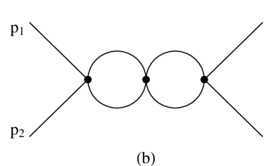
Figure 5: When the exchanged momentum is small compared to $M_{s}$, the KK propagators are effectively replaced by vertex factors. The diagrams in fig. 1 can then be drawn as above with only standard model particle lines.

5.2 Non-eikonal regions, $s<M_{s}^{2}$

The Born amplitude in eq. (23) is almost independent of the momentum exchange $\bar{k}$ when $k\ll M_{s}$. When $\sqrt{s}\ll M_{s}$ (regions $3$, $4$, and 5 in fig. 3) this includes all kinematically allowed $\bar{k}$-values, which implies that the scattering is almost isotropic. Thus the exchange of the KK modes corresponds effectively to a contact interaction. (For wide-angle scattering we also expect corrections from spin polarization. This effect is neglected in the following.) The one-loop contribution in fig. 1a is then represented by the diagram in fig. 5a, which is easily calculated. We denote the momenta in the intermediate state $P/2\pm q$, with $P=p_{1}+p_{2}$, as indicated in fig. 5a, and in the cms we have $P=(W,\bar{0})$. The vertices are then given by the Born term in eq. (23), with an effective cut-off when $q=M_{s}$. The result is therefore

$$A_{\rm{1-loop}}(k^{2}) = \frac{-i}{2}\int_{k<M_{s}}\frac{d^{4}q}{(2\pi)^{4}}A_{\rm{Born}}^{2}\frac{1}{(P/2-q)^{2}}\frac{1}{(P/2+q)^{2}}=$$ (38)

$$\equiv A_{\rm{Born}}^{2}\cdot X,\,\,\,\,\mathrm{with}\,\,X\approx\frac{1}{32\pi^{2}}(\ln\frac{4M_{s}^{2}}{s}+i\pi)$$

We note here in particular that the result is a constant, independent of the momentum transfer $k$. Therefore also the one-loop amplitude can be effectively regarded as a contact term with a cut-off when $k>M_{s}$. Consequently the two-loop diagram in fig. 5b can be calculated in the same way as the one-loop diagram, and the result is

$$A_{\rm{2-loop}}=A_{\rm{1-loop}}\cdot A_{\rm{Born}}X=A_{\rm{Born}}\cdot(A_{\rm{Born}}X)^{2}.$$ (39)

In the same way we can calculate ladder diagrams with more loops. Summing all ladders we obtain

$$A_{\mathrm{ladder}}=A_{\rm{Born}}\,(1+A_{\rm{Born}}X+(A_{\rm{Born}}X)^{2}+\ldots\ )=\frac{A_{\rm{Born}}}{1-A_{\rm{Born}}X}.$$ (40)

We see that instead of the exponent in the eikonal regime (where forward scattering dominates) we here obtain a geometric series from ladder type contributions. The importance of higher order corrections is now determined by the quantity $A_{\rm{Born}}\,X$. When $|A_{\rm{Born}}\,X|\ll 1$ the Born term dominates. This corresponds to region 3 in fig. 3.

When instead $|A_{\rm{Born}}\,X|>1$, we expect different results depending on whether it is the real or the imaginary part which dominates. When $\ln(4M_{s}^{2}/s)<\pi$, the imaginary part dominates the loop integral in eq. (38). Thus this diagram is dominated by real intermediate states $i$ in fig. 1a, and the ladder diagrams in fig. 1b or fig. 5b should be important higher order corrections. This corresponds to region 4 in fig. 3.

When $\ln(4M_{s}^{2}/s)>\pi$ (region 5 in fig. 3) the real part dominates the loop integral. This implies that inelastic scattering and virtual intermediate states are essential. We then expect important contributions from more complicated, non-ladder, diagrams, like the examples shown in fig. 6. For this reason we do not expect the result in eq. (40) to be representative for a sum of all higher order corrections in this kinematical region.

Figure 6: (a) An example of a non-ladder diagram contributing to the elastic cross section in region 5 in fig. 3. (b) An example of a diagram contributing to the inelastic cross section in region 5 in fig. 3.

6 Cross sections

Below we successively discuss the cross sections obtained in the five different regions in fig. 3.

6.1 Region 1, $s>M_{s}^{2}$ and $|\chi(b_{d})|>1$

In this region $s>M_{s}^{2}$ and $\chi(b_{d})>1$. As discussed in section 5.1 the scattering is suppressed for $-t>M_{s}^{2}$. The first constraint therefore means that the cross section is dominated by small angle scattering, the imaginary part dominates the one-loop contribution, and the eikonal $\chi(b)$ exponentiates. The cross section is then given by

$$\sigma=\int d^{2}\bar{b}_{\perp}\,2Re(1-e^{i\chi(\bar{b}_{\perp})}).$$ (41)

The effect of the constraint $|\chi(b_{d})|>1$ was illustrated in fig. 4a. It implies that $b_{d}<b_{c}$, and that the approximation $\chi\approx-(b_{c}/b)^{n}$ in eq. (31) is relevant for all $b>b_{c}$. In particular this means that, for $b>b_{c}\,(>b_{d})$, we have $|\chi|<1$ and $2Re(1-e^{i\chi(\bar{b}_{\perp})})\approx\chi^{2}$. For central collisions, where $b<b_{c}$, higher order loop corrections are important to satisfy unitarity. Here $|\chi|$ is larger than 1 and rapidly varying, the exponent in eq. (41) is oscillating, and therefore

$$\left<\,2Re(1-e^{i\chi(\bar{b}_{\perp})})\,\right>\,\approx 2.$$ (42)

(For $b<b_{d}$ the variation in $\chi$ is only logarithmic, and therefore small in relative magnitude. As $\chi$ is very large, the variation may still be large in absolute magnitude and such that eq. (42) is valid also here.) Inserting these results into eq. (41), we get (for $n\geq 2$) the following result for the total cross section:

$$\sigma\approx\int_{0}^{b_{c}}d^{2}b\cdot 2+\int_{b_{c}}^{\infty}d^{2}b\left(\frac{b_{c}}{b}\right)^{2n}=\pi b_{c}^{2}(2+\frac{1}{n-1})=2\pi\,b_{c}^{2}\,\frac{n-1/2}{n-1}.$$ (43)

When $s$ is increased, $\sigma$ grows proportional to $b_{c}^{2}\propto s^{2/n}$. We note that the cross section is dominated by central collisions with $b<b_{c}$ (especially for large $n$), with only a small contribution from larger impact parameters. Integrating the constant 1 in the parenthesis in eq. (35) between 0 and $b_{c}$ gives a dominant forward peak, with oscillations at larger angles. The amplitude for these oscillations falls off proportional to $1/k^{3/2}$, corresponding to $d\sigma/dt\propto 1/k^{3}$ for the cross section.

For large $k$ the dominant contribution in eq. (35) comes from the term $e^{i\chi}$ and a small range of $b$-values around $b_{s}$, where

$$b_{s}=b_{c}\left(\frac{n}{kb_{c}}\right)^{\frac{1}{n+1}}.$$ (44)

For these $b$-values the frequencies of the exponents $e^{i\overline{k}\cdot\overline{b}}$ and $e^{i\chi(\overline{b})}$ in eq. (35) oscillate in phase, which gives an enhanced contribution. Using the saddle-point approximation we get from this contribution (apart from logarithmic corrections) a cross section which falls off like $d\sigma/dt\propto 1/t^{\frac{n+2}{n+1}}$. This contribution is dominating for $k>n/b_{c}$, where $|\chi(b_{s})|>1$. As pointed out in [4] it corresponds to classical scattering in a $1/r^{n+1}$-potential. For small scattering angles $\theta$ we have for a non-relativistic particle with mass $m_{1}$ moving with constant speed $v$ and momentum $p=m_{1}v$ in the potential of a mass $m_{2}$

$$\theta\approx\frac{|\bar{p}_{\perp}|}{|\overline{p}|} = \frac{1}{|\overline{p}|}\int_{-\infty}^{\infty}dtF_{\perp}(r)$$

$$= -G_{N(4)}R^{n}S_{n}\Gamma(n)\frac{m_{1}m_{2}}{m_{1}v}\int_{-\infty}^{\infty}\frac{dr}{v}\frac{d}{db}\left(\frac{1}{\sqrt{r^{2}+b^{2}}}\right)^{n+1}$$

$$= \frac{n(2\sqrt{\pi})^{n}\Gamma(\frac{n}{2})}{8\pi v^{2}}\frac{m_{2}}{M_{D}^{n+2}}\frac{1}{b^{n+1}}.$$

From this we see that if $m_{1}=s/(4m_{2})$

$$b_{\rm{nonrel}}=b_{c}\left(\frac{n}{4vpb_{c}}\right)^{\frac{1}{n+1}}$$ (46)

agreeing parametrically with eq. (44). (A numerical difference is expected since eq. (44) is ultra-relativistic whereas eq. (46) is a non-relativistic result.) This behavior is discussed in more detail in [4], and we note that in this region, where $s$ is much larger than both $M_{s}^{2}$ and $s_{cd}$, our result is consistent with the result of this reference. A necessary condition is, however, that $\sqrt{s}$, $M_{D}$, and $M_{s}$ have values such that $b_{s}>b_{d}=1/M_{s}$, which for fixed $k$-value gives a minimum value for $M_{s}$. If this relation is not satisfied, the phase variation in $\exp(i\chi)$ is given by eq. (32) rather than eq. (31), and therefore we do not get the phase coherence in the integral in eq. (35).

6.2 Region 2, $s>M_{s}^{2}$ and $|\chi(b_{d})|<1$

In region 2, $s$ is larger than $M_{s}^{2}$ but smaller than $s_{cd}$, and therefore $b_{d}>b_{c}$. A typical example is illustrated in fig. 4b. We see here that $|\chi|$ is small compared to 1, apart from the logarithmic peak for very small $b$. The influence of the small $b$ peak is also suppressed by a phase space factor proportional to $b\,db$. The cross section is therefore well approximated by the Born amplitude.

The largest contributions to the cross section come from $b$-values in the neighborhood of $b_{d}$; for larger $b$, $\chi$ falls off $\propto(b_{c}/b)^{n}$, and for smaller $b$ the scattering is limited by the smaller phase space $\sim b\,db$. These $b$-values are just in the transition region between the two asymptotic forms in eqs. (31, 32). To get a good estimate of the cross section we should therefore use the exact expression for $\chi$ in eq. (28). For an order of magnitude estimate we may, however, approximate $\chi$ by the asymptotic result $\chi\approx-(b_{c}/b)^{n}$ for $b>b_{d}$, and by a constant $=-(b_{c}/b_{d})^{n}$ for all $b<b_{d}$. This gives the following qualitative estimate for the total cross section:

$$\sigma\sim\int_{0}^{b_{d}}d^{2}b\left(\frac{b_{c}}{b_{d}}\right)^{2n}+\int_{b_{d}}^{\infty}d^{2}b\left(\frac{b_{c}}{b}\right)^{2n}=\pi\frac{b_{c}^{2n}}{b_{d}^{2n-2}}\,\frac{n}{n-1}.$$ (47)

As $b_{c}\sim(s/M_{D}^{n+2})^{1/n}$, and $b_{d}=1/M_{s}$, we note that the cross section grows $\propto s^{2}M_{s}^{2n-2}/M_{D}^{2n+4}$. Thus, although the cross section is comparatively small in this region, it has a stronger growth rate $\propto s^{2}$ than in region 1.

For the differential cross section, we note that the t-channel Born amplitude is proportional to $1/k^{2}$ for $-k^{2}\gg M_{s}^{2}$. This implies that the cross section has a forward peak. It corresponds to scattering at distances small compared to $1/M_{s}$, in the $1/r$ potential from eq. (26). There is however no forward divergence since the growth is softened at $-k^{2}\sim M_{s}^{2}$, i.e. at distances comparable to the brane thickness.

6.3 Region 3, $s<M_{s}^{2}$ and $|A_{\rm{Born}}X|<1$

In region 3 the cross section is also dominated by the Born amplitude. But in this case the scattering is almost isotropic (apart from spin dependences) as the factor $-k^{2}$ in the propagator is small compared to the heavier and most important KK modes. This implies that we may also have important contributions from u- and s-channel exchanges. For identical particles, the u-channel contribution has the same magnitude as that from t-channel.

6.4 Region 4, $s<M_{s}^{2}$, $|A_{\rm{Born}}X|>1$ and $\mbox{Im}(X)>\mbox{Re}(X)$

The one-loop t-type contribution in fig. 5a, is dominated by the imaginary part, originating from real intermediate states. If loop diagrams of this type dominate, the all-loop amplitude is approximated by the geometric sum in eq. (38). As in region 3, the result is then approximately isotropic, but here higher order corrections give some suppression compared to the Born approximation. For identical particles the u-type ladder is identical to the t-type ladder and hence equally important. For particle-antiparticle scattering s-channel contributions have to be considered.

6.5 Region 5, $s<M_{s}^{2}$, $|A_{\rm{Born}}X|>1$ and $\mbox{Im}(X)<\mbox{Re}(X)$

In this region the one-loop diagram has a dominant real part. This implies that virtual intermediate states and inelastic reactions are important. Therefore non-ladder diagrams are expected to give large contributions, and we showed two examples in fig. 6. This region is consequently much more complicated than the other kinematical regions. It corresponds to situations where the effective cut-off $M_{s}$ is large (”narrow brane” or strong ”brane tension”) and the energy is in an intermediate range. From fig. 3 we see that for, e.g. $n=3$, $M_{s}$ must be larger than 5 $M_{D}$. In this paper we will not make any specific predictions for what might be expected in this kinematic region.

7 Conclusions

In the ADD model it is assumed that standard model particles live on a 4-dimensional brane, embedded in a $(4+n)$-dimensional space with $n$ compactified dimensions. In these only the gravitational field is allowed to propagate. If the brane is infinitely thin and infinitely rigid, the exchange of very massive Kaluza–Klein modes represents a contact interaction of infinite strength between the standard model particles. This is not physically acceptable and different ideas have been proposed to regularize the scattering process.

If the brane has a finite width, or if it is not infinitely well localized, the exchange of KK modes will be suppressed for KK wavelengths shorter than the width of the brane, or the size of its fluctuations. This will therefore give an effective cut-off (denoted $M_{s}$) for high KK masses, which does not have to be of the same magnitude as the fundamental Planck mass $M_{D}$.

In this paper we have studied the effect of such a cut-off on the scattering of standard model particles at various energies. We find that several troublesome infinities and divergencies are removed. The scattering process depends on three different energy scales, the collision energy $\sqrt{s}$, the fundamental Planck scale $M_{D}$, and the cut-off scale $M_{s}$. The Planck scale, $M_{D}=(8\pi R^{n}G_{N(4})^{-1/(n+2)}$, depends on the compactification radius $R$ of the extra dimensions and the magnitude of Newton’s constant, while the effective cut-off depends on the width of the brane, $M_{s}\sim(\mathrm{brane}\ \mathrm{thickness})^{-1}$, or the fluctuations in its position. These scales are thus not automatically related. Clearly the compactification scale $R$ must be larger than the brane width $1/M_{s}$.

Depending on the relative magnitude between these scales, we have here studied five different kinematical regions with different dynamical behavior. In one region (region 1 in fig. 3), the scattering is dominated by small angles, and the eikonal approximation is applicable. Here we recognize classical scattering in a $1/r^{n+1}$ potential and the results of Giudice-Rattazzi-Wells [4]. In two other regions (2 and 3 in fig. 3) the Born approximation is applicable. In one of these (region 2) forward scattering dominates, and corresponds to scattering in a $1/r$ potential, but with a coupling enhanced by a factor proportional to $(\frac{\rm{compactification\ radius}}{\rm{brane\ width}})^{n}$ compared to scattering in the ordinary $1/r$ Newtonian large distance potential. In the other Born region (region 3) the scattering is approximately isotropic, as expected in [5, 6]. In a fourth region the exponentiation from ladder-type diagrams in the eikonal region is replaced by a geometric sum. The scattering is expected to be mostly elastic since on-shell intermediate states dominate, but approximately isotropic. In the last region inelastic processes and non-ladder loop diagrams are important and make predictions very difficult. The boundaries between the different regions are expressed in the three mass scales involved, as illustrated in fig. 3.

References

- [1] N. Arkani-Hamed, S. Dimopoulos, and G. R. Dvali Phys. Lett. B429 (1998) 263–272, hep-ph/9803315.
- [2] N. Arkani-Hamed, S. Dimopoulos, and G. R. Dvali Phys. Rev. D59 (1999) 086004, hep-ph/9807344.
- [3] I. Antoniadis, N. Arkani-Hamed, S. Dimopoulos, and G. R. Dvali Phys. Lett. B436 (1998) 257–263, hep-ph/9804398.
- [4] G. F. Giudice, R. Rattazzi, and J. D. Wells Nucl. Phys. B630 (2002) 293–325, hep-ph/0112161.
- [5] T. Han, J. D. Lykken, and R.-J. Zhang Phys. Rev. D59 (1999) 105006, hep-ph/9811350.
- [6] G. F. Giudice, R. Rattazzi, and J. D. Wells Nucl. Phys. B544 (1999) 3–38, hep-ph/9811291.
- [7] G. F. Giudice and A. Strumia Nucl. Phys. B663 (2003) 377–393, hep-ph/0301232.
- [8] D. Atwood, S. Bar-Shalom, and A. Soni Phys. Rev. D62 (2000) 056008, hep-ph/9911231.
- [9] R. I. Glauber, Lectures in Theoretical Physics. Interscience Publisher, NY, 1959.
- [10] R. Blankenbecler and M. L. Goldberger Phys. Rev. 126 (Apr, 1962) 766–786.
- [11] R. C. Arnold Phys. Rev. 153 (Jan, 1967) 1523–1546.
- [12] R. Emparan, G. T. Horowitz, and R. C. Myers Phys. Rev. Lett. 85 (2000) 499–502, hep-th/0003118.
- [13] S. Dimopoulos and G. Landsberg Phys. Rev. Lett. 87 (2001) 161602, hep-ph/0106295.
- [14] S. B. Giddings and S. Thomas Phys. Rev. D65 (2002) 056010, hep-ph/0106219.
- [15] P. Kanti Int. J. Mod. Phys. A19 (2004) 4899–4951, hep-ph/0402168.
- [16] L. Lönnblad, M. Sjodahl, and T. Akesson JHEP 09 (2005) 019, hep-ph/0505181.
- [17] C. M. Harris and P. Kanti JHEP 10 (2003) 014, hep-ph/0309054.
- [18] M. Bando, T. Kugo, T. Noguchi, and K. Yoshioka Phys. Rev. Lett. 83 (1999) 3601–3604, hep-ph/9906549.
- [19] T. Kugo and K. Yoshioka Nucl. Phys. B594 (2001) 301–328, hep-ph/9912496.
- [20] M. Sjodahl hep-ph/0602138.