Evading Equivalence Principle Violations, Cosmological and other Experimental Constraints in Scalar Field Theories with a Strong Coupling to Matter

Abstract

We show that, as a result of non-linear self-interactions, it is feasible, at least in light of the bounds coming from terrestrial tests of gravity, measurements of the Casimir force and those constraints imposed by the physics of compact objects, big-bang nucleosynthesis and measurements of the cosmic microwave background, for there to exist, in our Universe, one or more scalar fields that couple to matter much more strongly than gravity does. These scalar fields behave like chameleons: changing their properties to fit their surroundings. As a result these scalar fields can be not only very strongly coupled to matter, but also remain relatively light over solar system scales. These fields could also be detected by a number of future experiments provided they are properly designed to do so. These results open up an altogether new window, which might lead to a completely different view of the rôle played by light scalar fields in particle physics and cosmology.

I Introduction

There is wide-spread interest in the possibility that, in addition to the matter described by the standard model of particle physics, our Universe may be populated by one or more scalar fields. These are a general feature in high energy physics beyond the standard model and are often related to the presence of extra-dimensions, morecham3 . The existence of scalar fields has also been postulated as means to explain the early and late time acceleration of the Universe sn1a ; inflation ; quint ; quint1 ; quint2 ; easson . It is almost always the case that such fields interact with matter: either due to a direct Lagrangian coupling or indirectly through a coupling to the Ricci scalar or as the result of quantum loop corrections, damour ; carroll1 ; carroll2 ; anupam1 ; anupam2 . If the scalar field self-interactions are negligible, then the experimental bounds on such a field are very strong: requiring it to either couple to matter much more weakly than gravity does, or to be very heavy uzan ; bounds ; damour1 ; damour2 . Recently, a novel scenario was presented by Khoury and Weltman cham1 that employed self-interactions of the scalar-field to avoid the most restrictive of the current bounds. In the models that they proposed, a scalar field couples to matter with gravitational strength, in harmony with general expectations from string theory, whilst, at the same time, remaining very light on cosmological scales. In this paper we will go much further and show, contrary to most expectations, that the scenario presented in cham1 allows scalar fields, which are very light on cosmological scales, to couple to matter much more strongly than gravity does, and yet still satisfy all of the current experimental and observational constraints.

The cosmological value of such a field evolves over Hubble time-scales and could potentially cause the late-time acceleration of our Universe chameleoncosmology . The crucial feature that these models possess is that the mass of the scalar field depends on the local background matter density. On Earth, where the density is some $10^{30}$ times higher than the cosmological background, the Compton wavelength of the field is sufficiently small as to satisfy all existing tests of gravity. In the solar system, where the density is several orders of magnitude smaller, the Compton wavelength of the field can be much larger. This means that, in those models, it is possible for the scalar field to have a mass in the solar system that is much smaller than was previously thought allowed. In the cosmos, the field is lighter still and its energy density evolves slowly over cosmological time-scales and it could function as an effective cosmological constant. While the idea of a density-dependent mass term is not new added ; pol ; others ; others1 ; others2 ; others3 , the work presented in cham1 ; chameleoncosmology is novel in that the scalar field can couple directly to matter with gravitational strength. If a scalar field theory contains a mechanism by which the scalar field can obtain a mass that is greater in high-density regions than in sparse ones, we deem it to possess a chameleon mechanism and be a chameleon field theory. When referring to chameleon theories, it is common to refer to the scalar field as the chameleon.

We start this article by reviewing the main features of scalar field theories with a chameleon mechanism. Afterwards, this paper is divided into roughly two parts: in sections III, IV and V we study the behaviour of chameleon theories as field theories, and derive some important results. From sections VI onwards, we combine these results with a number of experimental and astrophysical limits to constrain the unknown parameters of these chameleon theories $\{\beta,M,\lambda\}$. We shall show how the non-linear effects, identified in sections III-V, allow for a very large matter coupling, $\beta$, to be compatible with all the available data. We also note that some laboratory based tests of gravity need to be redesigned, if they are to be able to detect the chameleon. If the design of these experiments can be adjusted in the required way, and their current precision maintained of its current level, then a large range of sub-Planckian chameleon theories could be detected, or ruled out, in the near future.

In section III, we study how $\phi$ behaves both inside and outside an isolated body and derive the conditions that must hold for such a body to have a thin-shell. In this section, we show how non-linear effects ensure that the value that the chameleon takes far away from a body with a thin-shell is independent of the matter-coupling, $\beta$. Whilst such $\beta$-independence as been noted before for $\phi^{4}$-theory in nelson , this is the first time that it has been shown to be a generic prediction of a large class of chameleon theories. In section IV we show the internal, microscopic, structure of macroscopic bodies can unexpectedly alter the macroscopic behaviour of the chameleon. Using the results of section III and IV we are then able to calculate the $\phi$-force between two bodies; this is done in section V. In each of these sections we take care to note precisely when linearisation of the chameleon field equation is invalid.

Laboratory bounds on chameleon field theories are analysed in section VI. We focus mainly on the Eöt-Wash experiment reported in EotWash ; Eotnew , which tests for corrections to the $1/r^{2}$ behaviour of gravity, and experimental programmes that measurement the Casimir force Lamcas ; Decca ; othercas . We also look at the variety of laboratory and solar-system based tests for violations of the weak equivalence principle (WEP) LLR ; WEP ; WEP1 ; WEP2 . The extent to which proposed satellite-based searches for WEP violation will aide in the search for scalar fields with a chameleon-like behaviour is considered in this section. We shall see that for a large range of values of $M$ and $\lambda$, laboratory tests of gravity at unable to place any upper-bound on $\beta$.

In sections VII and VIII we show how the stability of white-dwarfs and neutron stars, as well as requirements coming from big bang nucleosynthesis and the Cosmic Microwave Background, can be used to bound the parameters of chameleon field theories. We shall see that such considerations do result in upper-bounds on $\beta$.

Finally, in sections IX and X we collate all of the different experimental and astrophysical restrictions on chameleon theories, use them to plot the allowed values of $\beta$, $M$ and $\lambda$, and discuss our results and their implications.

We include a summary of the main results at the end of sections III-V for easy reference. This allows the reader, less interested on the detailed derivation of the formulae, to follow the whole article. Throughout this work we take the signature of spacetime to be $(+\,-\,-\,-)$ and set $\hbar=c=1$; $G=1/M_{pl}^{2}$ where $M_{pl}$ is the Planck mass.

II Chameleon Field Theories

In the theories proposed in cham1 , the chameleon mechanism was realised by giving the scalar field both a potential, $V(\phi)$, and a coupling to matter, $B(\beta\phi/M_{pl})\rho$; where $\rho$ is the local density of matter. We shall say more about how the functions $V$ and $B$ are defined, and the meaning of $\beta$, below. The potential and the coupling-to-matter combine to create an effective potential for the chameleon field: $V^{eff}(\phi)=V(\phi)+B(\beta\phi/M_{pl})\rho$. The values $\phi$ takes at the minima of this effective potential will generally depend on the local density of matter. If at a minima of $V^{eff}$ we have $\phi=\phi_{c}$, i.e. $V^{eff}_{,\phi}(\phi_{c})=0$, then the effective ‘mass’ ($m_{c}$) of small perturbations about $\phi_{c}$, will be given by the second derivative of $V^{eff}$, i.e. $m_{c}^{2}=V^{eff}_{,\phi\phi}(\phi_{c})$. It is usually the case that $|V_{,\phi\phi}|\gg|B_{,\phi\phi}\rho|$ and so $m_{c}$ will be determined almost entirely by the form of $V(\phi)$ and the value of $\phi_{c}$. If $V(\phi)$ is neither constant, linear nor quadratic in $\phi$ then $V_{,\phi\phi}(\phi_{c})$, and hence the mass $m_{c}$, will depend on $\phi_{c}$. Since $\phi_{c}$ depends on the background density of matter, the effective mass will also be density-dependent. Such a form for $V(\phi)$ inevitably results in non-linear field equations for $\phi$.

For a scalar field theory to be a chameleon theory, the effective mass of the scalar must increase as the background density increases. This implies $V_{,\phi\phi\phi}(\phi_{c})/V_{,\phi}(\phi_{c})>0$. It is important to note that it is not necessary for either $V(\phi)$, or $B(\beta\phi/M_{pl})$, to have any minima themselves for the effective potential, $V^{eff}$, to have minimum. A sketch of the chameleon mechanism, as described above, is shown in FIGS. 1 and 2.

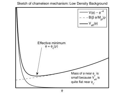
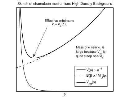
Figure 1: Sketch of the chameleon mechanism for a runaway potential: $V\sim\phi^{-4}$. The sketch on the left is for a low density background, whereas the drawing of the right shows what occurs when there is a high density of matter in the surroundings. We can clearly see that the position of the effective minimum, $\phi_{c}$, and the steepness of the effective potential near that minimum, depends on the density. A shallow minimum corresponds to a low chameleon mass. The mass of the chameleon can be clearly seen to grow with the background density of matter.

In FIG 1 the potential is taken to be of runaway form and has no minimum itself. However, It is clear from the sketches that $V^{eff}$ does have an minimum, and that the value $\phi$ takes at that minimum is density dependent. In FIG 2 the potential is taken to behave like $\phi^{4}$ and so does have a minimum at $\phi=0$. However, the minimum of the effective potential, $V^{eff}$, does not coincide with that of $V$. Once again, the minimum of $V^{eff}$ is seen to be density dependent.

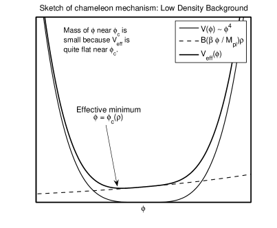
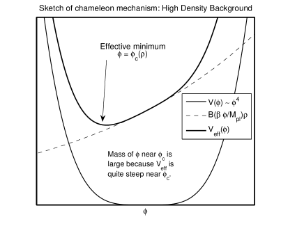
Figure 2: Sketch of the chameleon mechanism for a potential with a minimum at $\phi=0$: $V\sim\phi^{4}$. The sketch on the left is for a low density background, whereas the drawing of the right shows what occurs when there is a high density of matter in the surroundings. We can clearly see that the position of the effective minimum, $\phi_{c}$, and the steepness of the effective potential near that minimum, depends on the density. A shallow minimum corresponds to a low chameleon mass. The mass of the chameleon near $\phi_{c}$ can be clearly seen to grow with the background density of matter.

II.1 The Thin-Shell Effect

This chameleon mechanism often results in macroscopic bodies developing what is called a “thin-shell”. A body is said to have a thin-shell if $\phi$ is approximately constant everywhere inside the body apart from in a small region near the surface of the body. Large ($\mathcal{O}(1)$) changes in the value of $\phi$ can and do occur in this surface layer or thin-shell. Inside a body with a thin-shell $\vec{\nabla}\phi$ vanishes everywhere apart from in a thin surface layer. Since the force mediated by $\phi$ is proportional to $\vec{\nabla}\phi$, it is only that surface layer, or thin-shell, that both feels and contributes to the ‘fifth force’ mediated by $\phi$.

It was noted in cham1 ; chameleoncosmology that the existence of such a thin-shell effect allows scalar field theories with a chameleon mechanism to evade the most stringent experimental constraints on the strength of the field’s coupling to matter. For example: in the solar system, the chameleon can be very light thus mediate a long-range force. The limits on such forces are very tight, LLR ; LLR1 . However, since the chameleon only couples to a small fraction of the matter in large bodies i.e. that fraction in the thin-shell, the chameleon force between the Sun and the planets is very weak. As a result the chameleon has no great effect on planetary orbits, and the otherwise tight limits on such a long-range force are evaded, chama . In section III, we will show that the presence of a thin-shell effect is intimately linked to non-linear nature of chameleon field theories.

II.2 Chameleon to Matter Coupling

When a scalar field, $\phi$, couples to a species of matter, the effect of that coupling is to make the mass, $m$, of that species of particles $\phi$-dependent. This can happen either at the classical level (i.e. in the Lagrangian) or a result of quantum corrections. We parameterise the dependence of $m$ on $\phi$ by

$$m(\phi)=m_{0}C\left(\frac{\beta\phi}{M_{pl}}\right)$$ (1)

where $M_{pl}$ is the Planck mass and $m_{0}$ is just some constant with units of mass whose definition will depend on one’s choice of the function $C\left(\frac{\beta\phi}{M_{pl}}\right)$. $\beta$ defines the strength of the coupling of $\phi$ to matter. We shall say more about the definition of $\beta$ below. A $\phi$-dependent mass will cause the rest-mass density of this particle species to be $\phi$ dependent, specifically

$$\rho(\phi)=\rho_{0}C\left(\frac{\beta\phi}{M_{pl}}\right).$$ (2)

The coupling of $\phi$ to the local energy density of this particle species is given by: $\partial\rho(\phi)/\partial\phi$ which is:

$$\frac{\partial\rho(\phi)}{\partial\phi}=B^{\prime}\left(\frac{\beta\phi}{M_{pl}}\right)\frac{\beta\rho(\phi)}{M_{pl}},$$ (3)

where $B(x)=\ln C(x)$ and $B^{\prime}(x)=dB(x)/dx$. Throughout this work we will, for simplicity, assume that our chameleon field, $\phi$, couples to all species of matter in the same way, however we will keep in mind the fact that, generically, different species of matter will interact with the chameleon in different ways. We shall see in section VIII that, if $C$, and hence $B$, are at least approximately the same for all particle species, then cosmological bounds on chameleon theories will require that $\left|\beta B^{\prime}(\beta\phi/M_{pl})\phi/M_{pl}\right|<0.1$ everywhere since the epoch of nucleosynthesis. We preempt this requirement and use it to justify the linearisation of $B(\beta\phi/M_{pl})$:

$$B\left(\frac{\beta\phi}{M_{pl}}\right)\approx B(0)+\frac{\beta B^{\prime}(0)\phi}{M_{pl}}.$$ (4)

For this to be a valid truncation we require $(B^{\prime\prime}(0)/B^{\prime}(0))\beta\phi/M_{pl}\ll 1$. So long as $|B^{\prime\prime}(0)|<10|B^{\prime}(0)|$, the cosmological bounds on $\phi$ will then ensure that the above truncation of the expansion of $B$ is a valid one. The only forms of $B$ that are excluded from this analysis are the ones where $|B^{\prime\prime}(0)|\gtrsim 10|B^{\prime}(0)|$; we generally expect $B^{\prime\prime}(0)\sim{\mathcal{O}}(B^{\prime}(0))$.

Provided $B^{\prime}(0)\neq 0$, we can use the freedom in the definition of $\beta$ to set $B^{\prime}(0)=1$. When this is done, $\beta$ quantifies the strength of the chameleon-to-matter coupling.

For example: a particular choice for $C$ that has had some favour in the literature, cham1 ; chameleoncosmology , is $C=e^{k\phi/M_{pl}}$ for some $k$. It follows that $B=k\phi/M_{pl}$, and so we choose $\beta=k$ which ensures $B^{\prime}(0)=1$, $B^{\prime\prime}(0)=0$.

We wish to construct our chameleon theories to be compatible with Einstein’s conception of gravity. By this we mean that we wish them to display diffeomorphism and Poincaré invariance at the level of the Lagrangian. A natural consequence of Poincaré invariance is that the chameleon couples to matter in a Lorentz invariant fashion. For a perfect fluid this implies that $\phi$ will generally couple to some linear combination of $\rho$ and the fluid pressure ($P$) i.e $\rho+\omega P$. The simplest way for the chameleon to couple to matter in a relativistically invariant fashion is for it to couple to the trace of the energy momentum tensor; in this case $\omega=-3$. This said, apart from in the early universe and in very high density objects such as neutron stars, $P/\rho\ll 1$, and so the precise value of $\omega$ is not of great importance. Apart from where such an assumption would be invalid, we will take $P/\rho\ll 1$ and set $P=0$.

II.3 A Lagrangian for Chameleon Theories

It is possible to couple the chameleon to matter in a number of different ways, and as such it is possible to construct many different actions for chameleon theories. A reasonably general example of how the chameleon can couple to trace of the energy momentum tensor is given by following Lagrangian density

$$\mathcal{L}=\sqrt{-g}\left[-\frac{M_{pl}^{2}}{16\pi}R(g)-\frac{1}{2}\partial_{\mu}\phi\partial^{\mu}\phi+V(\phi)\right]+\mathcal{L}_{m}(\psi^{(i)},g_{\mu\nu}^{(i)}),$$ (5)

where ${\mathcal{L}}_{m}$ is the Lagrangian density for normal matter. This Lagrangian was first proposed in ref. chama . The index $i$ labels the different matter fields, $\psi^{(i)}$, and their chameleon coupling. The metrics $g_{\mu\nu}^{(i)}$ are conformally related to the Einstein frame metric $g_{\mu\nu}$ by $g_{\mu\nu}^{(i)}=\Omega_{(i)}^{2}g_{\mu\nu}$ where $\Omega_{(i)}=C_{(i)}(\beta^{(i)}\phi/M_{pl})$. The $C_{(i)}(\cdot)$ are model dependent functions of $\beta^{(i)}\phi/M_{pl}$. The $\beta^{(i)}$ are chosen so that $B_{(i)}^{\prime}(0):=(\ln C_{(i)})^{\prime}(0)=1$. $R(g)$ is the Ricci-scalar associated with the Einstein frame metric. For simplicity we will restrict ourselves to a universal matter coupling i.e $g^{(i)}_{\mu\nu}=\tilde{g}_{\mu\nu}$, $C_{(i)}=C$ and $\beta^{(i)}=\beta$. We define $T^{\mu\nu}=(2/\sqrt{-\tilde{g}})\delta\mathcal{L}_{m}/\delta\tilde{g}_{\mu\nu}$. It follows that $T=T^{\mu\nu}\tilde{g}_{\mu\nu}=\rho-3P$, where $\rho$ is the physical energy density and $P$ is the sum of the principal pressures. In general $\rho$ and $P$ are $\phi$-dependent. With respect to this action, the chameleon field equation is

$$-\square\phi=V_{,\phi}(\phi)+\frac{\beta B^{\prime}(\beta\phi/M_{pl})(\rho-3P)}{M_{pl}}.$$ (6)

As mentioned above, $|\beta\phi/M_{pl}|<0.1$ is required for the theory to be viable and so it is acceptable to approximate $B^{\prime}(\beta\phi/M_{pl})$ by $B^{\prime}(0)$. We then scale $\beta$ so that $B^{\prime}(0)=1$. The requirement, $|\beta\phi/M_{pl}|<0.1$, also ensures that $\rho$ and $P$ are independent of $\phi$ to leading-order. The field equation for $\phi$ is therefore

$$-\square\phi=V_{,\phi}(\phi)+\frac{\beta B^{\prime}(\beta\phi/M_{pl})(\rho-3P)}{M_{pl}}.$$ (7)

The above Lagrangian should not be viewed as specifying the only way in which $\phi$ can couple to matter. When one considers varying constant theories, the matter coupling often results from quantum loop effects shaw:2004 . However, despite the fact that many different Lagrangians are possible, it is almost always the case that the field equation for $\phi$ takes a form very similar to the one given above.

II.4 Intrinsic Chameleon Mass Scale

$\beta$ quantifies the strength of the chameleon coupling. $M_{\phi}:=M_{pl}/\beta$ can then be viewed as the intrinsic mass scale of the chameleon. Although precise calculations of scattering amplitudes fall outside the scope of this work, we expect that chameleon particles would be produced in large numbers in particle colliders that operate at energies of the order of $M_{\phi}$ or greater.

It is generally seen as ‘natural’, from the point of view of string theory, to have $M_{\phi}\approx M_{pl}$. When this happens the chameleon has the same energy-scale as gravity. It has also been suggested that the chameleon field arises from the compactification of extra dimensions, morecham3 , if this is the case then there is no particular reason why the true Planck scale (i.e. of the whole of space time including the extra-dimensions) should be the same as the effective 4-dimensional Planck scale defined by $M_{pl}$. Indeed having the true Planck scale being much lower than $M_{pl}$ has been put forward as a means by which to solve the Hierarchy problem (e.g. the ADD scenario HP ; HP1 ; HP2 ). In string-theory too, there is no particularly reason why the string-scale should be the same as the effective four-dimensional Planck scale. It is also possible that the chameleon might arise as a result of new physics with an associated energy scale greater than the electroweak scale but much less than $M_{pl}$. In light of these considerations it would be pleasant if $M_{\phi}=M_{pl}/\beta\ll M_{pl}$, say of the GUT scale, or, if we hoped to find traces of it at the LHC, maybe even the TeV-scale.

A positive detection of a chameleon field with such a sub-Planckian energy scale could provide us with the first evidence for new physics beyond the standard model, but below the Planck scale.

As pleasant as it might be to have $M_{\phi}\ll M_{pl}$, it is generally agreed that the current experimental bounds on the existence of light scalar fields rule out this possibility uzan ; bounds ; damour1 ; damour2 . Indeed, in the absence of a chameleon mechanism similar to that proposed in chameleoncosmology ; chama , bounds on the violation of the weak equivalence principle (WEP) coming from Lunar Laser Ranging (LLR), LLR ; LLR1 , limit $|\beta|\leq 10^{-5}$ for a light scalar field. This implies $M_{\phi}\gg M_{pl}$. If the Planck scale is supposed to be associated with some fundamental maximum energy, such a large value of $M_{\phi}$ seems highly unlikely. Even if a (non-chameleon) scalar field has a mass of the order of $1{\mathrm{mm}}^{-1}$, then we must have $\beta<10^{-1}$, EotWash .

One of the major successes of the proposal of chameleon field by Khoury and Weltman, cham1 ; chama , was that chameleon fields can, by attaining a large mass in high density environments such as the Earth, Sun and Moon, evade the experimental limits coming from LLR and other laboratory tests of gravity. In this way, it has been shown the scalar fields in theories that possess a chameleon mechanism can couple to matter with the strength of gravity, $\beta\sim\mathcal{O}(1)$ and still coexist with the best experimental data currently available. Even though $\beta\sim\mathcal{O}(1)$ has been shown to be possible, $\beta\gg 1$ is still generally assumed to be ruled out.

In this paper, however, we challenge this assumption and show that it is indeed feasible for $\beta$ to be very large. Moreover $M_{\phi}\approx M_{GUT}\sim 10^{15}\,{\mathrm{GeV}}$ or $M_{\phi}\sim 1\,{\mathrm{TeV}}$ are allowed. Tantalisingly the experimental precision required to detect such a sub-Planckian chameleon theory is already within reach. Large matter couplings are allowed in normal scalar field theories but only if the scalar field has a mass greater than $(0.1\,{\mathrm{mm}})^{-1}$. This is not the case for chameleon theories. We shall show that the mass of the chameleon in the cosmos, or the solar system, can be, and generally is, much less than $1\,{\mathrm{m}}^{-1}$.

II.5 Initial Conditions

Even though the term chameleon field sounds rather exotic, in a general scalar field theory with a matter coupling and arbitrary self-interaction potential, there will generically be some values of $\phi$ about which the field theory exhibits a chameleon mechanism. Whether or not $\phi$ ends up in such a region will depend on its cosmological evolution and one’s choice of initial conditions. The importance of initial conditions was discussed in chameleoncosmology . In that paper the potential was chosen to be of runaway form $V\propto\phi^{-n}$, $n>0$. We will review what is required of the initial conditions for such potentials in section VIII below. We shall see that the larger $\beta$ is, the less important the initial conditions become. We will also see that the stronger the coupling, the stronger the chameleon mechanism and so the more likely it becomes that a given scalar field theory will display chameleon-like behaviour. This is one of the reasons for wanting to have a large value of $\beta$.

II.6 The Importance of Non-Linearities

Chameleon field theories necessarily involve highly non-linear self-interaction potentials for the chameleon. These non-linearities make analytical solution of the field equations much more difficult, particularly when the background matter density is highly inhomogeneous. Most commentators therefore linearise the equations of chameleon theories when studying their behaviour in inhomogeneous backgrounds morecham1 ; morecham2 ; morecham3 ; morecham4 . Such an approximation may mislead theoretical investigations and result in erroneous conclusions about experiments which probe fifth force effects. In this paper we shall show, in detail, that this linearisation procedure is indeed very often invalid. When the non-linearities are properly accounted for, we will see that the chameleon mechanism becomes much stronger. It is this strengthening of the chameleon mechanism that opens up the possibility of the existence of light cosmological scalars that couple to matter much more strongly than gravity ($\beta\gg 1$).

II.7 The Chameleon Potential

The key ingredient of a chameleon field theory, in addition to the chameleon-to-matter coupling, is a non-linear and non-quadratic self-interaction potential $V(\phi)$. It has been noted previously that $V(\phi)$ could play the role of an effective cosmological constant chameleoncosmology . There are obviously many choices one could make for $V(\phi)$, and whilst we wish to remain suitably general in our study, we must go some way to specifying $V(\phi)$ if we are to make progress. One quite general form that has been widely used in the literature is the Ratra-Peebles potential, $V(\phi)=M^{4}(M/\phi)^{n}$ ratra , where $M$ is some mass scale and $n>0$; chameleon fields have also been studied in the context of $V(\phi)=k\phi^{4}/4!$ gubser . In this paper we will consider both of these types and generalise a little further. We take:

$$V(\phi)=\lambda M^{4}(M/\phi)^{n},$$ (8)

where $n$ can be positive or negative and $\lambda>0$. If $n\neq-4$ then we can scale $M$ so that without loss of generality $\lambda=1$. When $n=-4$, $M$ drops out and we have a $\phi^{4}$ theory. When $n>0$ this is just the Ratra-Pebbles potential.

II.8 Chameleon Field Equation

With these assumptions and requirements, the chameleon field, $\phi$, obeys the following conservation equation:

$$-\square\phi=-n\lambda M^{3}\left(\frac{M}{\phi}\right)^{n+1}+\frac{\beta(\rho+\omega P)}{M_{pl}}.$$ (9)

For this to be a chameleon field we need the potential gradient term, $V_{,\phi}=-n\lambda M^{3}(M/\phi)^{n+1}$, and the matter coupling term, $\beta(\rho+\omega P)/M_{pl}$, to be of opposite signs. It is usually the case that $\beta>0$ and $P/\rho\ll 1$. If $n>0$ we must therefore have $\phi>0$. In theories with $n<0$ we must have $\phi<0$ and $n=-2p$ where $p$ is a positive integer. We must also require that the effective mass-squared of the chameleon field, $m_{c}^{2}=V_{,\phi\phi}$, be positive, non-zero and depend on $\phi$. These conditions mean that we must exclude the region $-2\geq n\geq 0$. If $n=-2$, $n=-1$ or $n=0$ then the field equations for $\phi$ would be linear.

II.9 Natural Values of $M$ and $\lambda$

When $n\neq-4$, one might imagine that our choice of potential has arisen out of an expansion, for small $(\hat{M}/\phi)^{n}$, of another potential $W(\phi)=\hat{M}^{4}f((\hat{M}/\phi)^{n})$ where $f$ is some function. We could then write:

$$W\sim\hat{M}^{4}f(0)+\hat{M}^{4}f^{\prime}(0)\left(\frac{\hat{M}}{\phi}\right)^{n},$$ (10)

where $\hat{M}$ is some mass-scale. We define $M$ so that the second term on the right hand side of the above expression reads $M^{4}(M/\phi)^{n}$. The first term on the right hand then plays the rôle of a cosmological constant $\hat{M}^{4}f(0)\approx\rho_{\Lambda}$. Assuming that both $f(0)$ and $f^{\prime}(0)$ are $\mathcal{O}(1)$, we would then have $M\approx\hat{M}\approx\left(\rho_{\Lambda}\right)^{1/4}\approx(0.1\,{\mathrm{mm}})^{-1}$. It is for this reason that one will often find $(0.1\,{\mathrm{mm}})^{-1}$ referred to as a ‘natural’ value for $M$, chameleoncosmology ; chama . When $n=-4$ we naturally expect $\lambda\approx 1/4!$, phi4 .

III One body problem

In this section, we consider the perturbation to the chameleon field generated by a single body embedded in background of uniform density $\rho_{b}$. For simplicity we shall model the body to be both spherical and of uniform density $\rho_{c}$. This analysis will prove vital when we come to calculate the force between two bodies that is induced by the chameleon field. We assume space-time to be Minkowski (at least to leading order) and we also assume that everything is static. Under these assumptions $\square\rightarrow-\nabla^{2}$ where $\nabla^{2}\phi=r^{-2}(r^{2}\phi^{\prime})^{\prime}$; $\phi^{\prime}={\mathrm{d}}\phi/{\mathrm{d}}r$. Whilst this problem has been considered elsewhere in the literature chama ; cham1 ; chameleoncosmology , most commentators have chosen to linearise the chameleon field equation, eq. (9), before solving it. This linearisation is, however, often invalid. In this section, we begin by briefly reviewing what occurs when it is appropriate to linearise eq. (9), and, in doing so, note where the linear approximation breaks down. In some cases, even though it is not possible to construct a linearised theory that is valid everywhere, we shall demonstrate, using the method of matched asymptotic expansions, how to construct multiple linearisations of the field equation, each valid in a different region, and then match them together to find an asymptotic approximation to $\phi$ that is valid everywhere. When this is possible, the chameleon field, $\phi$, will behave as if these were the solution to a consistent, everywhere valid, linearisation of the field equations; for this reason we deem this method of finding solutions to be the pseudo-linear approximation. If a body is large enough, however, both the linear and pseudo-linear approximations will fail. We shall see that, when this happens, $\phi$ behaves in a truly non-linear fashion near the surface of the body. The onset of non-linear behaviour is related to the emergence of a thin-shell in the body. The linear approximation is discussed in section III.1 whilst the pseudo-linear approximation is considered in section III.2. We discuss the non-linear regime in section III.3.

We take the body that we are considering to be spherical with radius $R$ and uniform density $\rho_{c}$. Assuming spherical symmetry, inside the body ($r<R$), $\phi$ obeys:

$$\frac{d^{2}\phi}{dr^{2}}+\frac{2}{r}\frac{d\phi}{dr}=-n\lambda M^{3}\left(\frac{M}{\phi}\right)^{n+1}+\frac{\beta\rho_{c}}{M_{pl}},$$ (11)

and outside the body, $(r>R)$, we have:

$$\frac{d^{2}\phi}{dr^{2}}+\frac{2}{r}\frac{d\phi}{dr}=-n\lambda M^{3}\left(\frac{M}{\phi}\right)^{n+1}+\frac{\beta\rho_{b}}{M_{pl}}.$$ (12)

The right hand side of eq. (11) vanishes when $\phi=\phi_{c}$ where

$$\phi_{c}=M\left(\frac{\beta\rho_{c}}{n\lambda M_{pl}M^{3}}\right)^{-\frac{1}{n+1}}.$$

This value of $\phi$ corresponds to the minimum, of the effective potential of the chameleon field, inside the body. Similarly, the right hand side of eq. (12) vanishes when $\phi=\phi_{b}$ where

$$\phi_{b}=M\left(\frac{\beta\rho_{b}}{n\lambda M_{pl}M^{3}}\right)^{-\frac{1}{n+1}}.$$

This value of $\phi$ corresponds to the minimum, of the effective potential of the chameleon field, outside the body. For large $r$ we must have $\phi\approx\phi_{b}$. Associated with every value of $\phi$ is an effective chameleon mass, $m_{\phi}(\phi)$, which is the mass of small perturbations about that value of $\phi$. This effective mass is given by:

$$m^{2}_{\phi}(\phi)=V^{eff}_{,\phi\phi}(\phi)=n(n+1)\lambda M^{2}\left(\frac{M}{\phi}\right)^{n+2}.$$ (13)

We define $m_{c}=m_{\phi}(\phi_{c})$ and $m_{b}=m_{\phi}(\phi_{b})$. We shall see below that the larger the quantity $m_{c}R$, the more likely it is that a body will have a thin-shell. In this section we shall see both why this is so, and precisely how large $m_{c}R$ has to be for a thin-shell to appear. Throughout this section we will require, as boundary conditions, that

$$\left.\frac{d\phi}{dr}\right|_{r=0}=0\quad{\mathrm{and}}\quad\left.\frac{d\phi}{dr}\right|_{r=\infty}=0.$$

III.1 Linear Regime

We assume that it is a valid approximation to linearise the equations of motion for $\phi$ about the value of $\phi$ in the far background, $\phi_{b}$. For this to be possible we must require that certain conditions, which we state below, hold. Writing $\phi=\phi_{b}+\phi_{1}$, the linearised field equations are:

$$\frac{d^{2}\phi_{1}}{dr^{2}}+\frac{2}{r}\frac{d\phi_{1}}{dr}=-nM^{3}\left(\frac{M}{\phi_{b}}\right)^{n+1}+m^{2}_{b}\phi_{1}+\frac{\beta(\rho_{c}-\rho_{b})}{M_{pl}}H(R-r)+\frac{\beta\rho_{b}}{M_{pl}},$$ (14)

where $H(R-r)$ is the Heaviside function: $H(x)=1$, $x\geq 0$, and $H(x)=0$, $x<0$. For this linearisation of the potential to be valid we need:

$$\frac{V_{,\phi\phi}(\phi_{b})\phi_{1}}{V_{,\phi}(\phi_{b})}<1.$$

This translates to $|\phi_{1}/\phi_{b}|<|n+1|^{-1}$. Also, for this linearisation to remain valid as $r\rightarrow\infty$, we need $\phi_{1}\rightarrow 0$, which implies that:

$$nM^{3}\left(\frac{M}{\phi_{b}}\right)^{n+1}=\frac{\beta\rho_{b}}{M_{pl}}.$$

Defining $\Delta\rho_{c}=\rho_{c}-\rho_{b}$, and solving the field equations, we find that outside the body ($r>R$) we have:

$$\phi_{1}=\frac{\beta\Delta\rho_{c}}{M_{pl}m_{b}^{2}}\frac{e^{m_{b}(R-r)}}{m_{b}r}\left(\frac{\tanh(m_{b}R)-m_{b}R}{1+\tanh(m_{b}R)}\right).$$

Inside the body ($r<R$), $\phi_{1}$ is given by

$$\phi_{1}=-\frac{\beta\Delta\rho_{c}}{m_{b}^{2}M_{pl}}+\frac{\beta\Delta\rho_{c}}{M_{pl}m_{b}^{2}}\frac{\left(1+m_{b}R\right)e^{-m_{b}R}\sinh(m_{b}r)}{m_{b}r}.$$

The largest value of $|\phi_{1}/\phi_{b}|$ occurs at $r=0$ and so, for this linear approximation to be valid, we need: $|\phi_{1}(r=0)/\phi_{b}|<|n+1|^{-1}$. This requirement is equivalent to the statement that

$$\left|(1+m_{b}R)e^{-m_{b}R}-1\right|\frac{\Delta\rho_{c}}{\rho_{b}}\sim\frac{1}{2}m_{b}^{2}R^{2}\frac{\Delta\rho_{c}}{\rho_{b}}=\frac{\Delta\rho_{c}}{\rho_{c}}\left(\frac{\rho_{b}}{\rho_{c}}\right)^{\frac{1}{n+1}}\frac{(m_{c}R)^{2}}{2}<1.$$

where ‘$\sim$’ means “asymptotically in the limit $m_{b}R\rightarrow 0$”. It is often the case that the background is much less dense than the body i.e. $\rho_{b}\ll\rho_{c}$. If this is the case then it is clear, from the above expression, that there will be a distinct difference between theories with $n>0$ and those with $n\leq-4$. In theories with $n>0$, the lower the density of the background, the better the linear theory approximation will hold, whereas when $n\leq-4$ the opposite is true. This can be understood by considering the relation $\phi_{b}\propto\rho_{b}^{-1/(n+1)}$. If $n>0$, the smaller $\rho_{b}$ becomes, the larger $\phi_{b}$ will be. It is therefore possible for larger perturbations in $\phi$ to be treated consistently in terms of the linearised theory. If, however, we have that $n\leq-4$ then $\phi_{b}\rightarrow 0$ as $\rho_{b}\rightarrow 0$ and the opposite is true.

We can, however, use the method of matched asymptotic expansions to show that the region where behaviour, similar to that which would be predicted by linearised theory, occur is significantly larger than one would have guessed simply by requiring that the linear approximation hold.

The results of this section, as well as those of sections III.2 and III.3, are summarised in section III.4 below.

III.2 Pseudo-Linear Regime

The defining approximation of the pseudo-linear regime (for both positive and negative $n$) is that inside the body:

$$\left(\frac{\phi_{c}}{\phi(r)}\right)^{n+1}\ll 1$$

This is equivalent to $\beta\rho_{c}/M_{pl}\gg nM^{3}(M/\phi(r))^{n+1}$. When this holds we find $\phi\sim\bar{\phi}(r)$ inside the body, where this defines $\bar{\phi}(r)$ and:

$$\frac{1}{r}\frac{d^{2}(r\bar{\phi})}{dr^{2}}=\frac{\beta\rho_{c}}{M_{pl}}.$$

It follows that

$$\phi\sim\bar{\phi}=\phi_{0}+\frac{\beta\rho_{c}r^{2}}{6M_{pl}}.$$

In this case ‘$\sim$’ means “asymptotically as $(\phi_{c}/\phi(r))^{n+1}\rightarrow 0$”. Outside the body, we can find a similar asymptotic approximation:

$$\phi\sim\bar{\phi}=\phi_{0}+\frac{\beta\rho_{c}R^{2}}{2M_{pl}}-\frac{\beta\rho_{c}R^{3}}{3M_{pl}r}.$$

For this to be valid we must ensure that the neglected terms, in the above approximation to $\phi$, are small compared to the included ones; this requires that:

$$\frac{R^{3}}{3}\gg\int^{r}_{0}dr^{\prime}\int^{r^{\prime}}_{0}dr^{\prime\prime}r^{\prime\prime}\left(\frac{\phi_{c}}{\bar{\phi}(r^{\prime\prime})}\right)^{n+1}.$$

For large $r$ we expect, as we did in the previous section, that $\phi\rightarrow\phi_{b}$, and so:

$$\phi\sim\phi^{\ast}=\phi_{b}-\frac{Ae^{-m_{b}r}}{r},$$

which will remain valid whenever $Ae^{-m_{b}r}{\phi_{b}r}\ll|1/(n+1)$. We shall refer to $\bar{\phi}$ as the inner approximation to $\phi$. Similarly, $\phi^{\ast}$ is the outer approximation. So far both $A$, and the value of $\phi_{0}$, remain unknown constants of integration. In general, when $\phi\sim\phi^{\ast}$ we will not also have $\phi\sim\bar{\phi}$ (and vice versa). If, however, there is some intermediate region where both the inner and outer approximations are simultaneously valid, then we can match both expressions in that intermediate region and determine both $\phi_{0}$ and $A$, hinch ; hinch1 . A detailed explanation of the use of matched asymptotic expansions with respect to cosmological scalar fields is given in shawbarrow1 .

For the moment we shall assume that such an intermediate region does exist. We check what is required for this assumption to hold in appendix A and present the results of that analysis below. Given an intermediate region, we find:

$$A = \frac{\beta\rho_{c}R^{3}}{3M_{pl}},$$

$$\phi_{0} = \phi_{b}-\frac{\beta\rho_{c}R^{2}}{2M_{pl}}+\frac{\beta\rho_{c}m_{b}R^{3}}{3M_{pl}}.$$

The external field produced by a single body in the pseudo-linear approximation is:

$$\phi\sim\phi_{b}-\frac{\beta\rho_{c}R^{3}e^{-m_{b}r}}{3M_{pl}r}\Leftrightarrow\frac{\phi}{\phi_{c}}\sim\frac{\phi_{b}}{\phi_{c}}-\frac{(m_{c}R)^{2}e^{-m_{b}r}}{3(n+1)(r/R)},$$ (15)

and the field inside the body is given by:

$$\phi\approx\phi_{b}-\frac{\beta\rho_{c}R^{2}}{2M_{pl}}+\frac{\beta\rho_{c}m_{b}R^{3}}{3M_{pl}}+\frac{\beta\rho_{c}r^{2}}{6M_{pl}}.$$ (16)

In appendix A, we find that for the pseudo-linear approximation to hold, we must require

$$m_{c}R \ll \min\left((18)^{1/6}\left(\tfrac{m_{c}}{m_{b}}\right)^{\frac{n+4}{3(n+2)}},\sqrt{2|n+1|}\left|\left(\tfrac{m_{b}}{m_{c}}\right)^{\frac{2}{|n+2|}}-1\right|\right),\quad n<-4,$$ (17a)

$$m_{c}R \ll \min\left(\sqrt{3}\left(\tfrac{m_{c}}{m_{b}}\right)^{\frac{n+4}{3(n+2)}},\sqrt{2|n+1|}\left|\left(\tfrac{m_{c}}{m_{b}}\right)^{\frac{2}{|n+2|}}-1\right|\right),\quad n>0,$$ (17b)

$$m_{c}R \ll 1,\quad n=-4.$$ (17c)

When $n=-4$, we actually find a slightly different asymptotic behaviour of $\phi$ outside the body, precisely:

$$\phi\sim\phi_{b}-\sqrt{\frac{1}{2\lambda(y_{0}+\ln(\min(r/R,1/m_{b})))}}\frac{e^{-m_{b}r}}{2r},$$ (18)

where $y_{0}$ is an integration constant and:

$$\frac{(m_{c}R)^{3}}{9}=\sqrt{\frac{3}{2y_{0}}}+\frac{1}{3}\left(\frac{3}{2y_{0}}\right)^{3/2}.$$

The conditions given by eqs. (17a-c) ensure that the pseudo-linear approximation is everywhere valid. When these conditions fail, non-linear effects begin to become important near the centre of the body. As $m_{c}R$ is increased further the region where non-linear effects play a rôle moves out from the centre of the body. Eventually, for large enough $m_{c}R$, the non-linear nature of chameleon potential, $V(\phi)$, is only important in a thin region near the surface of the body; this is the thin-shell. Since the emergence of such a thin-shell is linked to non-linear effects becoming important near the surface of the body, it must be the case that the assumption that $\phi$ is given by equation (15) (or by eq. (18) in $n=-4$ theories) breaks down for some $r>R$. By this logic, we find, in appendix A, that a thin-shell occurs when:

$$m_{c}R \gtrsim \min\left((18)^{1/6}\left(\tfrac{m_{c}}{m_{b}}\right)^{\frac{n+4}{3(n+2)}},\sqrt{3|n+1|}\left|\left(\tfrac{m_{b}}{m_{c}}\right)^{\frac{2}{|n+2|}}-1\right|\right),\quad n<-4,$$ (19a)

$$m_{c}R \gtrsim \min\left(\sqrt{3}\left(\tfrac{m_{c}}{m_{b}}\right)^{\frac{n+4}{3(n+2)}},\sqrt{3|n+1|}\left|\left(\tfrac{m_{b}}{m_{c}}\right)^{\frac{2}{|n+2|}}-1\right|\right),\quad n>0,$$ (19b)

$$m_{c}R \gtrsim 4,\quad n=-4.$$ (19c)

In both eqs. (17a-b) and (19a-b) the second term in the $\min(\,\cdot\,,\,\cdot\,)$ is almost always smaller than the first when $\rho_{b}/\rho_{c}\ll 1\Leftrightarrow m_{b}/m_{c}\ll 1$. The behaviour of $\phi$ both near to, and far away from, a body with thin-shell is discussed below in section III.3. The results of this section are summarised in section III.4. Note that the thin-shell conditions , eqs. (19a-c), necessarily imply that $m_{c}R\gg 1$.

III.3 Non-linear Regime

We have just seen, in eqs. (19a-c), that for non-linear effects to be important, and the pseudo-linear approximation to fail, we must have $m_{c}R\gg 1$. In this regime the body is, necessarily, very large compared to the length scale $1/m_{c}$. We expect that all perturbations in $\phi$ will die off exponentially quickly over a distance of about $1/m_{c}$ and, as such, $\phi\approx\phi_{c}$ will be almost constant inside the body. Any variation in the chameleon field, that does take place, will occur in a ‘thin-shell’ of thickness $\Delta R\approx 1/m_{c}$ near the surface of the body. It is clear that $m_{c}R\gg 1$ implies $\Delta R/R\ll 1$. In this section we will consider both the behaviour of the field close to the surface of the body, and far from the body.

III.3.1 Close to the body

We noted above that $m_{c}R\gg 1$ implies $\Delta R/R\ll 1$, we shall demonstrate this is a rigorous fashion below. Given $\Delta R/R\ll 1$, when we consider the evolution of $\phi$ in the thin-shell region, we can ignore the curvature of the surface of the body, to a good approximation.

We therefore treat the surface of the body as being flat, with outward normal in the direction of the positive $x$-axis. The surface of the body defined to be at $x=0$ (i.e. $x=r-R$). Since the shell is thin compared to the scale of the body, we are interested in physics that occurs over length-scales that are very small compared to the size of the body. We therefore make the approximation that the body extends to infinity along the $y$ and $z$ axes and also along the negative $x$ axis. Given these assumptions, we have that $\phi$ evolves according to

$$\frac{d^{2}\phi}{dx^{2}}=-n\lambda M^{3}(M/\phi)^{n+1}+\beta\rho_{c}/M_{pl}$$

As a boundary conditions (BCs) we have $\phi\rightarrow\phi_{c}$ and $d\phi/dx\rightarrow 0$ as $x\rightarrow-\infty$. With these BCs, the first integral of the above equation is:

$$\frac{1}{2}\left(\frac{d\phi}{dx}\right)^{2}\approx\lambda M^{4}\left[(M/\phi)^{n}-(M/\phi_{c})^{n}\right]+\frac{\beta\rho_{c}}{M_{pl}}(\phi-\phi_{c}).$$ (20)

Outside of the body, we assume that $\phi\rightarrow\phi_{b}$ as $x\rightarrow\infty$, and that the background has density $\rho_{b}\ll\rho_{c}$. Assuming that:

$$\left|\frac{d^{2}\phi}{dx^{2}}\right|\gg\left|\frac{2}{r}\frac{d\phi}{dx}\right|$$

then we can ignore the curvature of the surface of the body and, in $x>0$, we have:

$$\frac{1}{2}\left(\frac{d\phi}{dx}\right)^{2}=\lambda M^{4}(M/\phi)^{n}-\lambda M^{4}(M/\phi_{b})^{n}+\frac{\beta\rho_{b}}{M_{pl}}(\phi-\phi_{b}),$$ (21)

where $\phi_{b}$ is as we have defined above. Our assumption that $|d^{2}\phi/dx^{2}|\gg(2/r)d\phi/dx$ then requires that:

$$\frac{2\sqrt{2}}{m_{\phi}(\phi)r}\sqrt{\frac{n+1}{n}}\left(1-(n+1)\left(\frac{\phi}{\phi_{b}}\right)^{n}+n\left(\frac{\phi}{\phi_{b}}\right)^{n+1}\right)^{1/2}\ll 1.$$

Provided the pseudo-linear approximation breaks down, and that the body has a thin-shell, we expect that, near the surface of the body, $\phi\sim\mathcal{O}(\phi_{c})$. It follows that, whenever $\rho_{c}\gg\rho_{b}$, $(\phi/\phi_{b})^{n}\ll 1$ and $(\phi/\phi_{b})^{n+1}\ll 1$. The above condition will therefore be satisfied provided that $m_{c}R\gg\sqrt{8(n+1)/n}$; this is generally a weaker condition than the requirement that the body satisfy the thin-shell conditions, eqs (19a-c). On the surface at $x=0$, both $\phi$ and ${\mathrm{d}}\phi/{\mathrm{d}}x$ must be continuous. By comparing the expressions for ${\mathrm{d}}\phi/{\mathrm{d}}x$ inside and outside the body we have:

$$\frac{\phi(0)-\phi_{c}}{\phi_{c}}=\frac{1}{n}.$$

We now check that we do indeed have a thin shell i.e. $\Delta R\ll R$. We expect that, near the surface of the body, almost all variation in $\phi$ will concentrated into a shell of thickness $\Delta R$. We define $m_{surf}$ by:

$$\int^{0}_{-\infty}dx\frac{d\phi}{dx}=\phi(x=0)-\phi_{c}=\phi_{c}/n=m_{surf}\frac{d\phi}{dx}(x=0).$$

$m_{surf}^{-1}$ is then, approximately, the length scale over which any variation in $\phi$ dies off. As it happens, $m_{surf}$ is also the mass of the chameleon field at $x=0$. It follows that $\Delta R\approx m_{surf}^{-1}$. For this shell to be thin, and for us to be justified in ignoring the curvature of the surface of the body, we need $\Delta R/R\ll 1$ or equivalently $m_{surf}R\gg 1$. We find (assuming $\rho_{b}\ll\rho_{c}$) that:

$$m_{surf}R\approx\left(\frac{n}{n+1}\right)^{n/2+1}m_{c}R\sim\mathcal{O}(m_{c}R),$$

and so $m_{surf}R\gg 1$ follows from $m_{c}R\gg 1$, and $\Delta R\sim\mathcal{O}(m_{c}^{-1})$. $m_{surf}R\gg 1$ will be automatically satisfied whenever the thin-shell conditions eqs. (19a-c) hold.

Whenever $\rho_{c}\gg\rho_{b}$, eq. 21 will, near $r=R$, be well-approximated by:

$$\frac{1}{2}\left(\frac{d\phi}{dx}\right)^{2}\approx\lambda M^{4}(M/\phi)^{n}.$$

Solving this under the boundary conditions $\phi(x=0)=(1+1/n)\phi_{c}$ and $\phi/\phi_{c}\rightarrow\phi_{b}/\phi_{c}\approx 0$ as $x\rightarrow\infty$ we find

$$\frac{1}{m_{\phi}(\phi)}\sim\frac{|n+2|(r-R)}{\sqrt{2n(n+1)}}+\left(\frac{n+1}{n}\right)^{n/2+1}\frac{1}{m_{c}}$$ (22)

This approximation will therefore break-down when $m_{\phi}(\phi)r\sim\mathcal{O}(1)$, which occurs when $r-R\sim\mathcal{O}(R)$. We can see that, if $r-R\gg\sqrt{2n(n+1)}/(|n+2|m_{surf})$ then $m_{\phi}$, and hence also $\phi$, will be independent of $m_{c}$ and hence also of $\phi_{c}$ and $\beta$ at leading order. Since $m_{surf}R\gg 1$, there will be some region where eq. (22) is both valid and, to leading order, independent of $\beta$.

Although, in this approximation, we cannot talk about what occurs for $(r-R)\gtrsim R$, it seems likely, in light of the behaviour seen when $(r-R)\ll R$, that, whenever $r\gg 1/m_{surf}\approx 1/m_{c}$, the perturbation in $\phi$, induced by an isolated body with thin-shell, will be independent of the matter coupling $\beta$. We confirm this expectation in section III.3.2 below.

III.3.2 Far field of body with thin-shell

We found above that the emergence of a thin-shell was related to non-linear effects being non-negligible near the surface of the body. We noted that a thin-shell will exist whenever conditions (19a-c) hold. However, even when these conditions hold, we do not expect non-linear effects to be important far from the surface of the body. Indeed, for large $r$ we should expect that $\phi$ takes a functional form similar to that found in the pseudo-linear approximation i.e. as given by eq. (15) (or eq. (18) if $n=-4$). Although the functional form should be similar, in order to find the correct behaviour, one must replace $(m_{c}R)$ in equations (15) and (18) by some other quantity $C$, say. We show that, to leading order as $r\rightarrow\infty$, $C$ is independent of the matter coupling $\beta$ and the density of the central body $\rho$. This confirms the expectation of section III.3.1 above. The analysis for $n=-4$ is slightly more involved than it is for other values of $n$. We therefore consider the $n=-4$ case separately below and in appendix B. The analysis for theories with runaway potentials that become singular at $\phi=0$ (i.e $n>0$ theories) is much simpler than it is for theories where the potential has a minimum at $\phi=0$ and which are non-singular for all finite $\phi$ i.e. ($n<-4$ theories): we therefore consider the $n<0$ and $n>0$ cases separately.



Runaway Potentials ($n>0$)
Away from the surface of the body we expect that non-linear effects will be negligible and as $r\rightarrow\infty$ we will have:

$$\phi\sim\phi^{(0)}=\phi_{b}-\frac{De^{-m_{b}r}}{r},$$

for some $D$ where $\phi_{b}$ and $m_{b}$ are the values of the chameleon and its mass in background. It is clear from the field equations however that $\nabla^{2}\phi<\nabla^{2}\phi^{(0)}$ and so, given the boundary conditions at infinity, $\phi<\phi^{(0)}$ outside the body. In $n>0$ theories there is a singularity of the potential, and hence also of the field equations, at $\phi=0$. It is clear that this singularity cannot be reached in any physically acceptable evolution and so we must always have $\phi>0$, which in turn implies $\phi^{(0)}>0$ outside the body. The minimum value of $\phi^{(0)}$ outside the body occurs at $r=R$ and so we must have:

$$D<\phi_{b}e^{m_{b}R}R.$$

In most cases of interest $m_{b}R\ll 1$ and so we have:

$$D<\phi_{b}R.$$

This upper bound on $D$ defines a critical form for the field outside the body:

$$\phi_{crit}=\phi_{b}\left(1-\frac{e^{m_{b}(R-r)}R}{r}\right).$$

No matter what occurs inside the body ($r<R$) we must have $\phi>\phi_{crit}$ outside the body as $r\rightarrow\infty$. This implies that:

$$\left|\frac{d\phi}{dr}\right|<\frac{(1+m_{b}r)\phi_{b}e^{m_{b}(R-r)R}}{r^{2}}<\frac{\phi_{b}R}{r^{2}},$$

as $r\rightarrow\infty$. Ignoring non-linear effects, $\phi>\phi_{crit}$ is satisfied by all bodies that satisfy the conditions for the pseudo-linear approximation (eqs. (17b)) but would be violated, in the absence of non-linear effects, by those that satisfy the thin-shell conditions (eqs. (19)). We must therefore conclude that non-linear effects near the surface of body with thin-shells ensure $\phi>\phi_{crit}$ is always satisfied as $r\rightarrow\infty$. Furthermore, if $\phi\gg\phi_{crit}$ then

$$\left|\frac{d\phi}{dr}\right|\ll\frac{\phi_{b}R}{r^{2}},$$

and it follows from section III.2 that the pseudo-linear approximation is valid for all $r$, which further implies that the body cannot have a thin-shell. Thus thin-shelled bodies must actually have $\phi$ being only greater less than $\phi_{crit}$ as $r\rightarrow\infty$. We are therefore justified in using $\phi_{crit}$ to approximate the far field of a body with a thin-shell. In summary: in $n>0$ theories, the far field of a body with a thin-shell has the following form:

$$\phi\sim\phi_{b}-\phi_{b}e^{m_{b}(R-r)R}{r}.$$

We note that this form, and the arguments with which we have derived it, do not depend, in any way, on the physics inside $r<R$. The critical form of $\phi$ is determined entirely by the form of the potential and the background value of $\phi$.

Potentials with minimum ($n<0$)
For $n>0$ theories the singularity of the potential at $\phi=0$ allowed us to determine asymptotic form of $\phi$ outside a body with a thin-shell. In $n<0$ theories, however, the potential is well-defined for all finite $\phi$ and so we cannot play the same trick as we did above. The $n=-4$ case is special and treated in great detail in appendix B. When $n=-4$, we find that the far field of a body with thin-shell is given by:

$$\phi\approx\phi_{b}-\frac{e^{-m_{b}r}}{r\sqrt{2\lambda(1+4\ln(\min(r/R,1/m_{b}R)))}}\sim\phi_{b}-\frac{e^{-m_{b}r}}{2r\sqrt{2\lambda\ln(\min(r/R,1/m_{b}R))}}.$$

A thin-shell is certainly present whenever $m_{c}R\gtrsim 4$. For other negative values of $n$ we use a semi-analytical method. We saw when deriving the thin-shell conditions for $n<0$ theories that the background value of $\phi$ plays only a negligible rôle since $\phi/\phi_{b}\gg 1$ near the body and, in most cases, $m_{b}R\ll 1$. Assuming $m_{b}R\ll 1$, we simplify our analysis by setting $\phi_{b}=0$. Far from the body non-linear effects are sub-leading order and we expect:

$$\phi\sim\phi^{(0)}=-\frac{D}{r}+o(1/r).$$

We now define a new coordinate $s=\sqrt{|n|A^{-(n+2)}}Mr$ and $u=-\phi/AM$ for some constant $A$. With these definitions the full field equation for $\phi$ outside the body (with $\phi_{b}=0$) becomes:

$$\frac{1}{s^{2}}\frac{d}{ds}\left(s^{2}\frac{du}{ds}\right)=u^{-n-1},$$

and as $s\rightarrow\infty$:

$$u\sim\frac{DA^{-\frac{n+4}{2}}}{\sqrt{|n|}s}+o(1/s).$$

We set $A^{n+4}=D^{2}/|n|$ so that $u\sim 1/s$ and define $t=1/s$ so that the field equations become:

$$\frac{d^{2}u}{dt^{2}}=\frac{u^{-n-1}}{t^{4}}.$$ (23)

The asymptotic form of $u$ as $r\rightarrow\infty$, $t\rightarrow 0$, requires that $u(t=0)=0$ and $du/dt(t=0)=1$ exactly. With these boundary conditions we numerically evolve eqn. (23) towards larger $t$ (smaller $r$). As one might expect from such an elliptic equation, with these boundary conditions, a singularity occurs at some finite $t$ which we label $t_{max}$. We use our numerical evolutions to determine $t_{max}$ for each $n$. For the evolution of $\phi$ to remain non-singular up to the surface of the body, we need $r=R$ to correspond to a value of $t<t_{max}$. The limiting case is given by $t(R)=t_{max}$. This limiting case determines a critical form for the $\phi$ field which occurs when $A=A_{min}$ where:

$$A_{min}=|nt_{max}^{2}|^{\frac{1}{n+2}}(MR)^{\frac{2}{n+2}}.$$

This corresponds to the following critical asymptotic form for $\phi$:

$$\phi_{crit}\sim\phi_{b}-\left(\frac{t_{max}^{|n+4|}}{|n|}\right)^{\frac{1}{|n+2|}}(MR)^{\frac{n+4}{n+2}}\frac{e^{-m_{b}r}}{r},$$

where we have reinserted the (almost always negligible) $\phi_{b}$ and $m_{b}$ dependence. We use numerical integration to calculate the value of $\gamma(n):=t_{max}^{|n+4|}$ for different values of $n$. Our results are displayed in table 1.

Table 1: Values of $\gamma(n)=t_{max}^{|n+4|}$

n	$\gamma(n)$
-12	14.687
-10	10.726
-8	6.803
-6	3.000

Physically acceptable non-singular evolution implies that asymptotically $\phi/\phi_{crit}<1$. If $\phi/\phi_{crit}\ll 1$ then the conditions of the pseudo-linear approximation are satisfied and so the body cannot have a thin-shell. Thin-shelled bodies must therefore almost saturate this bound on $\phi$ and so $\phi_{crit}$ provides a good approximation to the asymptotic behaviour $\phi$ outside thin-shelled bodies. We note that, as in the $n>0$ case, the existence of a critical form for $\phi$ depends in no way on the what occurs inside the body and, as such, is independent of both $\beta$ and the density of the body.

Critical Behaviour
The existent of a critical form for $\phi$ when $r\gg R$ implies that, no matter how massive our central body, and no matter how strongly it couples to the chameleon, the perturbation it produces in $\phi$ for $r\gg R$ takes a universal value whenever the thin-shell conditions, eqns (19a-c), hold.

When $n\neq-4$, the critical form of the far field, depends only on $M$, $n$, $R$ and on the chameleon mass in the background, $m_{b}$. When $n=-4$ the critical form for the far field depends only on $\lambda$, $R$ and $m_{b}$. For all $n$, the far field is, crucially, found to be independent of the coupling, $\beta$, of the chameleon to the isolated body. This is one of the main reasons why $\beta\gg 1$ is not ruled out by current experiments. The larger $\beta$ becomes, the stronger the chameleon mechanism and so the easier it is for a given body to have a thin-shell. However, the far field of a body with a thin-shell is independent of $\beta$, and so, in stark contrast to what occurs for linear theories, larger values of $\beta$ do not result in larger forces between distant bodies. Defining the mass of our central body to be ${\mathcal{M}}=4\pi\rho_{c}R^{3}/3$ we can express this critical behaviour of the far field in terms of an effective coupling, $\beta_{eff}$, defined by:

$$\phi\sim\phi_{b}-\frac{\beta_{eff}{\mathcal{M}}e^{-m_{b}r}}{4\pi M_{pl}r},$$

when $r\gg R$. Assuming $\rho_{b}/\rho_{c}\ll 1$ we find that:

$$\beta_{eff} = \frac{4\pi M_{pl}}{{\mathcal{M}}}\left(\frac{\gamma(n)}{|n|}\right)^{\frac{1}{|n+2|}}\left(MR\right)^{\frac{n+4}{n+2}},\qquad n<-4,$$ (24a)

$$\beta_{eff} = \frac{4\pi M_{pl}}{{\mathcal{M}}}MR\left(\frac{n(n+1)M^{2}}{m_{b}^{2}}\right)^{\frac{1}{n+2}},\qquad n>0$$ (24b)

$$\beta_{eff}(r) = \frac{2\pi M_{pl}}{\mathcal{M}}\left(2\lambda\ln(\min(r/R,1/m_{b}R))\right)^{-1/2},\qquad n=-4.$$ (24c)

The $\beta$ independence of $\beta_{eff}$ was first noted, in the context of $\phi^{4}$ theory, in nelson . However, the authors were mostly concerned with region of parameter space $\beta<1$, $\lambda\ll 1$; in our analysis we go further: considering a wider range of theories and also the possibility that $\beta\gg 1$. $\beta$-independence was also present in the original work of Khoury and Weltman chama ; cham1 for $n>0$ theories. However, in those works, the $\beta$ independence together with its important implications for experiments, was not commented on. Especially those that search for WEP violations were not considered. As we shall see in section VI below, this $\beta$ independence means that if one uses test-bodies with the same mass and outer dimensions then in chameleon theories, no matter how much the weak equivalence principle is violated at a particle level, there will be no violations of WEP far from the body. Simply because the far field is totally independence of both the body’s chameleon coupling and its density.

In this work, we have also shown that this $\beta$ independence is a generic feature of all $V\propto\phi^{-n}$ chameleon theories and it is not simply as artifact of the runaway ($n>0$) potentials considered in chama ; cham1 . Indeed there are good reasons to believe that similar behaviour will be seen in chameleon theories with other potentials. As we mentioned in the introduction, the field equations for chameleon theories are necessarily non-linear. It is well-known that, that in non-linear theories, the evolution of arbitrary initial conditions will generically be singular. If one wishes to avoid singularities then tight constraints on the initial conditions must be satisfied. When considering the field outside an isolated body, these conditions will, generally, require that $|{\mathrm{d}}\phi/{\mathrm{d}}r|$ is smaller than some critical, $r$-dependent, value. As a result, there will a critical, or maximal, form that the field produced by a body can take. This precisely what we have found for $\phi^{-n}$ theories. The form of this critical far field will depend on the nature of the non-linear potential, and possibly the coupling of $\phi$ to any background matter, but, since we are outside the body, it cannot depend on the coupling of the chameleon to the body itself. Again, this is precisely what we have seen for $\phi^{-n}$ chameleon theories.

We can understand the $\beta$-independence, in a slightly different way, as follows: just outside a thin-shelled body, the potential term in eq. (9) is large and negative ($\sim\mathcal{O}(-\beta\rho/M_{pl})$), and it causes $\phi$ to decay very quickly. At some point, $\phi$ will reach a critical value, $\phi_{crit}$, that is small enough so that non-linearities are no longer important. Since this all occurs outside the body, $\phi_{crit}$ can only depend on the size of the body, the choice of potential $(M,\lambda,n)$ and the mass of $\phi$ in the background, $m_{b}$. This is precisely what we have found above.

We have seen above that the far field of a body with thin-shell is independent of the microscopic chameleon-to-matter coupling, $\beta$. This is one of the vital features that allows theories with $\beta\gg 1$ to coexist with the current experimental bounds. It is also of great importance when testing for WEP violations, since any microscopic composition dependence in $\beta$ will be invisible in the far field of the body. We discuss these issues further in section VI, where we consider the experimental constraints on $\beta$, $M$ and $\lambda$ in more detail.

The results of this section are summarised in section III.4 below.

III.4 Summary

We have seen in this section that there are three important classes of behaviour for $\phi$ outside an isolated body: the linear, pseudo-linear and non-linear regimes. In fact, although the mathematical analysis differs, $\phi$ behaves in same way in both the pseudo-linear and linear regimes. We have shown that linear, or pseudo-linear, behaviour will occur whenever conditions (17a-c) on $m_{c}R$ hold. As $m_{c}R$ is increased, conditions (17a-c) will eventually fail. As $m_{c}R$ is increased still more, a thin-shell forms and we move into the non-linear regime. A thin-shell will exist whenever the thin-shell conditions, eqs. (19a-c), hold; these are equivalent to $m_{c}R>(m_{c}R)_{eff}$. We have seen that, in the non-linear regime, the far field is independent of the coupling of the chameleon to the isolated body. The main results of this section are summarised below.

We have been concerned with a spherical body of uniform density $\rho_{c}$ and radius $R$. The background has density $\rho_{b}\ll\rho_{c}$. The chameleon in background ($r\gg R$) takes the value $\phi_{b}$ and its mass there is $m_{b}=m_{\phi}(\phi_{b})$. We also have

$$\phi_{c}=M\left(\frac{\beta\rho_{c}}{n\lambda M_{pl}M^{3}}\right)^{-\frac{1}{n+1}},\qquad m_{c}=m_{\phi}(\phi_{c}).$$

Linear and Pseudo-Linear Behaviour

Non-linear effects are negligible when:

$$m_{c}R \ll \min\left((18)^{1/6}\left(\tfrac{m_{c}}{m_{b}}\right)^{\frac{n+4}{3(n+2)}},\sqrt{2|n+1|}\left|\left(\tfrac{m_{b}}{m_{c}}\right)^{\frac{2}{|n+2|}}-1\right|\right),\quad n<-4,$$

$$m_{c}R \ll \min\left(\sqrt{3}\left(\tfrac{m_{c}}{m_{b}}\right)^{\frac{n+4}{3(n+2)}},\sqrt{2|n+1|}\left|\left(\tfrac{m_{c}}{m_{b}}\right)^{\frac{2}{|n+2|}}-1\right|\right),\quad n>0,$$

$$m_{c}R \ll 1,\quad n=-4,$$

and outside the body, $r>R$, $\phi$ behaves like:

$$\phi \approx \phi_{b}-\frac{(m_{c}R)^{2}\phi_{c}Re^{-m_{b}r}}{3(n+1)r},\qquad n\neq-4,$$

$$\phi \approx \phi_{b}-\sqrt{\frac{1}{2(y_{0}+\ln(\min(r/R,1/m_{b})))}}\frac{e^{-m_{b}r}}{2r},\qquad n=-4,$$

where $y_{0}$ is given by:

$$\frac{(m_{c}R)^{3}}{9}=\sqrt{\frac{3}{2y_{0}}}+\frac{1}{3}\left(\frac{3}{2y_{0}}\right)^{3/2}.$$

When non-linear effects are negligible a body will certainly not have a thin-shell.

Bodies with thin-shells

A body with have a thin-shell when:

$$m_{c}R \gtrsim \min\left((18)^{1/6}\left(\tfrac{m_{c}}{m_{b}}\right)^{\frac{n+4}{3(n+2)}},\sqrt{3|n+1|}\left|\left(\tfrac{m_{b}}{m_{c}}\right)^{\frac{2}{|n+2|}}-1\right|\right),\quad n<-4,$$

$$m_{c}R \gtrsim \min\left(\sqrt{3}\left(\tfrac{m_{c}}{m_{b}}\right)^{\frac{n+4}{3(n+2)}},\sqrt{3|n+1|}\left|\left(\tfrac{m_{b}}{m_{c}}\right)^{\frac{2}{|n+2|}}-1\right|\right),\quad n>0,$$

$$m_{c}R \gtrsim 4,\quad n=-4.$$

Outside the body there are two regimes of behaviour. If $(r-R)/R\ll 1$ and $m_{\phi}(\phi)/m_{b}\gg 1$ then $\phi$ is given by

$$\frac{1}{m_{\phi}(\phi)}\sim\frac{|n+2|(r-R)}{\sqrt{2n(n+1)}}+\left(\frac{n+1}{n}\right)^{n/2+1}\frac{1}{m_{c}},$$

and:

$$\phi={\mathrm{sgn}}(n)M\left(\frac{n(n+1)\lambda M^{2}}{m_{\phi}^{2}(\phi)}\right)^{\frac{1}{n+2}}.$$

If, however, $(r-R)/R\gtrsim 1$ then

$$\phi\sim\phi_{b}-\frac{\beta_{eff}{\mathcal{M}}e^{-m_{b}r}}{4\pi M_{pl}r},$$

where $\mathcal{M}$ is the mass of the body, and $\beta_{eff}$ is the effective coupling

$$\beta_{eff} = \frac{4\pi M_{pl}}{{\mathcal{M}}}\left(\frac{\gamma(n)}{|n|}\right)^{\frac{1}{|n+2|}}\left(MR\right)^{\frac{n+4}{n+2}},\qquad n<-4,$$

$$\beta_{eff} = \frac{4\pi M_{pl}}{{\mathcal{M}}}MR\left(\frac{n(n+1)M^{2}}{m_{b}^{2}}\right)^{\frac{1}{n+2}},\qquad n>0$$

$$\beta_{eff}(r) \approx \frac{2\pi M_{pl}}{\mathcal{M}}\left(2\lambda\ln(\min(r/R,1/m_{b}R))\right)^{-1/2},\qquad n=-4.$$

We note that $\beta_{eff}$ is independent of coupling of the chameleon to the body, and that $\phi$ is independent of the body’s mass, $\mathcal{M}$. When $(r-R)/R\gtrsim 1$, $\phi$ only depends on $r$, $R$, $M$, $\lambda$, $n$ and $m_{b}$.

IV Effective Macroscopic Theory

Eq. (9) defines the microscopic, or particle-level, field theory for $\phi$, whereas in most cases, which we wish to study, we are interested in the large scale or coarse grained behaviour of $\phi$. In macroscopic bodies the density is actually strongly peaked near the nuclei of the individual atoms from which it is formed and these atoms are separated from each other by distances much greater than their radii. Rather than explicitly considering the microscopic structure of a body, it is standard practice to define an ‘averaged’ field theory that is valid over scales comparable to the body’s size. If our field theory were linear, then the averaged equations would be the same as the microscopic ones e.g. as in Newtonian gravity. It is important to note, though, that this is very much a property of linear theories and is not in general true of non-linear ones.

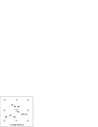
Figure 3: Illustration of the model for the microscopic structure of the body considered in this section. The constituent particles are assumed to be spherical of radius $R$, mass $m_{p}$ and of uniform density. They are separated by an average distance $2D$. The average density of the body is defined to be $\rho_{c}$.

Non-linear effects must therefore be taken into account. Using similar methods to those that were used in section III above, we derive an effective theory that describes the behaviour of the course-grained or macroscopic value of $\phi$ in a body with thin-shell. We will identify the conditions that are required for linear theory averaging to give accurate results and consider what happens when non-linear effects are non-negligible.

In this section, we derive an effective macroscopic theory appropriate for use within bodies that possess a thin-shell and which are made up of small particles, radius $R$ and mass $m_{p}$. These particles are separated by an average distance $2D\gg R$. The average density of the body is $\rho_{c}$. We illustrate this set-up in FIG. 3. A thin-shell, in this sense, means that the average value of $\phi$ inside a sphere of radius $\gtrsim D$, will be approximately constant, $\phi\approx\phi_{c}$, everywhere inside the body apart from in a thin-shell close to the surface of the body. Generally the emergence of a thin-shell is related to a breakdown of linear theory on some level. The conditions for a body to have a thin-shell are given by eqs. (19a-c). The outcome of this section will be to slightly modify these conditions. Precisely, we will find that there is maximal, or critical, value for the average chameleon mass, $m_{c}$. Oddly, this critical, macroscopic chameleon mass depends only on the microscopic properties of the body.

IV.1 Averaging in Linear Theories

We are concerned with finding an effective theory that will give correct value of $\phi_{c}$. We have defined $m_{c}=m_{\phi}(\phi_{c})$. The microscopic field equations for $\phi$, as given by eq. (9), are:

$$-\square\phi=-n\lambda M^{3}\left(\frac{M}{\phi}\right)^{n+1}+\frac{\beta\rho(\vec{x})}{M_{pl}},$$

where the microscopic matter density, $\rho(\vec{x})$, is strongly peaked about the constituent particles of the macroscopic body but negligible in the large spaces between them. Before considering what occurs in a non-linear theory, such as the chameleon theories being studied here, we will review what would occur in the linear case. For the field equation to be linear, the potential must be, at worst, a quadratic in the scalar field $\phi$. With the potentials considered in this paper, a linear theory emerges if $n=0,-1$ or $-2$. To examine why averaging, or coarse graining, is not an issue if field equations are linear, and make reference to what actually occurs in chameleon theories, we shall linearise eq. (9) about $\phi=\phi_{0}$ for some $\phi_{0}$. It is important to note that we are performing this linearisation only for the purpose of showing what occurs in linear theories; we are not claiming that a linearisation, such as this, is actually valid. Defining $\phi=\phi_{0}+\phi_{1}$, and neglecting non-linear terms, we obtain:

$$-\square\phi_{1}=-n\lambda M^{3}\left(\frac{M}{\phi_{0}}\right)^{n+1}+n(n+1)\lambda M^{2}\left(\frac{M}{\phi_{0}}\right)^{n+2}\phi_{1}+\frac{\beta\rho(\vec{x})}{M_{pl}}.$$ (25)

We will write the averaged, or coarse-grained, value of a quantity $Q(\vec{x})$ as $<Q>(\vec{x})$ and define it by:

$$<Q>(\vec{x})=\frac{\int d^{3}y\,Q(\vec{y})\Theta(\vec{x}-\vec{y})}{\int d^{3}y\Theta(\vec{x}-\vec{y})},$$ (26)

where the function $\Theta(\vec{x}-\vec{y})$ defines the coarse graining and the integral is over all space. Different choices of $\Theta$ will result in different coarse-grainings. If we are interested in averaging over a radius of about $D$ around the point $\vec{x}$, then a sensible choice for $\Theta$ would something like:

$$\Theta_{1}(\vec{x}-\vec{y})=e^{-\frac{|\vec{x}-\vec{y}|^{2}}{D^{2}}},$$

or

$$\Theta_{2}(\vec{x}-\vec{y})=H\left(D-|\vec{x}-\vec{y}|\right),$$

where $H(x)$ is the Heaviside function. For the coarse graining process to be well-defined we must require that, whatever choice one makes for $\Theta$, it vanishes sufficiently quickly as $|\vec{x}-\vec{y}|\rightarrow\infty$ that the integrals of eq. (26) converge. This will usually require $\Theta\sim\mathcal{O}(|\vec{x}-\vec{y}|^{-3})$ as $|\vec{x}-\vec{y}|\rightarrow\infty$.

Consider the application of the averaging procedure to the linear field equation given by eq. (25). It follows from the assumed properties of $\Theta$ that $<\square\phi_{1}>=\square<\phi_{1}>$ and so

$$\square<\phi_{1}>=-n\lambda M^{3}\left(\frac{M}{\phi_{0}}\right)^{n+1}+n(n+1)\lambda M^{2}\left(\frac{M}{\phi_{0}}\right)^{n+2}<\phi_{1}>+\frac{\beta<\rho>(\vec{x})}{M_{pl}}.$$

This is the averaged field equation for $\phi_{1}$. It is clear from the above expression, that, although the precise definition of the averaging operator depends on a choice of the function $\Theta$, the averaged field equations are independent of this choice. This independence is a property of linear theories but it is not, in general, seen in non-linear ones. The averaged field equations for a non-linear theory will, generally, depend on ones choice of averaging. In this section, we take our averaging function to be $\Theta_{2}$ as defined above; this is equivalent to averaging by volume in a spherical region of radius $D$. It is also clear that, for a linear theory, the averaged field equation for $\phi_{1}$ is functionally the same as the microscopic equation. This, again, would not be true if non-linear terms where present in the equations; in general

$$<\phi^{n}>\neq<\phi>^{n}$$

unless $n=0$ or $1$ or $\phi$ is a constant.

IV.2 Averaging in Chameleon Theories

Our aim, in this section, is to calculate the correct value of $<\phi>$ and $<m_{\phi}(\phi)>$ inside a body with a thin-shell. We have defined $\phi_{c}=<\phi>$ and $\rho_{c}=<\rho>$. Although these calculations will implicitly depend on our choice of averaging function, our results should also be approximately equal, at least to an order of magnitude, to those that would be found using any other sensible choice of coarse-graining defined over length scales of about $D$ or greater.

If our chameleon theories were linear, we have seen that we would expect $\phi=\phi_{c}^{(lin)}$ where

$$-\square\phi_{c}^{(lin)}=-n\lambda M^{3}\left(\frac{M}{\phi_{c}^{(lin)}}\right)^{n+1}+\frac{\beta\rho_{c}}{M_{pl}},$$

and so, for $\phi_{c}^{(lin)}\approx const$, we have:

$$\phi_{c}^{(lin)}=M\left(\frac{\beta\rho_{c}}{n\lambda M_{pl}M^{3}}\right)^{-1/(n+1)}.$$

In appendix C, we show that, for some values of $R$, $D$ and $m_{p}$, linearised theory will give the correct value of $\phi_{c}$ to a high accuracy i.e. $\phi_{c}\approx\phi_{c}^{(lin)}$. This happens when there either exists a consistent, everywhere valid, linearisation of the field equations or we can construct a pseudo-linear approximation along the same lines as was done in section III.2 . However, for some values of $R$, $D$ and $m_{p}$, we find that non-linear effects are unavoidable. When $R$, $D$ and $m_{p}$ take such values, we will say that we are in the non-linear regime. We find that, just as it did in section III.3 above, the non-linear regime features $\beta$-independent critical behaviour. The details of these calculations can be found in appendix C.

We define:

$$D_{c} = \left(n(n+1)\right)^{\frac{n+1}{n+4}}M^{-1}\left(\frac{3\beta m_{p}}{4\pi M_{pl}|n|}\right)^{\frac{n+2}{n+4}},$$ (27)

$$D_{\ast} = \left(\frac{n(n+1)}{MR}\right)^{\frac{n+1}{3}}M^{-1}\left(\frac{3\beta m_{p}}{4\pi M_{pl}|n|}\right)^{\frac{n+2}{3}},$$

and note that $D_{\ast}/D_{c}=(D_{c}/R)^{(n+1)/3}$. For the linear approximation to be valid we need both $m_{c}D\ll 1$ and $m_{c}^{2}D^{3}/2R\ll 1$. This is equivalent to:

$$D_{c} \ll D\ll D_{\ast},\qquad n<-4$$

$$\max(D_{c},D^{\ast}) \ll D,\qquad n>0.$$

When $n=-4$ we require $D\ll D_{\ast}$ and:

$$(12)^{3/2}\lambda^{1/2}\left(\frac{3\beta m_{p}}{4\pi nM_{pl}}\right)\ll 1.$$

We can see that, for given $m_{p}$ and $R$, it is always possible to find a $D$ such that the linear approximation is valid when $n>0$. However, when $n\leq-4$, it is possible that there will exist no value of $D$ for which the above conditions hold. Whenever the linear approximation holds we have:

$$m_{c}\approx m_{\phi}\left(\phi_{c}^{(lin)}\right).$$

We can construct a pseudo-linear approximation whenever:

$$\left(\frac{D_{c}}{R}\right)^{\frac{n+4}{n+1}}<2|n+1|\left(1-\left(\frac{R}{D}\right)^{\frac{3}{|n+1|}}\right),\qquad n<-4$$ (28a)

$$\frac{D}{D_{c}}>1\quad\mathrm{and}\quad\frac{D_{\ast}}{D}<\left[2(n+1)\left(1-\left(\frac{R}{D}\right)^{\frac{3}{n+1}}\right)\right]^{\frac{n+1}{3}},\qquad n>0$$ (28b)

$$m_{\phi}\left(\phi_{c}^{(lin)}\right)D\ll\left(\frac{243}{2\ln(D/R)}\right)^{1/6},\qquad n=-4.$$ (28c)

When the pseudo-linear approximation holds we again find:

$$m_{c}\approx m_{\phi}\left(\phi_{c}^{(lin)}\right).$$

As the inter-particle separation, $D$, is decreased we will eventually reach a point where eqs. (28a-c) fail to hold. When this occurs it is because non-linear effects have become important inside the individual particles that make up the body. As $D$ decreases still further these particles will eventually develop thin-shells of their own. Non-linear effects become important when:

$$\left(\frac{D_{c}}{R}\right)^{\frac{n+4}{n+1}} > 3|n+1|\left(1-\left(\frac{R}{D}\right)^{\frac{3}{|n+1|}}\right),\qquad n<-4$$ (29a)

$$\frac{D_{\ast}}{D} > \left[3(n+1)\left(1-\left(\frac{R}{D}\right)^{\frac{3}{n+1}}\right)\right]^{\frac{n+1}{3}},\qquad n>0$$ (29b)

$$m_{\phi}\left(\phi_{c}^{(lin)}\right)D \gtrsim \left(\frac{243}{2\ln(D/R)}\right)^{1/6},\qquad n=-4.$$ (29c)

These conditions define the non-linear regime. Between the pseudo-linear, and fully non-linear regimes, there is, of course, some intermediate region, however this has proven too difficult to analyse analytically. We therefore leave the detailed analysis of this intermediate behaviour to a later work. This intermediate region is, however, in some sense small and so we do not believe it to have any great importance with respect to experimental tests of chameleon theories.

When the individual particles develop thin-shells, the $\phi$-field external to the particles will be, by the results of section III, independent of $\beta$. This ensures that the chameleon mass far from the particles is also independent of $\beta$. Therefore, whenever a body falls into the non-linear regime, the average chameleon mass will take a critical value, $m_{c}=m_{c}^{crit}$. This is defined in a similar way to which $(m_{c}R)_{crit}$ was in section III.3, i.e. $m_{c}^{crit}$ is the maximal mass that the chameleon may have when $r\sim{\mathcal{O}}(D)$ such that, when the microscopic field equations are integrated, $(\phi_{c}/\phi)^{n}$ is finite for all $r>R$. This definition implies a relationship between $m_{c}^{crit}$, $R$ and $D$, however it does not depend on either $M$ or $\lambda$. $m_{c}^{crit}$ is also found to depend on $n$; this is because $n$ defines precisely how quickly $(\phi_{c}/\phi)^{n}$ blows up. We derive expressions $m_{c}^{crit}$ in appendix C finding:

$$m_{c}^{crit} \approx \frac{\sqrt{3|n+1|}}{D}\left(\frac{R}{D}\right)^{q(n)/2}S(n),\qquad n\neq-4$$ (30)

$$m_{c}^{crit} = X/D,\qquad n=-4,$$

where $q(n)=\min((n+4)/(n+1),1)$, $S(n)=1$ if $n>0$ and $S(n)=(\gamma(n)/3)^{1/2|n+1|}$ if $n<0$. $X$ is given by:

$$\frac{3\sqrt{3}}{\sqrt{2\ln(D/R)}}\approx X\cosh X-\sinh X.$$

We plot $m_{c}^{crit}D$ vs. $\ln(D/R)$ in figure 4. For an everyday body with density similar to water, we approximate $R$ and $m_{p}$ respectively by the radius and mass of carbon nucleus (say) and find $\ln(D/R)\approx 11$, and so $m_{c}^{crit}\approx 1.4/D$ when $n=-4$. When $n\neq-4$, $m_{c}^{crit}D\ll 1$ follows from $R/D\ll 1$.

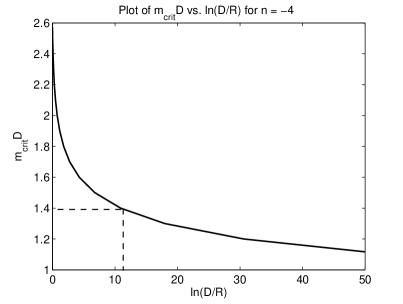
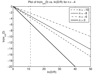
Figure 4: Dependence of the critical chameleon mass on $D/R$. The above plots show how $m_{crit}D$ depends on $\ln(D/R)$ for different values of $n$. The cases $n=-4$ and $n\neq-4$ are qualitatively different and are therefore shown on separate plots. $m_{crit}$ is the maximal mass the chameleon can take inside a thin-shelled body. $2D$ is the average separation of the particles that comprise that body and $R$ is the average radius of the constituent particles. Typically we find that $\ln(D/R)\approx 11$ for bodies with density $\rho\sim 1-10\,{\mathrm{g\,cm}}^{-3}$; $\ln(D/R)=11$ is indicated on the plots. Note that when $n>0$, $m_{crit}D$ is independent of $n$. Also note that in $\phi^{4}$ theory $m_{crit}D\sim\mathcal{O}(1)$ whereas for other value of $n$ it is generically much smaller.

It is interesting to note that, even though $m_{c}^{crit}$ is a macroscopic quantity, it depends entirely on the details of the microscopic structure of the body i.e. $R$ and $D$. By combining the results of this section, we find that the average mass of the chameleon inside a body with thin-shell that is itself made out of particles is given by:

$$m_{c}=\min\left(M\left(\frac{|n|\lambda M_{pl}M^{3}}{\beta\rho_{c}}\right)^{\frac{n+2}{2(n+1)}},m_{c}^{crit}(n,R,D)\right).$$

When evaluating the thin-shell conditions, eqs. (19a-c), it is therefore this value of $m_{c}$ that should be used.

V Force between two bodies

In the previous two sections, we have considered how the chameleon field, $\phi$, behaves both inside and outside an isolated body. In this section we study the form that the chameleon field takes when two bodies are present, and use our results to calculate the resultant $\phi$-mediated force between those bodies. The results of this sections will prove to be especially useful when we come to consider the constraints on chameleon field theories coming from experimental tests of gravity in section VI below.

Chameleon field theories, by their very nature, have highly non-linear field equations. This non-linear nature is especially important when bodies develop thin-shells. As a result of their non-linear structure, one cannot solve the two (or many) body problem by simply super-imposing the fields generated by two (or many) isolated bodies, as one would do for a linear theory.

When the two bodies in question have thin-shells, we shall see that the formula for the $\phi$-force is highly dependent on the magnitude of their separation relative to their respective sizes. We shall firstly consider the case where the separation between the two bodies is small compared the radius of curvature of their surfaces, and secondly look at the force between two distant bodies. Finally we will consider the force between a very small body and a very large body. We will also look at what occurs when one or both of the bodies does not have a thin-shell.

V.1 Force between two nearby bodies

We consider the force between two bodies (hereafter body one and body two) whose surfaces are separated by a distance $d$. Both bodies are assumed to satisfy the thin-shell conditions. The two bodies are taken to be nearby in the sense that: $d\ll R_{1},R_{2}$ where $R_{1}$ and $R_{2}$ are respectively the radii of curvature of the surface of body one and body two. Since $d\ll R_{1},R_{2}$ we can ignore the curvature of the surfaces of bodies to a first approximation. With this simplification we treat the bodies as being infinite, flat slabs and take body one to occupy the region $x<0$, and body two the region $x>d$. We use a subscript $1$ to refer to quantities that are defined for body one: e.g. the density of body one is $\rho_{1}$ and the chameleon mass deep inside body one is $m_{1}$, and a subscript $2$ for quantities relating to body two. Additionally a subscript or superscript $s$ is uses to refer to quantities that are defined on the surfaces of the two bodies e.g. $m_{1}^{s}$ is the chameleon mass of the surface of body one. Subscript $0$ is used two label quantities defined at that point between body one and body two where $d\phi/dx=0$. We assume also that the background chameleon mass, $m_{b}$, obeys $m_{b}d\ll 1$, we discuss later what occurs if this is not the case.

We now consider the $\phi$-mediated force on body one due to body two. With the above definitions, and $\phi$ obeys:

$$\frac{d^{2}\phi}{dx^{2}}=V_{,\phi}(\phi)$$

in $0<x<d$ and

$$\frac{d^{2}\phi}{dx^{2}}=V_{,\phi}(\phi)+\frac{\beta\rho_{1}}{M_{pl}}$$

in $x<0$. Integrating these equations we find:

$$\left(\frac{d\phi}{dx}\right)^{2}=2(V(\phi)-V_{0}),$$ (31)

in $0<x<d$, and in $x<0$ we have:

$$\frac{1}{2}\left(\frac{d\phi}{dx}\right)^{2}=V(\phi)-V_{1}+\frac{\beta\rho_{1}(\phi-\phi_{1})}{M_{pl}}.$$

Matching these expressions at $x=0$ we have:

$$\phi_{1}^{s}-\phi_{1}=\frac{M_{pl}(V_{1}-V_{0})}{\beta\rho_{1}},$$ (32)

If the second body where not present then $V_{0}=0$ and $\phi_{1}^{s}=\bar{\phi}_{1}^{s}$ where:

$$\bar{\phi}_{1}^{s}-\phi_{1}=\frac{M_{pl}V_{1}}{\beta\rho_{1}}.$$

The attractive force per unit area of body one due to body two is therefore:

$$\frac{F_{\phi}}{A}=\frac{\beta\rho_{1}}{M_{pl}}\left|\bar{\phi}_{1}^{s}-\phi_{1}^{s}\right|=V_{0}.$$

This holds for all $V(\phi)$ not just the $\phi^{-n}$ potentials considered in this work. To find $V_{0}$ we integrate eqn. (31) in the region $0<x<d$ and find:

$$\sqrt{2}d=\frac{\sqrt{V_{0}}}{|V_{0,\phi}|}\left(\int^{y_{1}}_{1}\frac{dx}{W(x)\sqrt{x-1}}+\int^{y_{2}}_{1}\frac{dx}{W(x)\sqrt{x-1}}\right),$$ (33)

where $y_{1}=V_{1}^{s}/V_{0}$ and $y_{2}=V_{2}^{s}/V_{0}$ and $W(x=V/V_{0})=V_{\phi}/V_{0,\phi}$. We evaluate the integrals in the above expression in two important limits.

V.1.1 Limit 1: $y_{1}=V_{1}^{s}/V_{0}=1+\delta$

In this limit we assume $V_{1}\approx V_{1}^{s}\approx V_{0}$, this would occur if $V_{1}<V_{2}$ and $d$ is suitably small. In this limit:

$$\int^{y_{1}}_{1}\frac{dx}{W(x)\sqrt{x-1}}=2\int^{\delta^{1/2}}_{0}\frac{dz}{W(1+z^{2})}\approx 2\delta^{1/2}+\mathcal{O}(\delta).$$

We also define $\phi_{1}^{s}-\phi_{1}=\phi_{1}^{s}\epsilon>0$. With this definition equation (32) becomes:

$$\phi_{1}^{s}\epsilon=\frac{M_{pl}\left(V_{1}-V_{1}^{s}\right)}{\beta\rho_{1}}+\frac{M_{pl}V_{0}\delta}{M_{pl}}\approx\phi_{1}^{s}\epsilon+\frac{M_{pl}}{\beta\rho}\left(-\frac{1}{2}\phi_{1}^{s\,2}m_{1}^{2}\epsilon^{2}+V_{0}\delta+\mathcal{O}(\epsilon^{3})\right),$$

thus

$$\phi_{1}^{s}\epsilon\approx\sqrt{\frac{2V_{0}\delta}{m_{1}^{2}}},$$

and

$$V_{0}=V_{1}-\frac{\beta\rho}{M_{pl}}\sqrt{\frac{2V_{1}\delta}{m_{1}^{2}}}+\mathcal{O(\delta)}.$$

V.1.2 Limit 2: $y_{1}=V_{1}^{s}/V_{0}\gg 1$

This limit occurs when either $d$ is suitably large or if $V_{1}\gg V_{2}$. We take $1/y_{1}=\delta\ll 1$. We consider $V\propto\phi^{-n}$ potentials and so $W=x^{1+1/n}$. In this limit we have:

$$\int^{y_{1}}_{1}\frac{dx}{W(x)\sqrt{x-1}}=\int^{1}_{\delta}dz\,z^{\frac{1}{n}-\frac{1}{2}}(1-z)^{-\frac{1}{2}}\approx B\left(\frac{1}{n}+\frac{1}{2},\frac{1}{2}\right)-\left(\frac{2n}{n+2}\right)\delta^{\frac{1}{n}+\frac{1}{2}}+...$$

where $B(\,\cdot\,,\,\cdot\,)$ is the Beta function. To leading order in $\delta$ we have:

$$\phi_{1}^{s}=\phi_{1}+\frac{M_{pl}V_{1}}{\beta\rho_{1}}.$$

We are now in a position to evaluate $V_{0}(d)$ and hence $F_{\phi}/A$. Without loss of generality we take $V_{1}\leq V_{2}$ and consider three limits:

V.1.3 Large separations

If

$$m_{1}d,\,m_{2}d\gg\frac{2\sqrt{2}n}{n+2}\left(\frac{n}{n+1}\right)^{-\frac{n+1}{2}}B\left(\frac{1}{n}+\frac{1}{2},\frac{1}{2}\right).$$

then we have $V_{2}\geq V_{1}\gg V_{0}$ and so:

$$\sqrt{2\lambda}|n|M\left|\frac{M}{\phi_{0}}\right|^{\frac{n}{2}+1}d=2B\left(\frac{1}{n}+\frac{1}{2},\frac{1}{2}\right)+\mathcal{O}\left((V_{0}/V_{1})^{\frac{1}{n}+\frac{1}{2}},(V_{0}/V_{2})^{\frac{1}{n}+\frac{1}{2}}\right).$$

In this limit:

$$\frac{F_{\phi}}{A}=V_{0}=\lambda^{\frac{2}{n+2}}M^{4}\left(\frac{\sqrt{2}B\left(\frac{1}{n}+\frac{1}{2},\frac{1}{2}\right)}{|n|Md}\right)^{\frac{2n}{n+2}}=\lambda^{\frac{2}{n+2}}K_{n}M^{4}(Md)^{\frac{2n}{n+2}},$$

where we have defined

$$K_{n}=\left(\frac{\sqrt{2}B\left(\frac{1}{n}+\frac{1}{2},\frac{1}{2}\right)}{|n|}\right)^{\frac{2n}{n+2}}.$$

V.1.4 Small separations: $m_{2}\approx m_{1}$

If

$$m_{1}d>\left(\frac{n+1}{n}\right)\left(\left(\frac{m_{2}}{m_{1}}\right)^{n/(n+2)}-\left(\frac{m_{1}}{m_{2}}\right)^{n/(n+2)}\right),\quad m_{2}d\ll 1$$

then $V_{2}\approx V_{1}\approx V_{0}$ and:

$$V_{0}\approx V_{1}^{1/2}V_{2}^{1/2}\left[1-\left(\frac{n}{n+1}\right)\frac{V_{0}^{1/2}m_{0}d}{V_{1}^{1/2}+V_{2}^{1/2}}\right]\approx V_{1}^{1/2}V_{2}^{1/2}\left[1-\left(\frac{n}{n+1}\right)\frac{V_{1}^{1/2}m_{1}d}{V_{1}^{1/2}+V_{2}^{1/2}}\right].$$

The force per area is therefore:

$$\frac{F_{\phi}}{A}=V_{1}^{1/2}V_{2}^{1/2}\left[1-\left(\frac{n}{n+1}\right)\frac{V_{0}^{1/2}m_{0}d}{V_{1}^{1/2}+V_{2}^{1/2}}\right]\approx V_{1}^{1/2}V_{2}^{1/2}\left[1-\left(\frac{n}{n+1}\right)\frac{V_{1}^{1/2}m_{1}d}{V_{1}^{1/2}+V_{2}^{1/2}}\right].$$

V.1.5 Small separations: $m_{2}\gg m_{1}$

When $m_{2}\gg m_{1}$ it is generally the case that $V_{2}>V_{1}^{s}\gg V_{0}>V_{1}$. In this case we have:

$$\frac{F_{\phi}}{A}=V_{0}=(n+1)V_{1}\left(1-\left(\frac{m_{1}}{m_{2}}+\left(\frac{n}{n+1}\right)^{\frac{n+2}{2}}\frac{(n+2)m_{1}d}{\sqrt{2n(n+1)}}\right)^{\frac{2}{n+2}}\right).$$

This limit is valid provided that $V_{0}>0$ and $V_{1}^{s}\gg V_{0}$, which requires:

$$\frac{m_{1}}{m_{2}}+\left(\frac{n}{n+1}\right)^{\frac{n+2}{2}}\frac{(n+2)m_{1}d}{\sqrt{2n(n+1)}}\ll 1.$$

If $m_{b}d$ is not $\ll 1$ then the $F_{\phi}/A$ given above are further suppressed by a factor of $\exp(-m_{b}d)$.

V.2 Force between two distant bodies

We shall now consider the force between two bodies, with thin-shells, that are separated by a ‘great distance’, $d$. By ‘great distance’ we mean $d\gg R_{1},\,R_{2}$, where $R_{1}$ and $R_{2}$ are respectively the length scales of body one and body two. Given that $d\gg R_{1},\,R_{2}$, then, to a good approximation, we can consider just the monopole moment of the field emanating from the two bodies, and model each body as a sphere with respective radii $R_{1}$ and $R_{2}$.

We expect that, outside some thin region close to the surface of either body, the pseudo-linear approximation (with the field taking its critical value i.e. $(m_{c}R)\rightarrow(m_{c}R)_{crit}\approx(m_{c}R)_{eff}$) is appropriate to describe the field of either body. In the region where pseudo-linear behaviour is seen, we can safely super-impose the two one body solutions to find the full two body solution.

Close to the surface of body one the mass of the chameleon induced by body one will act to attenuate the perturbation to the chameleon field created by body two. This effect can be quite difficult to model correctly. We can predict the magnitude of the field, however, by noting that the perturbation to $\phi$, induced by body two, near to body one will be

$$\delta\phi_{2}=-\frac{\beta_{eff}^{(2)}{\mathcal{M}}_{2}e^{-m_{b}d}}{4\pi M_{pl}d}.$$

From the results of section III.3, we know that $\beta_{eff}^{(2)}{\mathcal{M}}_{2}/M_{pl}$ only depends on the radius of body two and the theory dependent parameters, $M$, $\lambda$ and $n$; $\beta_{eff}$ is as given in eqs. (24a-c); $m_{b}$ is the mass of the chameleon field in the background i.e. far away from either of the two bodies. ${\mathcal{M}}_{2}$ is the mass of body two.

We define the perturbation to $\phi$ induced by body one near to body one in a similar manner

$$\delta\phi_{1}=-\frac{\beta_{eff}^{(1)}{\mathcal{M}}_{1}e^{-m_{b}d}}{4\pi M_{pl}d}.$$

From eqs. (24a-c) we know that $\delta\phi_{1}$ is independent of $\beta$ and the mass of body one, ${\mathcal{M}}_{1}$. The force on body one due to body two will be proportional to $\nabla\delta\phi_{2}$, however, since this must also be the force on body two due to body one, it must also be proportional to $\nabla\delta\phi_{1}$ evaluated near body two. ¿From this we can see that the force on one body due to the other must, up to a possible ${\mathcal{O}}(1)$ factor, be given by

$$F_{\phi}=\frac{\beta_{eff}^{(1)}{\mathcal{M}}_{1}\beta_{eff}^{(2)}{\mathcal{M}}_{2}(1+m_{b}d)e^{-m_{b}d}}{(4\pi M_{pl})^{2}d^{2}}.$$

The functional dependence of this force on $M$, $n$, $R_{1}$, $R_{2}$ and $\lambda$ depends on whether $n<-4$, $n=-4$ or $n>0$. We consider these three cases separately below. In all cases the force is found to be independent of $\beta$, ${\mathcal{M}}_{1}$ and ${\mathcal{M}}_{2}$.

V.2.1 Case $n<-4$

When $n<-4$, eq. (24a) gives

$$\frac{\beta_{eff}^{(1)}{\mathcal{M}}_{1}}{4\pi M_{pl}}=\left(\frac{\gamma(n)}{|n|}\right)^{\frac{1}{|n+2|}}\left(MR_{1}\right)^{\frac{n+4}{n+2}}.$$

The expression for $\beta_{eff}^{(2)}$ is similar but with $1\rightarrow 2$. The force between two spherical bodies, with respective radii $R_{1}$ and $R_{2}$, separated by a distance $d\gg R_{1},R_{2}$, is therefore given by

$$F_{\phi}=\left(\frac{\gamma(n)}{|n|}\right)^{\frac{2}{|n+2|}}\frac{\left(MR_{1}\right)^{\frac{n+4}{n+2}}\left(MR_{2}\right)^{\frac{n+4}{n+2}}(1+m_{b}d)e^{-m_{b}d}}{d^{2}}.$$ (34)

V.2.2 Case $n>0$

If $n>0$ then $\beta_{eff}^{(1)}$ is given by eq. (24b) to be

$$\frac{\beta_{eff}^{(1)}{\mathcal{M}}_{1}}{4\pi M_{pl}}=MR_{1}\left(\frac{n(n+1)M^{2}}{m_{b}^{2}}\right)^{\frac{1}{n+2}}.$$

Again the expression for $\beta_{eff}^{(2)}$ is similar. The force between two distant bodies is therefore found to be

$$F_{\phi}=\left(\frac{n(n+1)M^{2}}{m_{b}^{2}}\right)^{\frac{2}{n+2}}\frac{M^{2}R_{1}R_{2}(1+m_{b}d)e^{-m_{b}d}}{d^{2}}.$$ (35)

V.2.3 Case $n=-4$

When $n=-4$, $\beta_{eff}^{(1,2)}$ are given by eq. (24c) and they are actually weakly dependent on $r$. Using eq. (24c) we find that

$$F_{\phi}=\frac{(1+m_{b}d)e^{-m_{b}d}}{8\lambda\sqrt{\ln(d/R_{1})\ln(d/R_{2})}d^{2}}.$$ (36)

V.3 Force between a large body and a small body

One subcase that is not included in the above results is the force between a very large body with radius of curvature $R_{1}$, and a very small body with radius of curvature $R_{2}$, that are separated by an intermediate distance $d$ i.e. $R_{2}\gg d\gg R_{1}$. We assume that both bodies have thin-shells. In this case we find a behaviour that is half-way between the two cases described above in sections V.1 and V.2. The magnitude of field produced by the large body will be much greater than that of the small body.

If we ignore the small body and assume that the average mass of the chameleon in the background obeys $m_{b}d\ll 1$, then the field produced by body one is given by eq. (22). Using this equation, we find that

$$\frac{d\phi}{dx}(x=d)\approx\lambda^{\frac{1}{n+2}}\left(\frac{2}{(n+2)^{2}}\right)^{\frac{n}{2(n+2)}}\left(Md\right)^{\frac{n+4}{n+2}}d^{-2}.$$

The effective coupling of body two to this $\phi$-gradient will be $\beta_{eff}$ as it is given by eqs. (24a-c). If $m_{b}d\gtrsim 1$ then this gradient will be, up to an order $\mathcal{O}(1)$ coefficient, attenuated by a factor of $(1+m_{b}d)\exp(-m_{b}d)$. The force between the two bodies is therefore given by

$$F_{\phi} = \left(\frac{\gamma(n)}{|n|}\right)^{\frac{1}{|n+2|}}\left(MR_{2}\right)^{\frac{n+4}{n+2}}\left(\frac{2}{(n+2)^{2}}\right)^{\frac{n}{2(n+2)}}$$ (37a)

$$\left(Md\right)^{\frac{n+4}{n+2}}\frac{(1+m_{b}d)e^{-m_{b}d}}{d^{2}},\qquad n<-4$$

$$F_{\phi} = MR_{2}\left(\frac{n(n+1)M^{2}}{m_{b}^{2}}\right)^{\frac{1}{n+2}}\left(\frac{2}{(n+2)^{2}}\right)^{\frac{n}{2(n+2)}}$$ (37b)

$$\left(Md\right)^{\frac{n+4}{n+2}}\frac{(1+m_{b}d)e^{-m_{b}d}}{d^{2}},\qquad n>0$$

$$F_{\phi} = \frac{1}{2\lambda\sqrt{2\ln(d/R_{2})}}\frac{(1+m_{b}d)e^{-m_{b}d}}{d^{2}},\qquad n=-4.$$ (37c)

As before, $d$ is the distance of separation. These formulae will prove useful when we consider the $\phi$-force between the Earth and a test-mass in laboratory tests for WEP violation in section VI.3.

V.4 Force between bodies without thin-shells

If neither of the two bodies have thin-shells, $\phi$ behaves just like a standard, linear, scalar field with mass $m_{b}$. The force between the two bodies, with masses ${\mathcal{M}}_{1}$ and ${\mathcal{M}}_{2}$, is given by:

$$F_{\phi}=\frac{\beta^{2}{\mathcal{M}}_{1}{\mathcal{M}}_{2}(1+m_{b}d)e^{-m_{b}d}}{4\pi M_{pl}^{2}d^{2}}.$$

As above, $m_{b}$ is the mass of the chameleon in the background. If one of the bodies has a thin-shell, body one say, but the other body does not, then the force is given by

$$F_{\phi}=\frac{\beta_{eff}^{(1)}\beta{\mathcal{M}}_{1}{\mathcal{M}}_{2}(1+m_{b}d)e^{-m_{b}d}}{4\pi d^{2}},$$

whenever $d\gg R_{1}$ where $R_{1}$ is the radius of curvature of body one and $\beta_{eff}^{(1)}$ is as given by eqs. (24). If $d\ll R_{1}$ then

$$F_{\phi}=\lambda^{\frac{1}{n+2}}\left(\frac{2}{(n+2)^{2}}\right)^{\frac{n}{2(n+2)}}\left(Md\right)^{\frac{n+4}{n+2}}\frac{\beta{\mathcal{M}}_{2}(1+m_{b}d)e^{-m_{b}d}}{M_{pl}d^{2}}.$$

As above, $d$ is the distance of separation.

V.5 Summary

In this section we have considered the force that the chameleon field, $\phi$, induces between two bodies, with masses ${\mathcal{M}}_{1}$ and ${\mathcal{M}}_{2}$ and radii $R_{1}$ and $R_{2}$, separated by a distance $d$. The chameleon mass in the far background is taken to be $m_{b}$. When both bodies have thin-shells, we found that, to leading order, the $\phi$-force between them is independent of the matter coupling, $\beta$, provided that $m_{1}d,m_{2}d\gg 1$; $m_{1}$ is the mass that the chameleon has inside body one, and $m_{2}$ is similarly defined with respect to body two. The force between two such bodies is also independent ${\mathcal{M}}_{1}$ and ${\mathcal{M}}_{2}$ but does in general depend on $R_{1}$ and $R_{2}$, as well as on $M$, $n$ and $\lambda$. The main results of this section are summarised below.

Neither body has a thin-shell

$$F_{\phi}=\frac{\beta^{2}{\mathcal{M}}_{1}{\mathcal{M}}_{2}(1+m_{b}d)e^{-m_{b}d}}{4\pi M_{pl}^{2}d^{2}}.$$

Body one has a thin-shell, body two does not

If the two bodies are close together ($m_{1}^{-1}\ll d\ll R_{1}$) then

$$F_{\phi}=\lambda^{\frac{1}{n+2}}\left(\frac{2}{(n+2)^{2}}\right)^{\frac{n}{2(n+2)}}\left(Md\right)^{\frac{n+4}{n+2}}\frac{\beta{\mathcal{M}}_{2}(1+m_{b}d)e^{-m_{b}d}}{M_{pl}d^{2}}.$$

If the bodies are far apart $d\gg R_{1}$ then

$$F_{\phi} = \left(\frac{\gamma(n)}{|n|}\right)^{\frac{1}{|n+2|}}\left(MR_{1}\right)^{\frac{n+4}{n+2}}\frac{\beta{\mathcal{M}}_{2}(1+m_{b}d)e^{-m_{b}d}}{M_{pl}d^{2}},\qquad n<-4,$$

$$F_{\phi} = MR_{1}\left(\frac{n(n+1)M^{2}}{m_{b}^{2}}\right)^{\frac{1}{n+2}}\frac{\beta{\mathcal{M}}_{2}(1+m_{b}d)e^{-m_{b}d}}{M_{pl}d^{2}},\qquad n>0,$$

$$F_{\phi} = (2\lambda\min(d/R,1/m_{b}R))^{-1/2}\frac{\beta{\mathcal{M}}_{2}(1+m_{b}d)e^{-m_{b}d}}{2M_{pl}d^{2}},\qquad n=-4.$$

This force is independent of the mass of body one, and the chameleon’s coupling to it.

Both bodies have thin-shells

If the two bodies of close by and $m_{1}^{-1},m_{2}^{-1}\ll d\ll R_{1},R_{2}$ then the force per unit area is

$$\frac{F_{\phi}}{A}\approx\lambda^{\frac{2}{2+n}}M^{4}\left[\frac{\sqrt{2}B\left(\frac{1}{2},\frac{1}{2}+\frac{1}{n}\right)}{|n|Md}\right]^{\frac{2n}{n+2}}.$$

Different formulae for $F_{\phi}/A$ apply if either $m_{1}d<1$ or $m_{2}d<1$, these are given at the end of section V.1 above.

$$F_{\phi} = \left(\frac{\gamma(n)}{|n|}\right)^{\frac{2}{|n+2|}}\frac{\left(MR_{1}\right)^{\frac{n+4}{n+2}}\left(MR_{2}\right)^{\frac{n+4}{n+2}}(1+m_{b}d)e^{-m_{b}d}}{d^{2}},\quad n<-4$$

$$F_{\phi} = \left(\frac{n(n+1)M^{2}}{m_{b}^{2}}\right)^{\frac{2}{n+2}}\frac{M^{2}R_{1}R_{2}(1+m_{b}d)e^{-m_{b}d}}{d^{2}},\quad n>0$$

$$F_{\phi} = \frac{(1+m_{b}d)e^{-m_{b}d}}{8\lambda\sqrt{\ln(d/R_{1})\ln(d/R_{2})}d^{2}},\quad n=-4,$$

where $\gamma(n)$ is given in table 1. If body one is much larger than body two and they are at an intermediate separation: $R_{2},m_{1}^{-1}\gg d\gg R_{1}$ then

$$F_{\phi} = \left(\frac{\gamma(n)}{|n|}\right)^{\frac{1}{|n+2|}}\left(MR_{2}\right)^{\frac{n+4}{n+2}}\left(\frac{2}{(n+2)^{2}}\right)^{\frac{n}{2(n+2)}}$$

$$\left(Md\right)^{\frac{n+4}{n+2}}\frac{(1+m_{b}d)e^{-m_{b}d}}{d^{2}},\qquad n<-4$$

$$F_{\phi} = MR_{2}\left(\frac{n(n+1)M^{2}}{m_{b}^{2}}\right)^{\frac{1}{n+2}}\left(\frac{2}{(n+2)^{2}}\right)^{\frac{n}{2(n+2)}}$$

$$\left(Md\right)^{\frac{n+4}{n+2}}\frac{(1+m_{b}d)e^{-m_{b}d}}{d^{2}},\qquad n>0$$

$$F_{\phi} = \frac{1}{2\lambda\sqrt{2\ln(d/R_{2})}}\frac{(1+m_{b}d)e^{-m_{b}d}}{d^{2}},\qquad n=-4.$$

VI Laboratory Constraints

The best bounds on corrections to General Relativity come from laboratory experiments such as the Eöt-Wash experiment, EotWash and Lunar Laser Ranging tests for WEP violations, LLR ; LLR1 . At very small distances $d\lesssim 10\mu m$, the best bounds on the strength of any fifth force come from measurements of the Casimir force.

In this section we will consider, to what extent, the results of these tests constrain the class of chameleon field theories considered here. We will find the rather startling result that $\beta\gg 1$ is not ruled out for chameleon theories.

One of original reasons for studying chameleon theories with $n>0$ potentials, chama , was that the condition for an object to have a thin-shell, eq. (19b), was found to depend on the background density of matter. It is clear from eq. (19b), that the smaller $\rho_{b}$ is, the larger $m_{c}R$ must be for a body to have a thin-shell. This property lead the authors of ref. chama to conclude that the thin-shell suppression of the fifth-force associated with $\phi$ would be weaker for tests performed in the low density vacuum of space $\rho_{b}\sim 10^{-25}\,{\mathrm{g\,cm}}^{-3}$, than it is in the relatively high density laboratory vacuum $\rho_{b}\sim 10^{-17}\,{\mathrm{g\,cm}}^{-3}$. As a result, it is possible that, if the same experimental searches for WEP violation, which were performed in the laboratory in WEP ; WEP1 ; WEP2 ; willbook ; willbook1 , were to be repeated in space, they would find equivalence principle violation at a level greater than that already ruled out by the laboratory-based tests. It is important to note that this is very much a property of $n>0$ theories. It is clear from eqs. (19a) and (19c) that, when $n\leq-4$, the thin-shell condition, for a body of density $\rho_{c}$, is only very weakly dependent on the background density of matter when $\rho_{b}\ll\rho_{c}$. As a result, space-based searches for WEP violation will not detect any violation at a level that is already ruled by lab-based tests for $n\leq-4$ theories. Planned space-based tests such as STEP STEP , SEE SEE , GG GG and MICROSCOPE MICRO promise a much greater precisions than their lab-based counterparts. MICROSCOPE is due to be launched in 2007. This improved precision will, in all cases, provide us with better bounds on chameleon theories.

VI.1 Eöt-Wash experiment

The University of Washington’s Eöt-Wash experiment, EotWash ; Eotnew , is designed to search for deviations from the $1/r^{2}$ drop-off gravity predicted by General Relativity. The experiment uses a rotating torsion balance to measure the torque on a pendulum. The torque on the pendulum is induced by an attractor which rotates with a frequency $\omega$. The attractor has 42 equally spaced holes, or ‘missing masses’, bored into it. As a result, any torque on the pendulum, which is produced by the attractor, will have a characteristic frequency which is some integer multiple of $21\omega$. This characteristic frequency allows any torque due to background forces to be identified in a straightforward manner. The torsion balance is configured so as to factor out any background forces. The attractor is manufactured so that, if gravity drops off as $1/r^{2}$, the torque on the pendulum vanishes.

The experiment has been run with different separations between the pendulum and attractor. The Eot-Wash group recently announced some new results which go a long way towards better constraining the parameter space of chameleon theory, Eotnew . The experiment has been run for separations, $55\mu m\leq d\leq 9.53mm$. Both the attractor and the pendulum are made out of molybdenum with a density of about $\rho_{Mb}\sim 10\,{\mathrm{g\,cm}}^{-3}$ and are $0.997\,{\mathrm{mm}}$ thick. Electrostatic forces are shielded by placing a $10\,\mu{\mathrm{m}}$ thick, uniform BeCu sheet between the attractor and pendulum. The density of this sheet is $\rho_{BeCu}\sim 8.4\,{\mathrm{g\,cm}}^{-3}$. The rôle played by this sheet is crucial when testing for chameleon fields. If $\beta$ is large enough, the sheet will itself develop a thin-shell. When this occurs the effect of the sheet is not only to shield electrostatic forces, but also to block any chameleon force originating from the attractor.

The force per unit area between the attractor and pendulum plates due to a scalar field with matter coupling $\beta$ and constant mass $m$, where $1/m\ll 0.997mm$ is:

$$|\frac{F}{A}|=\frac{\alpha e^{-md}2\pi G\rho_{Mb}^{2}}{m^{2}}$$

where $\alpha=\beta^{2}/4\pi$ and $d$ is the separation of the two plates. The strongest bound on $\alpha$ coming from the Eot-Wash experiment is $\alpha<2.5\times 10^{-3}$ for $1/m=0.4\,--\,0.8mm$.

Depending on the values of $\beta$, $M$ and $\lambda$ there are three possible situations:

• The pendulum and the attractor have thin-shells, but the BeCu sheet does not

• The pendulum, the attractor and the BeCu sheet all have thin-shells.

• Neither the test masses nor the BeCu sheet have thin-shells.

In the first case the $\phi$-mediated force per unit area in a perfect vacuum is given by one of the equations derived in section V.1 (depending on the separation $d$). In reality the vacuum used in these experiments is not perfect actually has a pressure of $10^{-6}\,\mathrm{Torr}$ which means that the chameleon mass in the background, $m_{b}$, is non-zero and so $F_{\phi}/A$ is suppressed by a factor of $\exp(-m_{b}d)$. Fortunately however $m_{b}d\ll 1$ for all but the largest $\beta$. A further, and far more important, suppression occurs when the BeCu sheet has a thin-shell. If $m_{BeCu}$ is the chameleon mass inside the BeCu sheet and $d_{BeCu}$ the sheet’s thickness, the existence of a thin-shell in the electromagnetic shield causes the chameleon mediated force between the pendulum and attractor to be suppressed by a further factor of $\exp(-m_{BeCu}d_{BeCu})$. The thin-shell condition for the BeCu sheet implies that $m_{BeCu}d_{BeCu}\gg 1$, and so this suppression all but removes any detectable chameleon induced torque on the pendulum due to the attractor. The BeCu sheet will itself produce a force on pendulum but, since the sheet is uniform, this force will result in no detectable torque. If $M$ and $\lambda$ take natural values the electromagnetic sheet develops a thin-shell for $\beta\gtrsim 10^{4}$: as a result of this the Eot-Wash experiment can only very weakly constrain large $\beta$ theories.

If neither the pendulum or the attractor have thin-shells then we must have $m_{b}d\ll 1$ and the chameleon force is just $\beta^{2}/4\pi$ times the gravitational one. Since this force drops of as $1/r^{2}$ it will be undetectable from the point of view this experiment. In this case, however, $\beta$ is constrained by other experiments such as those that search for WEP violation LLR ; LLR1 ; WEP ; WEP1 ; WEP2 or those that look for Yukawa forces with larger ranges Irvine .

Given all of the considerations mentioned above, we used the formulae given in section V.1 to evaluate the latest Eöt-Wash constraints on the parameter space of chameleon theories. Our results are shown in FIG 5.

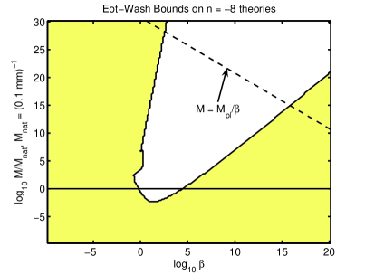
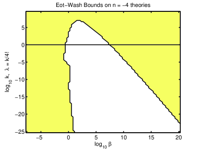
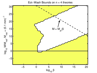
Figure 5: [Colour Online] Constraints on chameleon theories coming from the Eöt-Wash bounds on deviations from Newton’s law. The shaded area shows the regions of parameter space that are allowed by the current data. The solid black lines indicate the cases where $M$ and $\lambda$ take ‘natural values’. The dotted-black line indicates when $M=M_{\phi}:=M_{pl}/\beta$ i.e. when the mass scale of the potential is the same as that of the matter coupling. Other $n<-4$ theories are similar to the $n=-8$ case, whilst the $n=4$ plot is typical of what is allowed for $n>0$ theories. The amount of allowed parameter space increases with $|n|$.

In these plots the shaded region is allowed by the current bounds.

When $\beta$ is small, the chameleon mechanism present in these theories becomes very weak, and from the point of view of the Eöt-Wash experiment, $\phi$ behaves like a normal (non-chameleon) scalar field. When $\beta\gg 1$, the $\phi$-force is independent of the coupling of the chameleon to attractor or the pendulum, but does depend on the mass of the chameleon in the BeCu sheet, $m_{BeCu}$. The larger $m_{BeCu}$ is, the weaker the Eöt-Wash constraint becomes. Larger $\beta$ implies a larger $m_{BeCu}$, and this is why the allowed region of parameter space increases as $\beta$ grows to be very large.

When $n=-4$, we can see that a natural value of $\lambda$ is ruled out for $10^{-1}\lesssim\beta\lesssim 10^{4}$, but is permissible for $\beta\gtrsim 10^{4}$. This is entirely due to the that BeCu sheet has a thin-shell, in $n=-4$ theories with $\lambda=1/4!$, whenever $\beta\gtrsim 10^{4}$.

It is important to stress that, despite the fact that the Eöt-Wash experiment is currently unable to detect $\beta\gg 1$, this is not due to a lack of precision. One pleasant feature, of the $\beta$-independence of the $\phi$-force, is that if you can detect, or rule out, such a force for one value of $\beta\gg 1$, then you will be able to detect it, or rule out, all such $\beta\gg 1$ theories. If design of the experiment can be altered so that electrostatic forces are compensated without using a thin-sheet then the experimental precision already exists to detect, or rule out, almost all $\beta\gg 1$, $\phi^{4}$ theories with $\lambda\approx 1/4!$.

In conclusion, an experiment, along the same lines of the Eöt-Wash test, could detect, or rule out, the existence of sub-Planckian, chameleon fields with natural values of $M$ and $\lambda$ in the near future, provided it is designed to do so.

VI.2 Casimir force experiments

Short distance tests of gravity fail to constrain strongly coupled chameleon theories as a result of their use of a thin metallic sheet to shield electrostatic forces. However, experiments designed to detect the Casimir force between two objects, control electrostatic effects by inducing an electrostatic potential difference between the two test bodies. By varying this potential difference and measuring the force between the test masses, it is possible to factor out electrostatic effects. As a result, Casimir force experiments provide an excellent way in which to bound chameleon fields where the scalar field is strongly coupled to matter.

Casimir force experiments measure the force per unit area between two test masses separated by a distance $d$. It is generally the case that $d$ is small compared to the curvature of the surface of the two bodies and so the test masses can be modeled, to a good approximation, as flat plates.

In section V.1 we evaluated the force per unit area between two flat, thin-shelled slabs with densities $\rho_{1}$ and $\rho_{2}$. The Casimir force is between two such plates is:

$$\frac{F_{Cas}}{A}=\frac{\pi^{2}}{240d^{4}}.$$

Whilst a number of experimental measurement of the Casimir force between two plates have been made, the most accurate measurements of the Casimir force have been made using one sphere and one slab as the test bodies. The sphere is manufactured so that its radius of curvature, $R$, is much larger than the minimal distance of separation $d$. In this case the total Casimir force between the test masses is:

$$F_{Cas}=2\pi R\left(\frac{1}{3}\frac{\pi^{2}}{240}\frac{1}{d^{3}}\right)=3.35\left(\frac{R}{d^{3}}\frac{(\mu m)^{3}}{cm}\right)\mu\mathrm{dyn}.$$

In all cases, apart from when $n=-4$ and $m_{1}d,m_{2}d\gg 1$, the chameleon force per area grows more slowly than $d^{-4}$ as $d\rightarrow 0$. When $n=-4$ and $m_{1}d,m_{2}d\gg 1$ we have $F_{\phi}/A\propto d^{-4}$. It follows that the larger the separation, $d$, used, the better Casimir force searches constrain chameleon theories. Additionally, these tests provide the best bounds when the test masses do have thin-shells as this results in a strongly $d$ dependent chameleon force. Large test masses are therefore preferable to small ones.

Note that if the background chameleon mass is large enough that $m_{b}d\gtrsim 1$ then $F_{\phi}$ is suppressed by a factor of $\exp(-m_{b}d)$. The smaller the background density, $\rho_{b}$, is, the smaller $m_{b}$ become. Since small $m_{b}$ is clearly preferably, the best bounds come from experiments that use the lowest pressure laboratory vacuum.

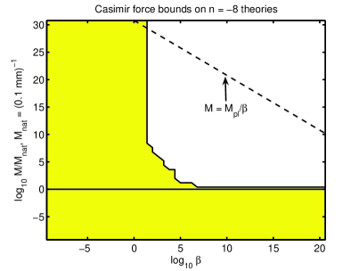
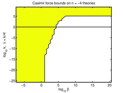
Figure 6: [Colour Online] Constraints on chameleon theories coming from experimental searches for the Casimir force. The shaded area shows the regions of parameter space that are allowed by the current data. The solid black lines indicate the cases where $M$ and $\lambda$ take ‘natural values’. The dotted-black line indicates when $M=M_{\phi}:=M_{pl}/\beta$ i.e. when the mass scale of the potential is the same as that of the matter coupling. Other $n<-4$ theories are similar to the $n=-8$ case, whilst the $n=4$ plot is typical of what is allowed for $n>0$ theories. The amount of allowed parameter space increases with $|n|$ i.e. as the potential becomes steeper.

In Lamcas , Lamoreaux reported the measurement of the Casimir force using a torsion balance between a sphere, with radius of curvature $12.5\mathrm{cm}\pm 0.3\mathrm{cm}$ and diameter of $4\mathrm{cm}$, and a flat plate. The plate was $0.5\mathrm{cm}$ thick and $2.54\mathrm{cm}$ in diameter. The apparatus of placed in a vacuum with a pressure of $10^{-4}\mathrm{mbar}$. Distances of separation of $6-60\mu\mathrm{m}$ we used and in the region $d\approx 7-10\mu\mathrm{m}$ it was found that:

$$|F^{measured}-F_{Cas}^{theory}|\lesssim 1\mu\,\mathrm{dyn}.$$

Another measurement, this time using a microelectromechanical torsional oscillator, was performed by Decca et al. and reported in Decca . In this experiment, the sphere was much smaller than that used by Lamoreaux, being on $296\pm 2\mu\mathrm{m}$ in radius; the plate was made of $3.5\mu\mathrm{m}$ thick, $500\times 500\mu\mathrm{m}^{2}$ polysilicon. The smallness of these test masses means that they will only have thin-shells when $\beta$ is very large. In the region $d\approx 400n\mathrm{m}-1200n\mathrm{m}$, $|F^{measured}-F_{Cas}^{theory}|\lesssim 7.5\times 10^{-2}\mu\mathrm{dyn}$. We show how these experiments constrain the parameter space of $\phi^{-n}$ chameleon theories in FIG 6. Other Casimir force tests (e.g. othercas ) are less suited to constraining chameleon theories such as those considered here. As in the previous plots, the shaded area is allowed, the solid black line is $M\sim(\rho_{\Lambda})^{1/4}$ or $\lambda=1/4!$, and the dotted black line is $M=M_{pl}/\beta$. We note that Casimir force experiments provide very tight bounds on $\lambda$ and $M$ when $\beta\gg 1$. A natural value of $\lambda$ when $n=-4$ is ruled out for all $\beta\geq 10^{4}$. When this is combined with the latest Eöt-Wash data we can rule out $\lambda=1/4!$ for all $\beta>1$. For other $n$, we see that we cannot have $M$ much larger than its ‘natural’ value $(\rho_{\Lambda})^{1/4}$ for large $\beta$. If the bounds on extra forces at $d\sim 1-10\mu m$ can be tighten by roughly an order of magnitude then a natural value of $M$ can be ruled out for all large $\beta$. Casimir force tests provided by far the best bounds on $M$ and $\lambda$ for large $\beta$. We note that $n=-4$ theories are the most tightly constrained by Casimir force experiments, this is not surprising since $F_{\phi}/F_{Cas}\sim const$ and is $>1$ in the region when $m_{1}d,m_{2}d\gg 1$ in this model, whereas in all the other theories $F_{\phi}/F_{Cas}$ decreases as $d$ is made smaller.

More generally, the steeper the potential in a given theory is, the more slowly $F_{\phi}/A$ increases as $d\rightarrow 0$ and, as a result, the weaker Casimir force bounds on the theories parameter space are.

VI.3 WEP violation experiments

The weak equivalence principle (WEP) is the statement that the (effective) gravitational and inertial mass of a body are equal. If it is violated then the either the strength of gravitational force on a body depends on its composition, or there is a composition dependent ‘fifth-force’. Since we believe that gravity is geometric in nature, most commentators, ourselves included, would tend to interpret any detection of a violation of WEP in terms of the latter option. The existence of light scalar fields that couple to matter usually results in WEP violations. As we mentioned in the introduction to this thesis, the experimental bounds on WEP violation are exceeding strong, LLR ; LLR1 ; willbook ; willbook1 ; fischbach ; WEP ; WEP1 ; WEP2 , and, at present, they represent the strongest bounds on the parameters of, non-chameleon, scalar-tensor theories such as Brans-Dicke theory, uzan ; BD . A number of planned satellite missions promise to increase the precision to which we can detect violations of WEP by between 2 to 5 orders of magnitude MICRO ; SEE ; STEP ; GG . The precision that is achievable in laboratory based tests also continues to increase at a steady rate.

Experiments that search for violations of the weak equivalence principle generally fall into two categories: laboratory based experiments, which often employ a modified torsion balance, WEP ; WEP1 ; WEP2 , and solar system tests such as lunar laser ranging (LLR) LLR ; LLR1 .

The laboratory based searches use a modified version of the Eöt-Wash experiment mentioned above. In these experiments the test masses are manufactured to have different compositions. The aim is then to detect, and measure, any difference in the acceleration of test-masses towards an attractor, which is usually the Earth, the Sun or the Moon. In some versions of the experiment a laboratory body is used as the attractor.

If the test masses have thin-shells then the $\phi$-force pulling them towards the Earth is given by equations (37a-c). The chameleon force towards the Moon or Sun is given by eqs. (34)-(36). If the attractor is a laboratory body then, depending on the separations used, the force is given by either eqs. (34)-(36) or by eq. (V.1).

We label the mass and radius of the attractor by ${\mathcal{M}}_{3}$ and $R_{3}$ respectively, and take the mass and radius (or size) of the two test-masses to be given by $\{{\mathcal{M}}_{1},\,R_{1}\}$ and $\{{\mathcal{M}}_{2},\,R_{2}\}$. We define $\alpha_{13}$ to be the relative strength, compared to gravity, of $\phi$-force between the attractor (body three) and the first of the test masses (body one). $\alpha_{23}$ is defined similarly as a measure of the $\phi$-force between body two and body three. The difference between the acceleration of the two test masses towards the attractor is quantified by the Eötvos parameter, $\eta$, where

$$\eta=\frac{2|\alpha_{13}-\alpha_{23}|}{|2+\alpha_{13}+\alpha_{23}|}\approx|\alpha_{13}-\alpha_{23}|.$$

When the test-bodies have thin-shells, we found, in section V, that the $\phi$-force is independent of the masses of the test-bodies, the mass of the attractor and the coupling of the test-masses and attractor to the chameleon. The only property of the attractor and test bodies, which the $\phi$-force does depend on, is their respective radii. Since the gravitational force between the test-masses and the attractor does depend on the masses of the bodies, it follows that $\alpha_{13}$ only depends on ${\mathcal{M}}_{1}$, ${\mathcal{M}}_{3}$, $R_{1}$, $R_{3}$, $M$ (or $\lambda$), $m_{b}$ and $n$, where $m_{b}$ is the chameleon mass in the background. It does not depend on the chameleon’s coupling to the test-mass, $\beta$. The situation with $\alpha_{23}$ is very similar.

Since the $\phi$-force is independent of the coupling, $\beta$, any microscopic composition dependence in $\beta$ will be hidden on macroscopic length scales. The only ‘composition’ dependence in $\alpha_{13}$ is through the masses of the bodies and their dimensions ($R_{1}$ and $R_{3}$).

Taking the third body to be the Earth, the Sun or the Moon, experimental searches for WEP violations have, to date, found that $\eta\lesssim 10^{-13}$ WEP ; WEP1 ; WEP2 . Future satellite tests promise to be able to detect violations of WEP at between the $10^{-15}$, MICRO , and the $10^{-18}$ level, STEP . It also is claimed that future laboratory tests will be able to see $\eta\sim 10^{-15}$, however, whilst the precision to detect at such a level is achievable, there are a number of systematic effects that need to be compensated for, before an accurate measurement can be made.

In most of these searches, although the composition of the test-masses is different, they are manufactured to have the same mass (${\mathcal{M}}_{1}={\mathcal{M}}_{2}$) and the same size ($R_{1}=R_{2}$). Therefore, if the test-masses have thin-shells, we will have $\alpha_{13}=\alpha_{23}$ and so $\eta=0$ identically. As a result, a chameleon field will produce no detectable WEP violation in these experiments. The only implicit dependence of this result on $\beta$ is that, the larger the coupling is, the more likely it is that the test-masses will satisfy the thin-shells conditions.

If one wishes to detect the chameleon using WEP violations searches, then one must either ensure that test-masses do not satisfy the thin-shell conditions, or that they have different masses and/or dimensions.

We have just argued that all of the chameleon theories considered here will automatically satisfy all laboratory bounds on WEP violation, provided the test-masses have thin-shells. This occurs entirely as a result of the design of those experiments.

Let us consider then a putative experiment, which could be conducted, that would, in principle, be able to detect the chameleon through a violation of WEP. In this experiment the test masses are of different densities ($\rho_{1}$ and $\rho_{2}$) but of the same mass, ${\mathcal{M}}_{test}$. Crucially the radii (size) of the two bodies are taken to be different: $R_{1}$ and $R_{2}$. We now calculate the Eötvos parameter, $\eta$, taking the attractor to be either the Earth, the Sun or the Moon.

VI.3.1 Attractor is the Earth

If the attractor is the Earth then we obtain

$$\eta = \left(\frac{M_{pl}^{2}(1+m_{b}d)e^{-m_{b}d}}{{\mathcal{M}}_{E}{\mathcal{M}}_{test}}\right)\left(\frac{3}{|n|}\right)^{\frac{1}{|n+2|}}\left|\left(MR_{1}\right)^{\frac{n+4}{n+2}}-\left(MR_{2}\right)^{\frac{n+4}{n+2}}\right|$$

$$\left(\frac{2}{(n+2)^{2}}\right)^{\frac{n}{2(n+2)}}\left(Md\right)^{\frac{n+4}{n+2}},\qquad n<-4,$$

$$\eta = \left(\frac{M_{pl}^{2}(1+m_{b}d)e^{-m_{b}d}}{{\mathcal{M}}_{E}{\mathcal{M}}_{test}}\right)\left(\frac{n(n+1)M^{2}}{m_{b}^{2}}\right)^{\frac{1}{n+2}}\left|M(R_{1}-R_{2})\right|$$

$$\left(\frac{2}{(n+2)^{2}}\right)^{\frac{n}{2(n+2)}}\left(Md\right)^{\frac{n+4}{n+2}},\qquad n>0,$$

$$\eta = \left(\frac{M_{pl}^{2}(1+m_{b}d)e^{-m_{b}d}}{4\sqrt{2}\lambda{\mathcal{M}}_{E}{\mathcal{M}}_{test}}\right)\left|\frac{1}{\sqrt{\ln(d/R_{1})}}-\frac{1}{\ln(d/R_{2})}\right|,\qquad n=-4,$$

where $m_{b}$ is the mass of the chameleon in the background region between the test masses and the surface of the Earth; $d$ is the distance between the test masses and the surface of the Earth. ${\mathcal{M}}_{Earth}$ is the mass of the Earth, and $R_{Earth}$ its radius.

Current experimental precision bounds $\eta\lesssim 10^{-13}$. We shall assume that our putative experiment, if conducted, would find $\eta\lesssim 10^{-13}$. However, even if this is the case, we are still only able to recover very weak bounds on $\{\beta,M,\lambda\}$. The bounds on $\beta$ are especially weak due to the $\beta$-independence of the $\phi$-force whenever the test-bodies have thin-shells. The only real bound on $\beta$ comes out of requirement that it be large enough for the test-masses to have thin-shells.

For definiteness, we take the test-masses to be spherical, with a mass of ${\mathcal{M}}_{test}=10\,g$. We assume that one of them is made entirely of copper and the other from aluminum. If the test-masses have thin-shells then, even if $m_{b}d\ll 1$, finding $\eta<10^{-13}$ would, when $n=-4$, only limit

$$\lambda\gtrsim 10^{-30}.$$

For theories with $n<-4$, $\eta<10^{-13}$ is easily satisfied provided that: $M<10^{10}\,{\mathrm{mm}}^{-1}$. When $n>0$, the resultant bound is on a combination of $M$ and $m_{b}^{2}$. The WEP bounds on the parameter space of $n>0$ theories are generally stronger than those for other $n$. We plot the effect of these bounds on the parameter space of our chameleon theories in FIG 7.

VI.3.2 Attractor is the Sun or the Moon

Constraints on chameleon theories can also be found by considering the differential acceleration of the test masses towards the Moon or the Sun, rather than towards the Earth. The analysis for both of these scenarios proceeds along the much same lines. Since, for the reasons we explain below, the lunar bound will be by far the stronger, we will only explicitly consider the case where the third body is the Moon. In this case, the force between the test mass and the Moon is given by equations (34), (35) and (36) for $n<-4$, $n>0$ and $n=-4$ respectively.

We define $m_{b}$ to be the average chameleon mass in the region between the Earth and the Moon, and $m_{atm}$ to be the mass of the chameleon in the Earth’s atmosphere; $m_{lab}$ is the background mass of the chameleon in the laboratory. $R_{a}$ is the thickness of the Earth’s atmosphere. $d$ is the distance of separation between the laboratory apparatus and the Moon. Evaluating $\eta$ we find:

$$\eta = \left(\frac{M_{pl}^{2}(1+m_{b}d)e^{-m_{b}d-m_{a}R_{a}}}{{\mathcal{M}}_{Moon}{\mathcal{M}}_{test}}\right)\left(\frac{3}{|n|}\right)^{\frac{2}{|n+2|}}$$

$$\left(MR_{Moon}\right)^{\frac{n+4}{n+2}}\left|\left(MR_{1}\right)^{\frac{n+4}{n+2}}-\left(MR_{2}\right)^{\frac{n+4}{n+2}}\right|,\qquad n<-4$$

$$\eta = \left(\frac{M_{pl}^{2}(1+m_{b}d)e^{-m_{b}d-m_{a}R_{a}}}{{\mathcal{M}}_{Moon}{\mathcal{M}}_{test}}\right)$$

$$\left(\frac{n(n+1)M^{2}}{m_{b}m_{lab}}\right)^{\frac{2}{n+2}}MR_{Moon}|M(R_{1}-R_{2})|,\qquad n>0,$$

$$\eta = \left(\frac{M_{pl}^{2}(1+m_{b}d)e^{-m_{b}d-m_{a}R_{a}}}{{8\lambda\mathcal{M}}_{Moon}{\mathcal{M}}_{test}}\right)$$ (41)

$$\left|\frac{1}{\sqrt{\ln(d/R_{1})\ln(d/R_{Moon})}}-\frac{1}{\sqrt{\ln(d/R_{2})\ln(d/R_{Moon})}}\right|,$$

where ${\mathcal{M}}_{Moon}$ is the mass of the Moon and $R_{Moon}$ its radius. If the Sun is used as the attractor then $\eta$ is given by a similar set of equations to those shown above only with ${\mathcal{M}}_{Moon}\rightarrow{\mathcal{M}}_{Sun}$ and $R_{Moon}\rightarrow R_{Sun}$. $M_{Sun}$ and $R_{Sun}$ are respectively the mass and the radius of the Sun. If the attractor is taken to have fixed density, then we can see that $\eta$ dies off at least as quickly as $1/R^{2}$, where $R$ is the radius of the attractor. It follows that the predicted value $\eta$, induced by chameleon, is always smaller when the Sun is used as the attractor than when the Moon is. This is because $R_{Sun}\gg R_{Moon}$.

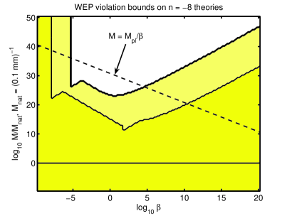
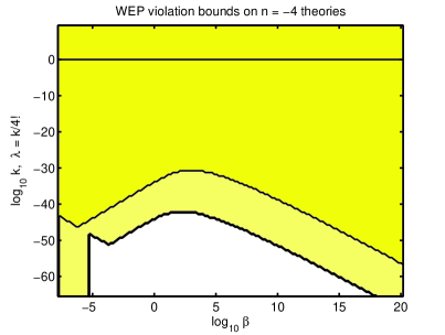
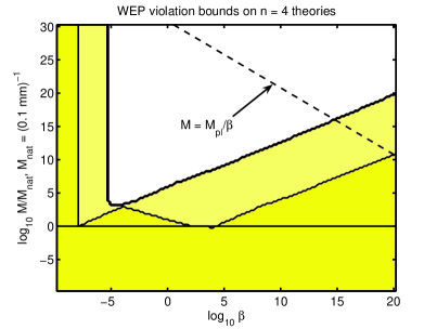
Figure 7: [Colour Online] Constraints on chameleon theories coming from WEP violation searches. The whole of shaded area shows the regions of parameter space that are allowed by the current data. Future space-based tests could detect the more lightly shaded region. The solid black lines indicate the cases where $M$ and $\lambda$ take ‘natural values’. The dotted-black line indicates when $M=M_{\phi}:=M_{pl}/\beta$ i.e. when the mass scale of the potential is the same as that of the matter coupling. Other $n<-4$ theories are similar to the $n=-8$ case, whilst the $n=4$ plot is typical of what is allowed for $n>0$ theories. The amount of allowed parameter space increases with $|n|$.

The predicted values of $\eta$ have a similar dependence on the radii of the test-masses i.e. dying off at least as quickly as $1/R^{2}$. The corollary of this result is that if we are unable to detect $\phi$ in lab-based, micro-gravity experiments where the radii of the test-masses and the attractor are both of the order of $10\,{\mathrm{cm}}$, or smaller, then the $\phi$-force between larger (say human-sized) objects would also be undetectably small. For this reason, in the context of chameleon theories, measurements of the differential acceleration of the Earth and Moon towards the Sun, e.g. lunar laser ranging LLR ; LLR1 , are not competitive with the bounds on WEP violation found in laboratory-based searches.

VI.3.3 Summary

We show how bounding the Eötvos parameter by $\eta<10^{-13}$, with the attracting body being either the Moon or the Earth, constrains chameleon theories in FIG. 7. As with the Eöt-Wash plots: the whole of the shaded area is currently allowed, whilst the more lightly shaded area is that which could be detected by proposed space-based tests of gravity such as SEE, STEP, GG and MICROSCOPE. It is claimed, STEP ; SEE ; MICRO ; GG , that these experiments will be able to detect $\eta$ down to $10^{-18}$. This improved precision is responsible for most of the increased ability of spaced based tests to detect a chameleon field. When $n>0$, the thin-sell condition is stronger in the low density background of space than it is in the relatively higher density background of the laboratory; this effect accounts for some of extra ability that future space-based experiments have to detect the chameleon. We note that WEP violation searches only have any real hope of detecting the chameleon field, if $M$ take a ‘natural’ value i.e. $M\sim(0.1{\mathrm{mm}})^{-1}$, in $n>0$ theories.

VI.4 Discussion

In FIG. 7, we plot how all of the bounds on WEP violation mentioned in refs. WEP ; WEP1 ; WEP2 ; LLR ; LLR1 , as well as the putative bound resulting from the modified WEP violation test we considered above, constrain the parameter space of our chameleon theories. The Eöt-Wash bounds are shown in FIG. 5, and the Casimir bounds in FIG. 6 These Eöt-Wash, Casimir and WEP violation bounds are also included in the plots of section IX.

It is important to note that, the larger $\beta$ is, the stronger the chameleon mechanism becomes. A strong chameleon mechanism results in larger chameleon masses, and larger chameleon masses in turn result in weaker chameleon-mediated forces. A stronger chameleon mechanism also increases the likelihood of the test masses, used in these experiments, having thin-shells. Large values of $\beta$ cannot therefore be detected at present by the Eöt-Wash and WEP tests, if $\lambda$ and $M$ take natural values. If the matter coupling is very small, $\beta\ll 1$, then the chameleon mechanism is very weak and $\phi$ behaves as a normal (non-chameleon) scalar field. The current precision of laboratory tests of gravity prevent them from seeing even non-chameleon theories with $\beta<10^{-5}$. Experiments that search for the Casimir force are better able to detect large $\beta$ theories primarily due to the way in which they cancel electrostatic forces. The $\beta\sim O(1)$ region is, however, currently inaccessible to Casimir force experiments.

Casimir force experiments provide upper bounds on $1/\lambda$ and $M$ but do not directly rule out large $\beta$. Upper bounds on $\beta$ do arise, however, from astrophysical considerations. It so happens that for $\beta\lesssim 10^{20}$, these astrophysical constraints are weaker than those coming from Casimir force searches, however they are important since they constrain how the chameleon field can behave in much lower (and higher) density backgrounds than those that are easily accessible in the laboratory, and thus effectively probe a different region of the chameleon potential. These bounds are discussed in sections VII and VIII below.

In conclusion: contrary to most expectations laboratory tests of gravity do not rule out scalar field theories with a large matter couplings, $\beta\gg 1$, provided that they have a strong enough chameleon mechanism. When $n=-4$, a natural value of $\lambda$ is ruled out for all $\alpha=\beta^{2}/4\pi<10^{-2}$, and even $\lambda\sim O(1)$ requires $\beta\sim 10^{7}$, i.e $\alpha\sim 10^{13}$. When $n\neq-4$, large $\beta$ theories with natural values of $M$ are allowed for all $n\neq-6$. Chameleon theories, with natural values of $M$, could well be detected or ruled out by a number of future experiments provided they are properly designed to do so.

VII Implications for Compact Bodies

In this section we will consider the effect that the fifth force associated with the chameleon field has upon the physics of compact bodies such as white dwarfs and neutron stars. In the preceding analysis, we have shown that the $\phi$-force is only comparable in strength to gravity over very small scales. In neutron stars and white dwarfs, however, the average inter-particle separations are very small, about $10^{-13}{\mathrm{cm}}$ and $10^{-10}{\mathrm{cm}}$ respectively, and the physics of such compact objects can therefore be very sensitive to additional forces that only become important on small scales. The stability of white dwarf and neutron stars involves a delicate balancing act between the degeneracy of, respectively, electrons or neutrons and the effect of gravity. If the presence of the chameleon field were to alter this balance significantly, one might find oneself predicting that such compact objects are always unstable. If chameleon theories were to make such a prediction, for some values of the parameters $\{\beta,M,\lambda\}$, then we could, obviously, rule out those parameter choices. As well as the issue of stability, we must also consider potential astrophysical observables such as the Chandrasekar mass limit, and the mass-radius relationship.

In 1930, Chandrasekar made the important discovery that white dwarfs had a maximum mass $\sim 1.4M_{\odot}$, chandrasekar ; chandrasekar1 . The precise value depends on the composition of the star. A similar maximum mass was found for neutron stars by Landau landau . It was additionally noted that the mass, $M_{star}$, of a white dwarf or neutron star would depend on its radius, $R$, in a very special manner. This is the mass-radius relationship. It is possible to extrapolate both $M_{star}$ and $R$ from astronomical data, for example see Provencal ; Shipman ; Shipman2 . In all of those works, and others like them, the mass-radius relationship, as predicted by General Relativity , has been found to be in good agreement with the data. It is, therefore, important that the addition of a chameleon field should not greatly alter this relationship. The quoted $1\sigma$ error bars on most of the determinations of $M_{star}$ and $R$ are between about 3 and 10% of the central value. It would certainly be fair to say then that any new theory, which predicts deviations in the value of $M_{star}(R)$ from the GR value of less than about 10%, is consistent with all current data. Much greater deviations, are however ruled out. We shall use this criterion to bound the parameters of our chameleon theories.

We firstly consider how the presence of a chameleon alters the Chandrasekar mass limit and the mass-radius relation for both white dwarfs and neutron stars. Our analysis proceeds along the same lines as that presented in bholes . We will start by considering a white dwarf and then note how our results carry over to neutron stars. We suppose that the white dwarf contains $N$ electrons. Charge neutrality then implies that there are $N$ protons. There will also be neutrons present (approximately $N$ of them) but for this calculation we will merely group the protons and neutrons together into $N$ nucleons where each nucleon contains one proton. We denote the mass of a nucleon by $m_{u}$ and take it to be the atomic mass unit, $m_{u}=1.661\times 10^{-24}g$. White dwarfs are kept from collapsing by the pressure of degenerate electrons, whilst their gravitational potential comes almost entirely from the nucleons (as $m_{u}\gg m_{e}$). We model the white dwarf as being at zero temperature. If should be noted that we are not interested, so much, in accurately determining the mass-radius relationship or Chandrasekar mass limit, as we are in seeing to what extent they deviate from the general relativistic form.

In the limiting cases of non-relativistic, $\Gamma=5/3$, and relativistic, $\Gamma=4/3$, behaviour, the equation of state for the electrons can be written in polytropic form:

$$P=K\rho^{\Gamma}$$

with $K$ a constant. For relativistic electrons:

$$K=\frac{3^{1/3}\pi^{2/3}}{4}\frac{1}{m_{u}^{4/3}\mu_{e}^{5/3}},$$

where $\mu_{e}\approx 2$ is the chemical potential for the electrons in the white-dwarf, bholes . We require that the white dwarf be in hydrostatic equilibrium. Ignoring general relativistic corrections, this implies

$$\vec{\nabla}P=-\rho\vec{\nabla}\phi_{N}-\frac{\beta\rho\vec{\nabla}\phi}{M_{pl}},$$

where the last term is the additional element that comes from the chameleon field. $\phi_{N}$ is the Newtonian gravitational potential: $\nabla^{2}\phi_{N}=4\pi\rho/M_{pl}^{2}$. In most realistic scenarios the density inside the white dwarf will only change very slowly over length scales comparable to the inverse chameleon mass. We can therefore take

$$\phi(x)\approx M\left(\frac{M_{pl}M^{3}n\lambda}{\beta\rho(\vec{x})}\right)^{\frac{1}{n+1}},$$

to hold inside the white dwarf. It is standard practice, bholes ; brane , to solve for hydrostatic equilibrium by minimizing an appropriately chosen energy functional. In the absence of a chameleon field this is:

$$\bar{E}=U+W,$$

where $W$ is the gravitational potential energy:

$$W=-\int d^{3}x\frac{1}{2}\phi_{N}\rho,$$

and $U$ is the internal energy of the white dwarf. It is shown in bholes that when one perturbs the density in such a way that the total mass is conserved ($\delta\rho=-\vec{\nabla}\cdot(\rho\vec{\xi})$ for some vector field $\vec{\xi}$) we have:

$$\delta\bar{E}=\delta U+\delta W=\int\left(\vec{\nabla}P+\rho\vec{\nabla}\phi_{N}\right)\cdot\vec{\xi}d^{3}x.$$

It follows that $\delta\bar{E}$ vanishes for a star in hydrostatic equilibrium. To solve for hydrostatic equilibrium in the presence of a chameleon field, we need to minimise the following energy functional:

$$E=\bar{E}+W_{\phi}=U+W+W_{\phi},$$

where:

$$W_{\phi}=\frac{n+1}{n}\int d^{3}x\frac{\beta\phi}{M_{pl}}\rho.$$

To see that this is the correct expression we consider $\delta W_{\phi}$:

$$\delta W_{\phi} = \frac{n+1}{n}\int d^{3}x\frac{\beta\delta(\phi\rho)}{M_{pl}}=\int d^{3}x\frac{\beta\phi}{M_{pl}}\delta\rho$$

$$= -\int d^{3}x\frac{\beta\phi}{M_{pl}}\vec{\nabla}\cdot(\rho\vec{\xi})=\int d^{3}x\left(\frac{\beta\rho\vec{\nabla}\phi}{M_{pl}}\right)\cdot\xi.$$

With this definition $\delta E=0$ is seen to be equivalent to requiring hydrostatic equilibrium:

$$\delta E=\int\left(\vec{\nabla}P+\rho\vec{\nabla}\phi_{N}+\frac{\beta\rho\vec{\nabla}\phi}{M_{pl}}\right)\cdot\vec{\xi}\,d^{3}x=0.$$

VII.1 The Mass-Radius Relation

Schematically we have $W_{\phi}\propto\frac{n+1}{n}(\beta{<\phi>}/{M_{pl}})M_{star}$ where $<..>$ indicates an average and $M_{star}=m_{u}N$ is the mass of the star. We note that $W_{\phi}\sim\rho^{-1/(n+1)}$, and that it is negative for $n\leq-4$ and positive for $n>0$. To study the effect of the chameleon upon the Chandrasekar mass limit, and the mass-radius relationship, we assume that the density of the white dwarf is uniform. Whilst this is not at all accurate, it is sufficient to see when the chameleon does, or does not, have a significant effect. Also, whilst not being accurate, this approximation still gives the mass-limit and mass-radius relationship up to an $\mathcal{O}(1)$ factor. This said, we shall consider a more accurate model later when we look at general relativistic corrections. The total internal energy of the white dwarf is given by:

$$U=N\left(\left(p_{F}^{2}+m_{e}^{2}\right)^{1/2}-Nm_{e}\right)>0,$$

where $p_{F}=N^{1/3}/R$ is the Fermi momentum of degenerate electrons, bholes ; brane . For $W$ we find:

$$W=-\frac{3m_{u}^{2}N^{2}}{5M_{pl}^{2}R}.$$

Evaluating $W_{\phi}$ in this approximation yields:

$$W_{\phi}=\alpha_{\phi}\frac{n+1}{n}\frac{\beta\phi(\rho)}{M_{pl}}m_{u}N.$$

We have included a numerical factor $\alpha_{\phi}$ in the definition of $W_{\phi}$ given above. Although in the uniform density approximation we have $\alpha_{\phi}=1$, we chosen to leave $\alpha_{\phi}$ in the above equation so that our results can be more easily reassessed in light of the more accurate evaluation of $W_{\phi}$ performed in appendix D. The total energy is then:

$$E(R)=N\left(\left(N^{2/3}/R^{2}+m_{e}^{2}\right)^{1/2}-Nm_{e}\right)-\frac{3m_{u}^{2}N^{2}}{5M_{pl}^{2}R}+\alpha_{\phi}\frac{n+1}{n}\frac{\beta\phi(\rho)m_{u}N}{M_{pl}},$$

and $\rho\propto 1/R^{3}$. We will have equilibrium when $dE(R)/dR=0$ which implies:

$$\frac{N^{1/3}}{\left(N^{2/3}+m_{e}^{2}R^{2}\right)^{1/2}}=\frac{3m_{u}^{2}N^{2/3}}{5M_{pl}^{2}}+\frac{3\alpha_{\phi}}{|n|}\left|\frac{\beta\phi(\rho)}{M_{pl}}\right|m_{u}RN^{-1/3}.$$

We note that the term on the left-hand side of the above expression is always less than $1$, and that both terms on the right hand side are positive definite. This implies that there is a maximal value of $N$. This maximal value is found by setting the left hand side to $1$ and solving for $N$. Because both terms on the right hand side are positive definite, the maximum value of $N$, with a chameleon field present, will be less than or equal to the value it takes in pure General Relativity . We can see that, both with an without a chameleon, we have:

$$N<N_{max}=\left(\frac{5M_{pl}^{2}}{3m_{u}^{2}}\right)^{3/2}.$$

Following what was done for the braneworld corrections to gravity in brane we define:

$$R_{0}=N^{1/3}/m_{e},$$

and $x=R/R_{0}$. We also define $\rho_{0}=3m_{u}N/4\pi R_{0}^{3}=3m_{u}m_{e}^{3}/4\pi$, and $Y=(N/N_{max})^{2/3}$. Hydrostatic equilibrium, $dE/dR=0$, is therefore equivalent to:

$$\frac{1}{\sqrt{1+x^{2}}}=Y+\frac{3\alpha_{\phi}}{|n|}\left|\frac{\beta\phi(\rho_{0})}{M_{pl}}\right|\frac{m_{u}}{m_{e}}x^{\frac{n+4}{n+1}}.$$

This is the mass-radius relationship for a white-dwarf star. The Chandrasekar mass-limit follows from setting $x=0$. We can see that it is unchanged by the presence of a chameleon field. The chameleon field will, however, alter the mass-radius relationship. We shall assume, and later require, that the second term on the right hand side, i.e. the chameleon correction, is small compared to the first. Solving perturbatively under this assumption we find:

$$x\approx\sqrt{\frac{1}{Y^{2}}-1}-\frac{3\alpha_{\phi}}{|n|}\left|\frac{\beta\phi(\rho_{0})}{M_{pl}}\right|\frac{m_{u}}{m_{e}}\frac{\left(\frac{1}{Y^{2}}-1\right)^{\frac{n+4}{2(n+1)}}}{Y^{2}\sqrt{1-Y^{2}}}.$$

The maximum value of $x$ for relativistic white-dwarfs ($p_{F}\geq m_{e}$) is $x=1$. In order for our assumption that the effect of the chameleon field could be treated perturbatively to be valid, we need:

$$\frac{3\alpha_{\phi}}{|n|}\left|\frac{\beta\phi(\rho_{0})}{M_{pl}}\right|\frac{m_{u}}{m_{e}}\sqrt{1+x^{2}}x^{\frac{n+4}{2(n+1)}}\ll 1.$$

The right hand side is clearly increasing with $x$, and so we evaluate it at $x=1$. For corrections to the mass-radius relationship to be smaller than 10% we must therefore require:

$$\frac{3\sqrt{2}\alpha_{\phi}}{|n|}\left|\frac{\beta\phi(\rho_{0})}{M_{pl}}\right|\frac{m_{u}}{m_{e}}<0.1.$$

Evaluating this expression, for a white dwarf, we find

$$\left(5.065\times 10^{-41}\right)\alpha_{\phi}\left(\frac{3.19\beta\times 10^{8}}{|n|}\right)^{\frac{n}{n+1}}\left(\frac{M}{1\,{\mathrm{mm}}^{-1}}\right)^{\frac{n+4}{n+1}}\lambda^{\frac{1}{n+1}}<0.1,$$

The above expression provides us with an upper-bound on $\beta$. For natural values of $M$ and $\lambda$, this upper-bound is strongest for $n=-4$ theories.

For the corrections to the mass-radius relationship to be smaller than 10% when $n=-4$ we need

$$\beta<6.70\lambda^{-1/4}\times 10^{18}.$$

Alternatively, for the corrections to be smaller than 1% we require $\beta<1.19\lambda^{-1/4}\times 10^{18}$. As the data improves it might, in future, to be able to limit any such corrections to being smaller than 0.1%. In this case we would need $\beta<2.18\lambda^{-1/4}\times 10^{17}$. In evaluating these limits, we have used the accurate value for $\alpha_{\phi}(n=-4)$ found in appendix D: $\alpha_{\phi}(n=-4)=0.58$. Despite the fact that these represent some of the best upper bounds on $\beta$ for chameleon fields, it is clear that $\beta\gg 1$ is still allowed. Even if the astronomical data improves to the point where we can rule out corrections at the 0.1% level, we would still be unable to rule out $M_{pl}/\beta\gtrsim 1\,{\mathrm{TeV}}$.

The calculation for a neutron star proceeds along similar lines. In a neutron star, the neutrons provide both the degeneracy pressure and the gravitational potential. We must therefore replace both $m_{u}$ and $m_{e}$ by $m_{n}$. For the correction for the mass-radius relationship to be less than 10% we must require:

$$\left(8.15\times 10^{-51}\right)\alpha_{\phi}\left(\frac{1.98\beta\times 10^{18}}{|n|}\right)^{\frac{n}{n+1}}\left(\frac{M}{1\,{\mathrm{mm}}^{-1}}\right)^{\frac{n+4}{n+1}}\lambda^{\frac{1}{n+1}}<0.1.$$

The left hand side of the above expression is a factor of $(m_{e}/m_{n})^{\frac{n+4}{n+1}}$ smaller than the equivalent expression for a white dwarf. It follows that, for all $n=-4$, a weaker bound on the parameters results. When $n=-4$ we find the same bound. In FIG. 8 we have plotted the white-dwarf bounds on $\beta$, $M$ and $\lambda$. We have, conservatively, assumed that corrections to the mass radius relationship are smaller than 5%. The plots are similar to those done for the Eöt-Wash and WEP bounds. The whole of the shaded region is allowed and the plots for other theories with $n<-4$ are similar to those with $n=-8$. Similarly, the plots for other $n>0$ theories looks much the same as the $n=4$ plot does.

These white dwarf bounds are included in the plots of section IX, where all the bounds on these chameleon theories are collated.

VII.2 General Relativistic Stability

We have already derived conditions for the effect of the chameleon to be small compared to that of the Newtonian potential and thus produce only a negligible change to the mass-radius relation. It also is necessary to consider how the inclusion of a chameleon affects the stability of white dwarfs and neutron stars. This requires the inclusion of general relativistic effects.

A compact body in hydrostatic equilibrium (${\mathrm{d}}E/{\mathrm{d}}R=0$) will be stable against small perturbations whenever ${\mathrm{d}}^{2}E/{\mathrm{d}}R^{2}>0$, i.e. we are at a minima of the energy. For a proof of this result see bholes ; brane . The onset of instability occurs when ${\mathrm{d}}^{2}E/{\mathrm{d}}R^{2}=0$. For Newtonian gravity this occurs when the star becomes relativistic i.e. $\Gamma=4/3$. Ignoring general relativistic effects but including chameleon effects we find that ${\mathrm{d}}^{2}E/{\mathrm{d}}R^{2}$ is given by:

$$\frac{{\mathrm{d}}^{2}E}{{\mathrm{d}}R^{2}}=-\frac{2}{R}\frac{{\mathrm{d}}E}{{\mathrm{d}}R}+\frac{N^{4/3}}{R^{2}}\left(\frac{N^{1/3}m_{e}^{2}R^{2}}{(N^{2/3}+m_{e}^{2}R^{2})^{3/2}}+\left(\frac{n+4}{n+1}\right)\frac{3\alpha_{\phi}}{|n|}\left|\frac{\beta\phi(\rho)}{M_{pl}}\right|m_{u}N^{-1/3}R\right).$$

When ${\mathrm{d}}E/{\mathrm{d}}R=0$, the contribution from the chameleon field to the right hand side of this equation is positive. It follows that the effect of the chameleon field is to increase the stability of white dwarfs and neutron stars i.e. it makes ${\mathrm{d}}^{2}E/{\mathrm{d}}R^{2}$ more positive.

It is well known, bholes , that General Relativity alters the stability of white dwarfs and neutrons stars. When GR effects are included gravity is generally stronger. As a result, it tends to have a destabilising effect on configurations that are stable when studied in Newtonian physics. In the absence of chameleon corrections, but including GR effects (assuming $GM_{star}/R\ll 1$) the criterion for stability is roughly:

$$\Gamma-4/3>\kappa\frac{M_{star}}{RM_{pl}^{2}},$$

where $\kappa\sim{\mathcal{O}}(1)$, bholes .

Whilst GR destabilises white-dwarf stars, we have just noted that the chameleon force acts to stabilise them. In this section we will see how the leading order general relativistic effects balance out against the chameleon force, and study their cumulative effect on the stability of compact objects. The assumption that general relativistic effects are small means that these results will be more accurate for white dwarfs than they will for neutron stars. A full derivation of the potential energies associated with the leading order general relativistic effects can be found in bholes . For the sake of brevity we shall not repeat that analysis here but merely quote the results.

We shall assume that the electrons in the white dwarfs are approximately relativistic and so satisfy $P=K\rho^{4/3}$. We shall also assume spherical symmetry. Just as we do in appendix D, we evaluate the different contributions to the energy of the white-dwarf under the assumption that the fluid satisfies the Newtonian equation of hydrostatic equilibrium at leading order. We then solve the resulting Lane-Emden equation for $P$ numerically. This procedure is valid if one only wishes, as we do, to calculate the GR and chameleon field corrections to leading order.

The internal energy of a $n=3$ polytrope is:

$$U=k_{1}K\rho_{c}^{1/3}m_{u}N,$$

and the gravitational potential of the star is given by:

$$W=-k_{2}\rho_{c}^{1/3}M_{pl}^{-2}(m_{u}N)^{5/3},$$

where $k_{1}$ and $k_{2}$ are found in ref. bholes to be (for $\Gamma=4/3$):

$$k_{1}=1.75579,\qquad k_{2}=0.639001.$$

In addition to the correction coming from General Relativity (which we will consider shortly) we also need to account for the fact that the electrons are not entirely relativistic. At leading order, this gives the following correction to the internal energy:

$$\Delta U=k_{3}m_{e}^{2}/(\mu_{e}m_{u})^{2/3}m_{u}N\rho_{c}^{-1/3},$$

where $k_{3}=0.519723$, bholes . Finally, the leading order general relativistic contribution to the energy is found to be of the form:

$$\Delta W_{GR}=-k_{4}M_{pl}^{-4}(m_{u}N)^{7/3}\rho_{c}^{2/3}$$

where $k_{4}=0.918294$, bholes . Including the effect of the chameleon, the energy of the white dwarf is given by:

$$E=U+W+\Delta U+\Delta W_{GR}+W_{\phi}.$$

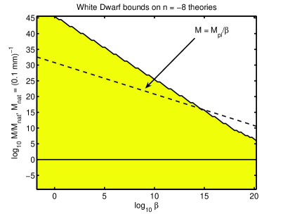
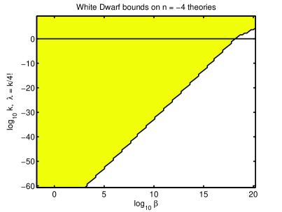
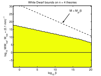
Figure 8: [Colour Online] Constraints on chameleon theories coming from white dwarfs and neutron stars. The shaded area shows the regions of parameter space that are allowed assuming that any alterations to the white-dwarf mass-radius relationship are at the $5\%$ level or smaller and that the chameleon only induces changes that are smaller than $10\%$ in the maximum white-dwarf density, $\rho_{crit}$. Neutron star bounds are not competitive with the white-dwarf constraints. The solid black lines indicate the cases where $M$ and $\lambda$ take ‘natural values’. The dotted-black line indicates when $M=M_{\phi}:=M_{pl}/\beta$ i.e. when the mass scale of the potential is the same as that of the matter coupling. Other $n<-4$ theories are similar to the $n=-8$ case, whilst the $n=4$ plot is typical of what is allowed for $n>0$ theories. The amount of allowed parameter space increases with $|n|$.

We define $B=k_{1}K$, $C=k_{2}M_{pl}^{-2}$, $D=k_{3}m_{e}^{2}/m_{u}^{2/3}$ and $F=k_{4}M_{pl}^{-4}$. We also define $H=\alpha_{\phi}/|{n}||\beta\phi(\rho_{c})M_{pl}^{-1}|\rho_{c}^{1/(n+1)}$. As defined, $H$ is actually independent of $\rho_{c}$. With these definitions, the energy is extremised when:

$$\frac{dE}{d\rho_{c}}=\tfrac{1}{3}(BM_{star}-CM_{star}^{5/3})\rho_{c}^{-2/3}-\tfrac{1}{3}DM_{star}\rho_{c}^{-4/3}-\tfrac{2}{3}FM_{star}^{7/3}\rho_{c}^{-1/3}-HM_{star}\rho_{c}^{-\frac{n+2}{n+1}}=0.$$

At leading order, we drop the terms proportional to $D$, $F$ and $H$ and recover the standard Chandrasekar limit for the mass of a white dwarf:

$$M_{star}=\left(\frac{A}{B}\right)^{3/2}=1.457\left(\frac{\mu_{e}}{2}\right)^{-2}M_{\odot},$$

where $M_{\odot}$ is the mass of the Sun. Instability begins to occur when ${\mathrm{d}}^{2}E/{\mathrm{d}}^{2}\rho_{c}=0$ which, given that ${\mathrm{d}}E/{\mathrm{d}}\rho_{c}=0$, is equivalent to:

$$\frac{2}{3}D\rho_{c}^{-4/3}-\frac{2}{3}FM^{4/3}_{star}\rho_{c}^{-1/3}+\frac{n+4}{n+1}H\rho_{c}^{-\frac{n+2}{n+1}}=0.$$ (42)

Solving this equation for $\rho_{c}$ gives a critical density, $\rho_{crit}$, at which instability occurs. We find that, for all $n\neq-4$, there will be a chameleon induced correction to $\rho_{crit}$. When $n\neq-4$, we must either have $n\leq-6$ or $n>0$ and so then $(n+2)/(n+1)>4/5>1/3$. This observation means that eq. (42) still has solutions. The effect of the chameleon is to raise the value of $\rho_{crit}$. Even in pure General Relativity it turns out that this critical density is so high that it will only be important for white dwarfs in which the core is ${}^{4}{\mathrm{He}}$, bholes . In all other cases, except for that where the core is ${}^{12}{\mathrm{C}}$, $\rho_{crit}$ is greater than the neutronisation threshold, and so such high-density white dwarfs will not occur. In the case of carbon white dwarfs, the central density is in fact limited by pyconuclear reactions, bholes . Since the addition of a chameleon field raises $\rho_{crit}$, this change can only be potentially important for Helium white dwarfs.

If the effect of the chameleon is small then, at leading order, $\rho_{crit}=CB^{2}/DA^{2}=2.65\times 10^{10}\,{\mathrm{g\,cm}}^{-3}$ for ${}^{4}{\mathrm{He}}$ stars. The leading order chameleon correction to $\rho_{crit}$ is

$$\frac{\delta\rho_{crit}}{\rho_{crit}} = \frac{3(n+4)}{2(n+1)}\left(\frac{\alpha_{\phi}(2m_{u})^{2/3}\rho_{crit}^{1/3}}{|n|m_{e}^{2}k_{3}}\right)\left|\frac{\beta\phi(\rho_{crit})}{M_{pl}}\right|$$

$$= 1.33\times 10^{-44}\frac{(n+4)}{(n+2)}\alpha_{\phi}\left(\frac{1.22\beta\times 10^{12}}{|n|}\right)^{\frac{n}{n+1}}\left(\frac{M}{1\,{\mathrm{mm}}^{-1}}\right)^{\frac{n+4}{n+1}}.$$

If we wish to require that the presence of a chameleon do little to alter the stability properties of white dwarfs in general relativity, we will need $\delta\rho_{crit}/\rho_{crit}\ll 1$. This gives us another upper bound on $\beta$. In general, however, it is not competitive with the white-dwarf mass-radius relation bound on $\beta$. The requirement $\delta\rho_{crit}/\rho_{crit}<0.1$ is included in the plots of FIG. 8.

VII.3 Discussion

It should be noted that, in this section, the bounds that have been derived on $\beta$ have been found under the assumption that the chameleon field couples to relativistic matter in the same way as it does to normal matter i.e. it just couples to the rest mass energy density of matter. As we noted in the introduction, however, it is usually the case that the chameleon in fact couples to some linear combination of the energy density and the pressure e.g. $\rho+\omega P$. In the simplest models $\omega=-3$. The total energy density, $\rho_{tot}$, of the star with equation of state $P=K\rho_{0}^{\Gamma}$ is given by:

$$\rho_{tot}=\rho_{0}+\frac{P}{\Gamma-1}=\rho_{0}+pP$$

where $\rho_{0}$ is the rest mass energy density and $\Gamma=1+1/p$. In calculations presented above, we have implicitly assumed that $\rho_{tot}+\omega P=\rho_{0}+(p+\omega)P\approx\rho_{0}$. The bounds that we have derived come from the sector where the matter in the star is relativistic i.e. $p=3$. If the chameleon couples to matter through the trace of the energy momentum tensor i.e. $\omega=-3$ then we do, in fact, have $\rho_{tot}=\rho_{0}$, just as we have assumed.

In the non-relativistic case, $P\ll\rho_{0}$, and so $\rho_{tot}+\omega P\approx\rho_{0}$ is always true. Even in the relativistic case, since $P/\rho=K\rho_{0}^{1/3}\ll 1$ for white dwarfs, and $P/\rho=K\rho_{0}^{1/3}\sim\mathcal{O}(1)$ for neutron stars, we always have $P\lesssim\mathcal{O}(\rho)$, and so different values of $\omega$ will only alter our bounds by at most an $\mathcal{O}(1)$ quantity. There is one caveat: if $\omega$ is chosen so that $\rho_{tot}+\omega P$ can become negative, then the $n>0$ chameleon field theories will cease to display chameleon behaviour. This would immediately rule them out for all $\beta\gtrsim 1$.

VIII Cosmological and Other Astrophysical Bounds

VIII.1 Nucleosynthesis and the Cosmic Microwave Background

The compact object bounds present above constrain a chameleon field behaves in very high density backgrounds whereas cosmological bounds on chameleon theories constrain how the behaviour of the chameleon field in low-density backgrounds. We have assumed that the chameleon couples to the energy density and pressure of matter in the combination:

$$\rho+\omega P.$$

In the radiation era $P\approx 3\rho$. Provided then that $\rho(1+\omega/3)>0$, i.e. $\omega>-3$, and $\beta$ is large enough, the chameleon will simply stay at the minima of its effective potential, which is itself slowly evolving over time. For this to be the case it is required that:

$$\left|\square\phi_{c}\right|\ll\left|\frac{\beta\rho(1+\omega/3)}{M_{pl}}\right|,$$

where $\phi_{c}$ is the value of $\phi$ at its effective minima:

$$\phi_{c}=M\left(\frac{M^{3}M_{pl}\lambda n}{\beta\rho(1+\omega/3)}\right)^{\frac{1}{n+1}},$$

and so:

$$\square\phi_{c} = -\ddot{\phi}_{c}-3H\dot{\phi}_{c}=-\frac{4(n+5)}{(n+1)^{2}}H^{2}\phi_{c}$$

$$= -\frac{4(n+5)}{(n+1)^{2}}\left(\frac{8\pi}{3\beta^{2}(1+\omega/3)}\right)\left(\frac{\beta\phi_{c}}{M_{pl}}\right)\left(\frac{\beta\rho(1+\omega/3)}{M_{pl}}\right),$$

where we have used $H^{2}=8\pi\rho/3M_{pl}^{2}$ and $\dot{\rho}=-4H\rho$ as appropriate for the radiation era.

We shall show below that we must require that $|\beta\phi_{c}/M_{pl}|<0.1$ since the epoch of nucleosynthesis. When $\beta\gtrsim 1$, it follows from eq. (VIII.1) that this requirement is enough to ensure that $|\square\phi_{c}|\ll\beta\rho(1+\omega/3)/M_{pl}$ provided that $\omega>-3$.

The simplest, and perhaps the most natural way, for the chameleon to interact with matter in a relativistically invariant fashion, however, is for it to couple to the trace of the energy momentum tensor i.e. $\omega=-3$. When $\omega=-3$ the above analysis does not apply. The strongest bounds on the parameters of chameleon theories arise in $\omega=-3$ case.

When $\omega=-3$ we must evaluate $\rho-3P$. Although $\rho\approx 3P$ in the radiation era, $\rho-3P$ is not identically zero. Following chameleoncosmology , we find, for each particle species $i$:

$$\rho_{i}-3P_{i}=\frac{45}{\pi^{4}}\frac{H^{2}M_{pl}^{2}}{8\pi}\frac{g_{i}}{g_{\ast}(T)}\tau(m_{i}/T),$$

where $g_{\ast}=\sum_{bosons}g_{i}^{boson}(T_{i}/T)^{4}+(7/8)\sum_{fermions}g_{i}^{fermion}(T_{i}/T)^{4}$ is the standard expression for the total number of relativistic degrees of freedom; $g_{i}$ and $T_{i}$ are respectively the degrees of freedom and temperature of the $i$th particle species. The function $\tau$ is defined by:

$$\tau(x)=x^{2}\int_{x}^{\infty}du\frac{\sqrt{u^{2}-x^{2}}}{e^{u}\pm 1}$$

with the $+$ sign for fermions and the $-$ for bosons. This function goes like $x^{2}$ when $x\ll 1$ and $e^{-x}$ when $x\gg 1$, but it is $\mathcal{O}(1)$ when $x\sim\mathcal{O}(1)$. The case $\beta\sim\mathcal{O}(1)$ and $n>0$ was analysed very thoroughly in chameleoncosmology . We will therefore restrict ourselves to looking at the $n\leq-4$ cases. We will also consider, for all $n$, what new features emerge when we take $\beta\gg 1$. In both cases we will see that theories with $n\leq-4$ and/or $\beta\gg 1$ are much less susceptible to different initial conditions than those with $n>0$ and $\beta\sim\mathcal{O}(1)$.

We consider the cases $n\leq-4$ and $n>0$ separately below. Before we do so, we note some similarities between the two cases. Whatever the sign of $n$, the effective potential will have a minima at:

$$\phi_{min}(T)=M\left(\frac{M_{pl}M^{3}n\lambda}{\beta\hat{\rho}(T)}\right)^{\frac{1}{n+1}},$$

where we define:

$$\hat{\rho}(T)=\sum_{i}\left(\rho_{i}-3P_{i}\right).$$

From the form of $\rho_{i}-3P_{i}$, it is clear that $\hat{\rho}$ will be dominated by the heaviest particle species that satisfies $m_{i}\lesssim T$. When $m_{i}\ll T$, $\tau\propto(m_{i}/T)^{2}$ and so the largest value of $m_{i}$ dominates, whereas the contribution from species with $m_{i}\gg T$ are exponentially suppressed. The function $\tau(m_{i}/T)$ is peaked near $m_{i}/T=1$.

If the chameleon is not at $\phi_{min}$, and $(\phi_{min}/\phi)^{n+1}\ll 1$, then this peak will result in the value of $\phi$ being ‘kicked’ towards $\phi_{min}(T)$. We label the distance that $\phi$ moves due to this ‘kick’ by $(\Delta\phi)_{i}$ where

$$(\Delta\phi)_{i}\approx-\frac{\beta g_{i}M_{pl}}{8\pi g_{\ast}(m_{i})}\left(\begin{array}[]{l}\tfrac{7}{8}\\ 1\end{array}\right).$$

The $7/8$ is for fermions and the $1$ for bosons. This formula is valid so long as $|\phi_{min}(T)-\phi|>|\Delta\phi_{i}|$ i.e. so long as the kick is not large enough to move $\phi$ to its minimum.

The largest jump of this sort will occur for the smallest value of $g_{i}/g_{\ast}$. It will therefore occur when electrons decouple from equilibrium at $T\approx 0.5\,{\mathrm{MeV}}$. If, however, $|\phi-\phi_{min}(T)|$ is smaller in magnitude than this above quantity, then $(\Delta\phi)_{i}=\phi_{min}-\phi$. Whether or not $\phi$ will stay at $\phi_{min}(T)$, as it evolves with time, will depend on the mass of the chameleon at $\phi_{min}(T)$. If $m_{\phi}^{2}\gg H^{2}$ then it will stay at the minimum. Otherwise it will tend to slowly evolve towards values of $\phi$ for which $(\phi_{min}/\phi)^{n+1}<1$.

If $(\phi_{min}/\phi)^{n+1}>1$ then $\phi$ will very quickly (in under one Hubble time) roll down the potential. It will either overshoot $\phi_{min}$, or if the mass of the chameleon at $\phi_{min}$ is large enough, stick at $\phi_{min}$. We can therefore assume that our initial conditions are such that, in the far past, $\phi$ is either at $\phi_{min}$ or $(\phi_{min}/\phi)^{n+1}<1$.

VIII.1.1 Case $n\leq-4$

We note that when $n\leq-4$, before any jump, we have $\phi_{min}/\phi>1$ and so $|\phi_{min}-\phi|\leq|\phi_{min}|$. It follows that:

$$\frac{\phi_{min}(T\approx m_{i})}{(\Delta\phi)_{i}}\approx\frac{45(n+1)}{\pi^{4}}\frac{H^{2}(T\approx m_{i})}{m_{\phi}^{2}(\phi_{min})}.$$

This seems to suggest that, if $(\Delta\phi)_{i}$ is large enough to move $\phi$ to $\phi_{min}(T)$, then we will necessarily have $m_{\phi}^{2}(\phi_{min})>H^{2}$, and so $\phi$ will stay at $\phi_{min}(T)$ in the subsequent evolution. However, this is not quite the case. As $T$ drops below $m_{i}$, the $i$th species decouples and its energy density decreases exponentially. This causes $\hat{\rho}$, and consequently $m_{\phi}(\phi_{min}(T))$, to decrease quickly. Roughly, $\hat{\rho}$ shortly after decoupling will be a factor of $(m_{j}/m_{i})^{2}$ smaller than it was before, where the $j$th species is the most massive species of particle obeying $m_{j}<m_{i}$.

If $\phi$ reaches $\phi_{min}(T\approx m_{i})$ with the $i$th kick, then as $T$ decreases the chameleon will roll quickly down to the potential towards $\phi_{min}(T<m_{i})$; $|\phi_{min}(T<m_{i})/\phi_{min}(T\approx m_{i})|<1$. For $\phi$ to stick at $\phi_{min}$, for $m_{j}<T<m_{i}$, and not overshoot it, we need:

$$\frac{H^{2}(T)}{m_{\phi}^{2}(\phi_{min}(T))}\approx\left(\frac{T}{m_{i}}\right)^{\frac{2n}{n+1}}\left(\frac{m_{i}}{m_{j}}\right)^{\frac{2(n+2)}{n+1}}\frac{H^{2}(m_{i})}{m_{\phi}^{2}(\phi_{min}(m_{i}))}\ll 1.$$

Since $T<m_{i}$ in this region, and $n/(n+1)>0$, it is sufficient to require:

$$\left(\frac{m_{i}}{m_{j}}\right)^{\frac{2(n+2)}{n+1}}\frac{H^{2}(m_{i})}{m_{\phi}^{2}(\phi_{min}(m_{i}))}\ll 1.$$

We know that $m_{\phi}\propto\beta^{(n+2)/(n+1)}$ and so the above condition is more likely to be satisfied for larger values of $\beta$ than for smaller ones.

We note that, even when $\phi\neq\phi_{min}$, we cannot have $\phi/\phi_{min}\gg 1$. If this were the case initially, when $\phi=\phi_{i}$ say, then the gradient in the $\phi$ potential would be very steep and in one Hubble time $\phi$ would move a distance $\Delta\phi$ where:

$$\frac{\Delta\phi}{\phi_{i}}\sim-\beta\left(\frac{m_{i}}{T}\right)^{2}\left(\frac{M_{pl}}{\phi_{min}}\right)\left(\frac{\phi_{min}}{\phi_{i}}\right)^{(n+2)}.$$

It is clear from this expression that for $\beta\gtrsim\mathcal{O}(1)$, $\phi/\phi_{min}$ will decrease very quickly and pretty soon $\phi/\phi_{min}\lesssim 1$.

When $\beta\gtrsim\mathcal{O}(1)$ it is therefore valid to assume that, for almost of all of the radiation era evolution, $\phi(T)/\phi_{min}(T)\lesssim 1$. The larger $\beta$ becomes, the greater the extent to which this assumption holds true.

The main purpose of the above discussion is to illustrate that, for theories with $n\leq-4$, the late time behaviour of $\phi$ will be virtually, independent of one’s choice of initial conditions. The same is not true, or at least not true to the same extent, of theories in which $n>0$. The corollary of this result is that $|\beta\phi/M_{pl}|$ could be very large at the beginning of the radiation epoch and still be less than 0.1 from the epoch of nucleosynthesis onwards. This would correspond to the masses of particles during the early radiation era being very different from the values they have taken since the epoch of nucleosynthesis until the present day. The larger $\beta$ is, the easier it is to support large changes in the particle masses. This is one reason why $\beta\gg 1$ is theoretically very interesting. In chameleon theories with $\beta\gg 1$, the constants of nature that describe the physics of the very early universe (i.e. pre-nucleosynthesis) could take very different values from the ones that they do today. This could have some interesting implications for baryogenesis at the electroweak scale.

The best radiation-era bounds on $\beta,M$ and $\lambda$ come from big-bang nucleosynthesis (BBN) and the isotropy of the cosmic microwave background (CMB). As noted in chameleoncosmology , a variation in the value of $\phi$ between now and the epochs of BBN and recombination would result in a variation of the particle masses (relative to the Planck mass) of about:

$$\left|\frac{\Delta m}{m}\right|\sim\frac{\beta|\Delta\phi|}{M_{pl}}.$$

BBN constrains the particle masses at nucleosynthesis to be within about 10% of their current values, chameleoncosmology . This requires:

$$|\phi_{BBN}|\lesssim 0.1\beta^{-1}M_{pl}.$$

We have argued above that $\phi_{BBN}/\phi_{min}(T_{BBN})\lesssim 1$ and so the above condition will be satisfied whenever:

$$|\phi_{min}(T_{BBN})|\lesssim 0.1\beta^{-1}M_{pl}.$$

Nucleosynthesis occurs at temperatures between $0.1\,{\mathrm{MeV}}$ and $1.3\,{\mathrm{MeV}}$. Since $\phi_{min}(T)$ decreases with temperature, we conservatively evaluate the above condition with $T_{BBN}=2\,{\mathrm{MeV}}$. At such temperatures the largest contribution to $\hat{\rho}$ will come from the electrons (with $m_{e}(today)=0.511\,{\mathrm{MeV}}$) and:

$$\hat{\rho}\approx\frac{g_{e}T^{2}m_{e}^{2}}{24}\approx\frac{g_{e}({\mathrm{MeV}})^{4}}{24},$$

where $g_{e}=4$ ($2$ from the electrons and $2$ from the positrons). The BBN constraint on $\beta$, $\lambda$ and $M$ for $n\leq-4$ is therefore:

$$\lambda|n|\left(\frac{1.8\beta\times 10^{6}}{\lambda|n|}\right)^{\frac{n}{n+1}}\left(\frac{M}{1\,{\mathrm{mm}}^{-1}}\right)^{\frac{n+4}{n+2}}\lesssim 1.1\times 10^{37}.$$

This is, however, a weaker bound on $\{\beta,M,\lambda\}$ than the white dwarf mass-radius relation constraint discussed in section VII above.

Another important restriction on these chameleon theories comes out of considering the isotropy of the CMB wmap . As is mentioned in chameleoncosmology a difference between the value of $\phi$ today and the value it had during the epoch of recombination would mean that the electron mass at that epoch differed from its present value $\Delta m_{e}/m_{e}\approx\beta\Delta\phi/M_{pl}$. Such a change in $m_{e}$ would, in turn, alter the redshift at which recombination occurred, $z_{rec}$:

$$\left|\frac{\Delta z_{rec}}{z_{rec}}\right|\approx\left|\frac{\beta\Delta\phi}{M_{pl}}\right|.$$

WMAP bounds $z_{rec}$ to be within 10% of the value that has been calculated using the present day value of $m_{e}$, chameleoncosmology . We define $\hat{\rho}_{rec}$ and $\hat{\rho}_{BBN}$ to be, respectively, the value that $\hat{\rho}$ takes at the recombination and BBN epochs. Now $\hat{\rho}_{rec}\gg\rho_{today}$, where $\rho_{today}$ is the cosmological energy density, and $\phi\propto\rho^{-1/(n+1)}$, it follows that $|\Delta\phi|\approx|\phi_{rec}|$ for $n\leq-4$. $\phi_{rec}$ is the value of $\phi$ had during the epoch of recombination. However, since $\hat{\rho}_{rec}<\hat{\rho}_{BBN}$, we also have $\phi_{rec}/\phi_{BBN}<1$, and so this CMB bound is always weaker than the one coming from BBN. For this reason we do not evaluate the CMB constraint here.

VIII.1.2 Case $n>0$

When we considered theories with $n\leq-4$, the analysis was made easier by the fact that $V(\phi)$ had a minimum. This allowed us to bound the magnitude of $\phi$ to be approximately less than that of $\phi_{min}(T)$. However, when $n>0$, the potential is of runaway form and we cannot bound the magnitude of $\phi$ in such a way. Many of the issues involved with $n>0$ potentials were discussed very thoroughly in ref. chameleoncosmology . In that work it was assumed that $\beta\sim 1$ and so, generically $m_{\phi}(\phi_{min})\ll H$ in the radiation era, due the fact that $\hat{\rho}\ll\rho$. However, if $\beta\ll 1$, it is possible for $m_{\phi}$ to be large compared to $H$.

As with the $n\leq-4$ case, it is not necessary to require that $\phi$ is at its effective minima during the whole of the radiation era. All that is really needed is for $\phi$ be sufficiently close to the minima at the epochs of BBN and recombination that we are able to satisfy their constraints. It was shown in chameleoncosmology that the total sum of all of the kicks that occur before BBN will move the chameleon a distance of approximately: $\beta M_{pl}$. BBN requires that:

$$|\Delta\phi_{BBN}|=\phi_{today}-\phi_{BBN}\lesssim 0.1\beta^{-1}M_{pl}.$$

Provided that, at the beginning of the radiation era, $\phi\ll\beta M_{pl}/8\pi$, then $\phi$ at BBN will easily satisfy the above bound provided that $\beta\phi_{today}/M_{pl}<0.1$.

The first of these requirements is a statement about initial conditions. It is clear that the larger $\beta$ becomes, the less restrictive this condition is. Indeed for $\beta\gg 1$, it is quite possible to have had $\beta\phi/M_{pl}\sim 0.1\mathcal{O}(\beta^{2})\gg 1$ at the beginning of the radiation era and still satisfy this bound. The larger the matter coupling is, the less important the initial conditions become, and the greater the scope for large changes in the values of the particle masses and other constants to have occurred between the pre-BBN universe and today.

Recombination enforces a similar bound to BBN:

$$\frac{\Delta z_{rec}}{z_{rec}}\approx\frac{\beta(\phi_{today}-\phi_{rec})}{M_{pl}}\lesssim 0.1.$$

If the requirements on the initial conditions are satisfied, we will have $\phi_{today}\gg\phi_{rec},\,\phi_{BBN}$ and so, in both cases, $\Delta\phi\approx\phi_{today}$. We must therefore require that

$$\beta\phi_{today}/M_{pl}\lesssim 0.1.$$

$\phi_{today}\propto\rho_{c}^{-1/(n+1)}$ where $\rho_{c}$ is that part of the cosmological energy density of matter that the chameleon couples to. For the most part, we have, in this paper, assumed that the chameleon couples to all forms of matter with the same strength. However, up to now, we have only been concerned with baryonic matter. Even if the chameleon to baryon coupling is virtually universal, there is not necessarily any reason to expect the chameleon to couple to dark matter with the same strength. It is possible that the chameleon does not interact with dark matter at all. Since it clear that $\phi_{today}$ is a very important quantity when it comes to bounding $n>0$ chameleon theories, it is crucial to know what fraction of the cosmological energy density the chameleon actually couples to. The smaller $\rho_{c}$ is, the larger $\phi_{today}$ will be. The larger the value of $\phi_{today}$, the more restrictive the resultant bound on $\{\beta,M,\lambda\}$. This implies that cosmological bounds on a chameleon theory that couples only to baryonic matter will be stronger than those on a chameleon that also couples to dark matter. Not knowing how the chameleon couples to dark matter, we chose to be cautious, and err on the side of specifying a bound that is perhaps slightly too tight, rather than too loose. We therefore work on the assumption that the chameleon only couples to baryonic matter, and so $\rho_{c}\approx 0.42\times 10^{-30}\,{\mathrm{g\,cm}}^{-3}$, wmap . Under this assumption, we find:

$$8.34\times 10^{-3}|n|\left(\frac{1.93\times 10^{-29}\beta}{n}\right)^{\frac{n}{n+1}}\left(\frac{M}{1\,\mathrm{mm}^{-1}}\right)^{\frac{n+4}{n+1}}<1.$$

If the chameleon to dark matter coupling is similar in magnitude to the baryon coupling then $\rho_{c}\approx 2.54\times 10^{-30}\,{\mathrm{g\,cm}}^{-3}$ and we have the less restrictive bound:

$$1.39\times 10^{-3}|n|\left(\frac{1.17\times 10^{-28}\beta}{n}\right)^{\frac{n}{n+1}}\left(\frac{M}{1\,\mathrm{mm}^{-1}}\right)^{\frac{n+4}{n+1}}<1.$$

The bound that we have just found has come about from the requirement that the particle masses at BBN and recombination are within 10% of the values they take in regions of cosmological density i.e. $\rho_{today}\sim 10^{-30}\,{\mathrm{g\,cm}}^{-3}$. However, all cosmological determinations of the particle masses, and indeed of the other constants of nature, have come from analysing measurements made in regions with densities much greater than the cosmological one. For instance, recent cosmological determinations of $m_{p}/m_{e}$ have employed the absorption and emission spectra of dust clouds around QSOs reinhold ; webbmore . These dust clouds have typical densities of the order of $\rho\sim 10^{-25}-10^{-24}\,{\mathrm{g\,cm}}^{-3}$. If we take $\rho_{c}$ to be $10^{-25}\,{\mathrm{g\,cm}}^{-3}$, then the BBN and CMB bounds would only require:

$$3.52\times 10^{-8}|n|\left(\frac{4.59\times 10^{-24}\beta}{n}\right)^{\frac{n}{n+1}}\left(\frac{M}{1\,\mathrm{mm}^{-1}}\right)^{\frac{n+4}{n+1}}<1.$$

VIII.1.3 Summary

We have plotted the BBN and CMB constraints on $\{\beta,M\lambda\}$ in FIG. 9. We have plotted what occurs in the most restrictive case i.e. when the chameleon couples only to baryons. The whole of the shaded region is currently allowed.

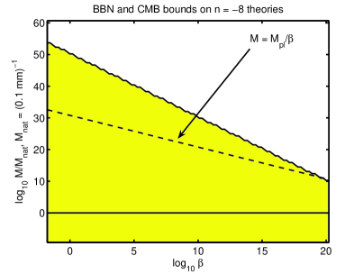
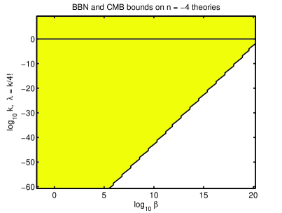
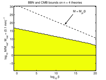
Figure 9: [Colour Online] Constraints on chameleon theories coming from the particle masses at big-bang nucleosynthesis and the constraints the redshift of recombination. The shaded area shows the regions of parameter space that are allowed by the current data. The solid black lines indicate the cases where $M$ and $\lambda$ take ‘natural values’. The dotted-black line indicates when $M=M_{\phi}:=M_{pl}/\beta$ i.e. when the mass scale of the potential is the same as that of the matter coupling. Other $n<-4$ theories are similar to the $n=-8$ case, whilst the $n=4$ plot is typical of what is allowed for $n>0$ theories. The amount of allowed parameter space increases with $|n|$. In these plots we have assumed that the chameleon couples only to baryons. Slightly weaker constraints result if the chameleon additionally couples to dark matter.

Another class of potentially important cosmological bounds can be derived by employing astronomical bounds on the allowed variation of the fundamental constants of nature during the matter era. We discuss this further below.

VIII.2 Variation of fundamental constants

Any variation in a chameleon field will lead to a variation in the masses of the particle species to which the chameleon couples. This variation is relative to the fixed Planck mass, $M_{pl}=G^{-1/2}$. If the chameleon couples to all matter particles in the same way, then all the fundamental particle masses will vary in the same fashion and so their ratios will remain constant. It is also feasible to construct theories where a variation in the chameleon leads to a variation in some other fundamental ‘constants’ of nature. For instance one might propose a theory where the fine-structure constant, $\alpha_{em}$, is given by $\alpha_{em}=f(\beta\phi/M_{pl})$ for some function $f$. If this is the case then, in addition to bounds on any allowed variation in the particle masses, we would also have to apply the whole range of very stringent bounds on the possible variation of $\alpha_{em}$ mentioned above.

For the purposes of this section, however, we assume that $\alpha_{em}$ is a true constant. It should be noted that even if $\alpha_{em}$ does vary with $\phi$ at the same level as the particle masses do, the resulting bounds on the parameters of the theory are only slightly more stringent than those already found.

The best matter era bounds on the variation of the particle masses come from measurements of the ratio $\mu=m_{p}/m_{e}$, reinhold ; webbmore ; uzan . We shall assume that the chameleon couples to protons with strength $\beta_{p}$ and to electrons with strength $\beta_{e}$. The relative change in the proton and electron masses is then given by:

$$\frac{\Delta m_{p}}{m_{p}} \approx \frac{\beta_{p}\Delta\phi}{M_{pl}},$$

$$\frac{\Delta m_{e}}{m_{e}} \approx \frac{\beta_{e}\Delta\phi}{M_{pl}}.$$

Without any a priori knowledge about the magnitude, or sign, of $\beta_{e}-\beta_{p}$ it is difficult to derive any bounds on chameleon theories simply by considering $\Delta\mu/\mu$, where $\mu=m_{p}/m_{e}$. The simplest assumption one could make about the matter coupling, $\beta$, is that it is universal i.e. $\beta_{p}=\beta_{e}=\beta$. If this is the case then $\Delta\mu=0$ identically. An alternative, but still very reasonable, assumption about the chameleon coupling, which would produce $\Delta\mu\neq 0$, is that the chameleon couples to all fundamental particles with the same universal coupling, $\beta_{U}$, but that the QCD scale, $\Lambda_{QCD}$, is independent of $\phi$. When the quark masses vanish the proton mass is proportional to $\Lambda_{QCD}$. The masses of the three lightest quarks, $m_{u}$, $m_{d}$ and $m_{s}$, are considerably smaller than $\Lambda_{QCD}$ and as a result contribute only a small correction to the proton mass (at approximately the 10% level). If $\Lambda_{QCD}$ is $\phi$-independent, we expect the proton mass to depend only weakly on $\phi$, through the quark masses, and so $\beta_{p}\sim\mathcal{O}(\beta_{U}/10)$ whereas $\beta_{e}=\beta_{U}$. Since the mass of the electron is so much smaller than the proton mass, the coupling of the chameleon to baryons is approximately given by $\beta_{p}$, and so it is $\beta_{p}$ that is constrained by the experiments mentioned in sections VI and VII. However, the BBN and CMB requirements constrain $\beta_{e}=\beta_{U}$. A change in $\phi$ of $\Delta\phi$ would therefore induce a change in $\mu$ of:

$$\frac{\Delta\mu}{\mu}\approx-9\frac{\beta\Delta\phi}{M_{pl}}.$$ (45)

As we reported above, the Reinhold et al., reinhold , result is consistent with a difference between the laboratory value of $\mu$ and the one measured in such a dust cloud at the $3.5\sigma$ level: $\Delta\mu/\mu=2.0\pm 0.6\times 10^{-5}$ where $\Delta\mu=\mu_{dust}-\mu_{lab}$. It should be noted that in the context of the chameleon theories considered here $\Delta\phi=\phi_{dust}-\phi_{lab}$ is always positive and so $\Delta\mu/\mu<0$ if $\beta_{p}=\beta_{e}/10$ as we have assumed. Under this assumption, it is not possible to reproduce the result of Reinhold et al.. If we had alternatively assumed that the fundamental particle masses are true constants but that $\Lambda_{QCD}$ is $\phi$-dependent, then we would be able to have $\Delta\mu/\mu>0$.

We interpret the Reinhold result conservatively i.e. as limiting any variation in $\mu$ to be at or below the $2\times 10^{-5}$ level. We shall also assume that the laboratory experiments that measure $\mu$ are performed close enough to the Earth’s surface that the background value of $\phi$ for these experiments is approximately the value the chameleon takes inside the Earth. This is last assumption is also a conservative one i.e. it will result in a tighter bound on the chameleon theory parameters. Taking the density of Earth to be $\rho_{Earth}\approx 5.5\,{\mathrm{g\,cm}}^{-3}$ and the density of the dust clouds from which the absorption spectra come to be $\rho_{dust}\sim 10^{-25}\,{\mathrm{g\,cm}}^{-3}$ we find that we must require:

$$2.88 \times 10^{-29}|n|\left(\frac{253\beta}{|n|}\right)^{\frac{n}{n+1}}\left(\frac{M}{1\,\mathrm{mm}^{-1}}\right)^{\frac{n+4}{n+1}}\lambda^{\frac{1}{n+1}}<1,\qquad n\leq-4$$

$$\beta < 1.42\lambda^{-1/4}\times 10^{19},\qquad n=-4,$$

$$1.58 \times 10^{-3}|n|\left(\frac{4.59\times 10^{-24}\beta}{n}\right)^{\frac{n}{n+1}}\left(\frac{M}{1\,\mathrm{mm}^{-1}}\right)^{\frac{n+4}{n+1}}<1,\qquad n>0.$$

For fixed $M$ and $\lambda$ this places an upper-bound on $\beta$. When $n>0$, the bounds coming from varying-$\mu$ are competitive with the other cosmological constraints and they provide a weak upper bound on $\beta$. When $n\leq-4$, however, the white dwarf bounds of section VII still provide the best upper bound on $\beta$. It should be noted that the bounds on $\{\beta,M,\lambda\}$ deduced from measurements of $\Delta\mu/\mu$ are highly model-dependent. For this reason we do not plot them here.

IX Combined bounds on chameleon theories

All of the chameleon theories considered in this work have a two-dimensional parameter space, spanned either by $M$ and $\beta$ ($n\neq-4$), or by $\lambda$ and $\beta$ ($n=-4$). We combine the constraints found in sections VI-VIII to bound the values of $\beta$ and $M$ (or $\lambda$) for different $n$. We plotted the constraints for $n=-8,\,-6,\,-4,\,1\,4$ and $n=6$ in FIG. 10. In these figures we have included all the bounds coming from the Eöt-Wash experiment, EotWash ; Eotnew , as well as those coming from Casimir force searches, Lamcas ; Decca . We also include the bounds (labeled Irvine) coming from another search for Yukawa forces, Irvine . We also show how current WEP violation experiments constrain these theories - i.e. experiments that have actually been done as opposed to the putative WEP violation experiment described in section VI.3. The white-dwarf and BBN constraints are also included in the plots, however, for these theories, they are always weaker than those laboratory tests (when $\beta\lesssim 10^{20}$). The plots for other $n<-4$ theories are very similar to the $n=-8$ and $n=-6$ plots, whilst the $n=4$ and $n=6$ cases are representative of $n>0$ theories. In general, the larger $|n|$ is, the larger the region of allowed parameter space. This is because, in a fixed density background, the chameleon mass, $m_{c}$, scales as $|n+1|^{1/2}/|n|^{1/2(n+1)}$, and so $m_{c}$ increases with $|n|$. The larger $m_{c}$ is, in a given background, the stronger the chameleon mechanism, and a stronger chameleon mechanism tends to lead to looser constraints.

We have indicated on each plot how the variety of different bounds, considered above, combine to constrain the theory. In each plot, the whole of the shaded area indicates the allowed values of $M$ and $\beta$ (or $\lambda$ and $\beta$). Three satellite experiments (SEE SEE , STEP STEP and GG GG ) are currently in the proposal stage, whilst a fourth one (MICROSCOPE MICRO ) will be launched in 2007. These experiments will be able to detect WEP violations down to $\eta=10^{-18}$. The more lightly shaded region on the plots indicates those regions of parameter space that could be detected by these experiments - we have assumed that their WEP violation experiments to be along the lines of the putative experiment described in section VI.3.

In $n>0$ theories, the increased precision, promised by these satellite tests, is not the only advantage that they offer over their lab-based counterparts. In space, the background density is much lower than in the laboratory. As a result, the thin-shell condition, eq,. (19b), is generally more restrictive for bodies in the vacuum of space than it is for the same bodies here on Earth. It is therefore possible for test-bodies, that had thin-shells in the laboratory, to lose them when they are taken into space chama ; cham1 ; chameleoncosmology . If such a thing occurs for the test-masses used in the aforementioned satellite experiments, then it is possible that they might see WEP violations in space at a level that had previously been thought ruled out by Earth-based tests i.e. $\eta>10^{-13}$. This interesting feature of $n>0$ chameleon theories was first noted in chama . It is important to stress that this effect will not occur if $\beta$ is so large that the satellites themselves develop thin-shells chama ; cham1 .

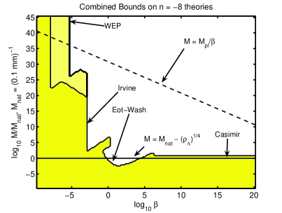
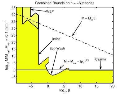
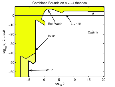
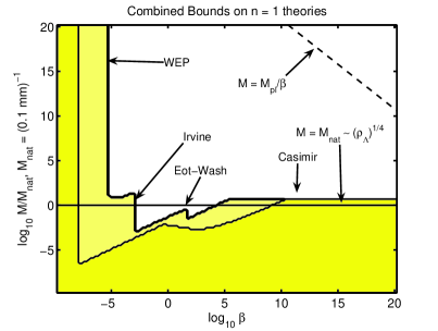
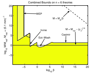
Figure 10: [Colour Online] Combined constraints on chameleon theories. The whole of shaded area shows the regions of parameter space that are allowed by the current data. Future space-based tests could detect the more lightly shaded region. The solid black lines indicate the cases where $M$ and $\lambda$ take ‘natural values’. For $n\neq-4$, a natural value for $M$ is required if the chameleon is to be dark energy. The dotted-black line indicates when $M=M_{\phi}:=M_{pl}/\beta$ i.e. when the mass scale of the potential is the same as that of the matter coupling. Other $n<-4$ theories are similar to the $n=-6$ and $n=-8$ cases, whilst the $n=4$ and $n=6$ plots are typical of what is allowed for $n>0$ theories. The amount of allowed parameter space increases with $|n|$.

In chameleon theories where the potential has a minimum, i.e. $n\leq-4$, the thin-shell condition, eqs. (19a & c), is only weakly dependent on the background density of matter. As a result, $n\leq-4$ theories will generally be oblivious to the background in which the experimental tests of it are conducted. It is for this reason that future space-based tests will be better able to constrain $n>0$ theories than they will $n\leq-4$ ones.

In all of the plots, we show $\beta$ running from $10^{-10}$ to $10^{20}$. $\beta<10^{-10}$ will remain invisible to even the best of the currently proposed space-based tests, and $\beta>10^{20}$ corresponds to $M_{pl}/\beta<500\,{\mathrm{MeV}}$. The region in which $M_{pl}/\beta\lesssim 200\,{\mathrm{GeV}}$ is, in fact, probably already ruled out. If $\beta$ were so large that $M_{pl}/\beta<200\,{\mathrm{GeV}}$, then we would probably have already seen some trace of the chameleon in particle colliders. This said, without a quantum theory for the chameleon it is hard to say how chameleon theories behave at high energies. A result a detailed calculation of the chameleon’s effect on scattering amplitudes is not possible at this stage. A full quantum mechanical treatment of the chameleon is very much beyond the scope of this work, but remains one possible area of future study.

The chameleon mass ($m_{c}$), in a background of fixed density, scales as $\lambda^{\frac{n}{n+1}}M^{-\frac{n+4}{2(n+1)}}$. As we mentioned above, the larger $m_{c}$, is the easier it is to satisfy the thin-shell conditions, eqs. (19a-c), and the stronger the chameleon mechanism becomes. Since $(n+4)/(2(n+1))\geq 0$ and $n/(n+1)>0$, for all theories considered here, the chameleon mechanism becomes stronger as $M\rightarrow 0$, or $\lambda\rightarrow\infty$, and all of the constraints are more easily satisfied in these limits. It is for this reason that we truncate our plots for some small $M$ and, when $n=-4$, for a large value of $\lambda$. Values of $M$ that are smaller than those shown, or values of $\lambda$ that are larger, are still allowed.

The upper limit on $M$ (and lower limit on $\lambda$) has been chosen so as to show as much of the allowed parameter space as possible. When $\beta$ is very small, the chameleon mechanism is so weak that, in all cases, $\phi$ behaves like a standard (non-chameleon) scalar field. When this happens, the values of $M$ and $\lambda$ become unimportant, and the bounds one finds are on $\beta$ alone. This transition to non-chameleon behaviour can be seen to occur towards the far left of each of the plots.

It is clear from FIG. 10 that $\beta\gg 1$ is, rather unexpectedly, very much allowed for a large class of chameleon theories. We can also see that, rather disappointingly, future space-based searches for WEP violation, or corrections to $1/r^{2}$ behaviour of Newton’s law, will only have a small effect in limiting the magnitude of $\beta$. If $M_{pl}/\beta\sim 1\,{\mathrm{TeV}}$ is feasible, pending a detailed calculation of chameleon scattering amplitudes, that chameleon particles might be produced at the LHC.

The solid black line on each of the plots indicates the ‘natural’ values of $M$ and $\lambda$ i.e. $M\sim(0.1\,{\mathrm{mm}})^{-1}$ and $\lambda=1/4!$. The Eöt-Wash experiment and measurements of the Casimir force rule out $\lambda=1/4!$ in $\phi^{4}$, however (expect when $n=-6$) $M\sim(0.1mm)^{-1}$ is allowed for all $10^{4}\lesssim\beta\lesssim 10^{18}$. In particular, $M_{pl}/\beta\sim 10^{15}\,{\mathrm{GeV}}\approx M_{GUT}$, i.e. the GUT scale, and $M_{pl}/\beta\sim 1\,{\mathrm{TeV}}$ are allowed.

The dotted black line indicates the cases where $M=M_{pl}/\beta$ i.e. when there is only one mass scale associated with the chameleon theory. It is clear, however, that no such theories are allowed if $\beta\lesssim 10^{20}$. In all cases we must require $M\ll M_{pl}/\beta$. As noted in chama ; cham1 , this requirement introduces a hierarchy problem in the chameleon theory itself. This problem is not, however, present in $\phi^{4}$ ($n=-4$) theory.

The larger $\beta$ is the stronger the chameleon mechanism becomes. A strong chameleon mechanism results in larger chameleon masses, and larger chameleon masses in turn result in weaker chameleon-mediated forces. A stronger chameleon mechanism also increases the likelihood of the test masses, used in the experiments consider in section VI, having thin-shells. Large values of $\beta$ cannot, therefore be detected, at present by the Eöt-Wash and WEP tests, if $\lambda$ and $M$ take natural values. It is for this reason that, as can be seen in FIG. 10, the Eöt-Wash experiment and the WEP violation searches place the greatest constraints on the parameter space in a region about $\beta\sim{\mathcal{O}}(1)$. Casimir force tests are much better able to detect large $\beta$, but they can ultimately only place an upper-bound on $M$ or $1/\lambda$.

For large $\beta$, Casimir force test succeed where the Eöt-Wash experiment fails because in the former does not use a thin metal sheet to cancel electrostatic effects. If it were not for the presence of the BeCu sheet, the Eöt-Wash test would be able to detect, or rule out, almost all $\beta\gg 1$ theories with $M\sim(\rho_{\Lambda})^{1/4}$.

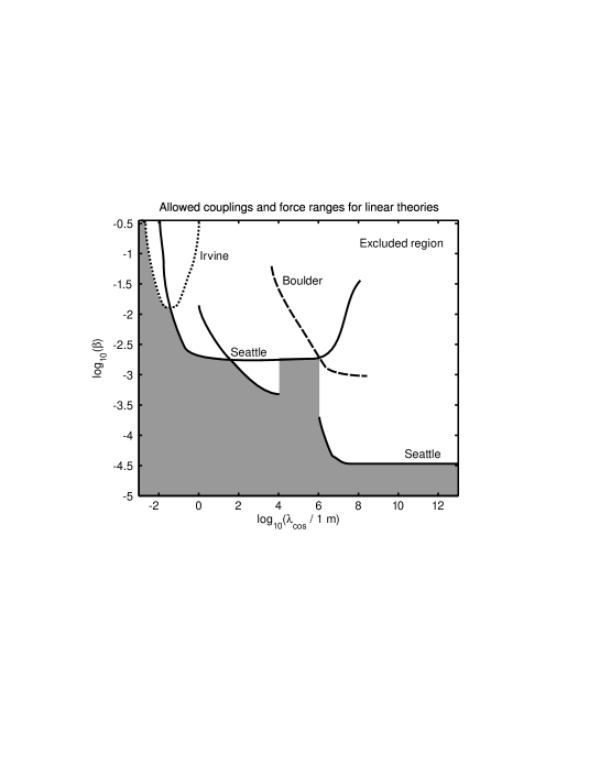
Figure 11: Allowed couplings and force ranges for scalar fields which couple to baryon number and have approximately linear field equations. The shaded area shows the parameter space that is allowed by the current bounds on scalar field theories with linear field equations. $\lambda=1/m$ is the range of the force, and $m$ is the mass of the scalar field. $\beta$ is the matter coupling of the scalar. $\beta>1$ is ruled out for all but the smallest ranges (currently $\lambda<10^{-4}{\mathrm{m}}$). We refer the reader to EotWash for a plot of the allowed parameter space for $\lambda<10^{-3}{\mathrm{m}}$. Irvine, Seattle and Boulder refers to Irvine , WEP ; WEP1 ; WEP2 and Boulder respectively.

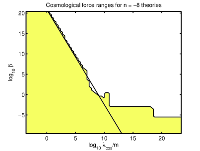
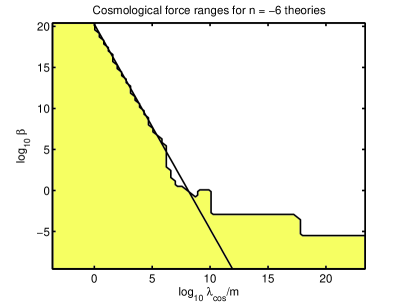
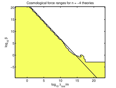
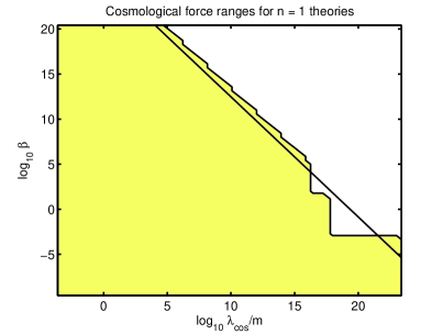
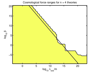
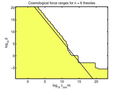
Figure 12: [Colour Online] Allowed couplings and cosmological force ranges for chameleon theories. The shaded area shows the allowed parameter space with all current bounds. $\lambda_{cos}$ is the range of the chameleon force in the cosmological background with density $\rho\sim 10^{-29}\,{\mathrm{g\,cm}}^{-3}$. It is related to the cosmological mass of the chameleon, $m_{c}^{cos}$, by $\lambda_{cos}=1/m_{c}^{cos}$. The solid black lines indicate the cases where $M$ and $\lambda$ take ‘natural’ values. Plots for theories with $n<-4$ or $n>0$ are similar to the cases $n=-8,\,-6$ and $n=4,\,6$ respectively.

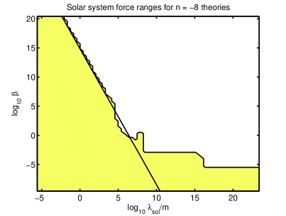
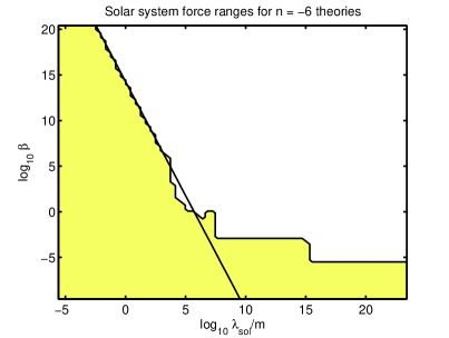
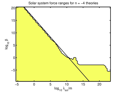
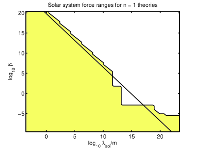
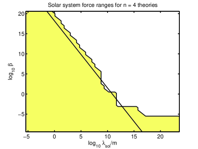
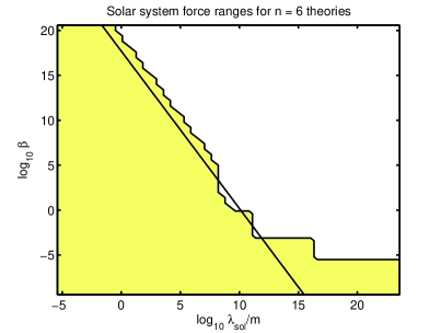
Figure 13: [Colour Online] Allowed couplings and cosmological force ranges for chameleon theories. The shaded area shows the allowed parameter space with all current bounds. $\lambda_{sol}$ is the range of the chameleon force in the solar system, where the average density of matter is $\rho\sim 10^{-24}\,{\mathrm{g\,cm}}^{-3}$. It is related to the cosmological mass of the chameleon, $m_{c}^{sol}$, by $\lambda_{sol}=1/m_{c}^{sol}$. The solid black lines indicate the cases where $M$ and $\lambda$ take ‘natural’ values. Plots for theories with $n<-4$ or $n>0$ are similar to the cases $n=-8,\,-6$ and $n=4,\,6$ respectively.

The fact that we can have $\beta\gg 1$, in scalar theories with a chameleon mechanism, is entirely due to the non-linear nature of these theories. Almost all the quoted bounds on the coupling to matter are for scalar field theories with linear field equations. In such theories $\phi$ evolves according to:

$$-\square\phi=m_{c}^{2}\phi+\frac{\beta\rho}{M_{pl}},$$

where the field’s mass, $m$, is constant (i.e. not density dependent). The $\phi$-force between two bodies with masses ${\mathcal{M}}_{1}$ and ${\mathcal{M}}_{2}$, which are separated by a distance $d$, takes the Yukawa form

$$F_{12}=\frac{\beta^{2}(1+d/\lambda)e^{-d/\lambda}{\mathcal{M}}_{1}{\mathcal{M}}_{2}}{M_{pl}^{2}d^{2}}.$$

where $\lambda=1/m_{c}$ is the range of the force. The best limits of $\lambda$ and $\beta$ come from WEP violation searches, WEP ; WEP1 ; WEP2 ; LLR ; LLR1 , and searches for corrections to the $1/r^{2}$ behaviour of gravity, EotWash . The 95% confidence limits on $m$ and $\beta$ for such a linear theory, where the field couples to baryon number, are plotted in FIG. 11 with the allowed regions shaded and the excluded regions left white. It is clear that $\beta>1$ is ruled out for all but the smallest ranges (currently $\lambda\lesssim 10^{-4}\,{\mathrm{m}}=0.1\,{\mathrm{mm}}$).

To make the comparison with the linear case more straightforward, we have replotted the allowed parameter space for chameleon theories with $n=-8,\,-6,\,-4,\,4$ and $n=6$ in terms of its coupling to matter, $\beta$, and the range of the chameleon force cosmologically, $\lambda_{cos}$, and in the solar system, $\lambda_{sol}$, in FIGS. 12 and 13. FIG. 12 shows the cosmological range, whilst $\lambda_{sol}$ is shown in FIG. 13. The solid black line, in each of these plots, indicates the case where $M$ and $\lambda$ take their ‘natural’ values. We can clearly see that, in stark contrast to the linear case, chameleon theories are easily able to accommodate both $\beta\gg 1$ and $\lambda\gg 1\,{\mathrm{m}}$. This underlines the extent to which non-linear scalar field theories are different from linear ones, and the important rôle that is played by the chameleon mechanism.

X Conclusions and Discussion

In this article we have investigated scalar field theories in which the field is strongly coupled to matter. In particular, we have studied the so called chameleon scalar fields. A scenario presented by Khoury and Weltman cham1 that employed self-interactions of the scalar-field to avoid the most restrictive of the current bounds on such fields and its coupling. In the models that they proposed, these fields would couple to matter with gravitational strength, in harmony with general expectations from string theory, whilst, at the same time, remaining very light on cosmological scales. In this work we went much further and show, contrary to most expectations, that the scenario presented in cham1 allows scalar fields, which are very light on cosmological scales, to couple to matter much more strongly than gravity does, and yet still satisfy all of the current experimental and observational constraints.

Previous investigations on such scenarios, chama ; chameleoncosmology ; nelson ; phi4 , noted that an important feature of chameleon field theories is that they make unambiguous and testable predictions for near-future tests of gravity in space. This is timely as there are currently four satellite experiments either in the proposal stage or due to be launched shortly (SEE SEE , STEP STEP , GG GG and MICROSCOPE MICRO ). A reasonably sized region of the parameter space of the chameleon theories considered here will be visible to these missions. Theories with very large couplings $\beta\gg 1$ will, however, remain undetectable. The ability of these planned missions to detect large $\beta$ theories could, however, be exponentially increased if the experiments they carry were to be redesigned slightly in the light of our findings.

Previous studies claimed that typical test masses in the above satellite experiments do not have a thin shell. Therefore, the extra force is comparable to their gravitational interaction. The chameleon model hence predicts that MICROSCOPE, STEP and GG could measure violations of the weak equivalence principle that are stronger than currently allowed by laboratory experiments. Furthermore, the SEE project could measure an effective Newton’s constant different, by order of unity, from that measured on Earth. We have seen, in this paper, that both of these features are very much properties of chameleon theories with runaway ($n>0$) potentials. They will not, in general, occur if the chameleon potential has a minimum (e.g. $n<-4$ theories). These features are also very much associated with a gravitational strength chameleon coupling i.e. $\beta\sim{\mathcal{O}}(1)$, and will not occur if $\beta\gg 1$, or $\beta\ll 1$.

The major result, presented in this work, is that current experiments do not limit the coupling of the chameleon to matter, $\beta$, to be order ${\mathcal{O}}(1)$ or smaller. Indeed, if we wish to have a ‘natural’ value of $M$ in a $V\propto\phi^{-1}$ theory then we must require $\beta\gtrsim 10^{4}$ (or $\beta\lesssim 10^{-3}$. If $\beta\gg 1$, the test-masses in the planned satellite experiments will still have thin-shells. As such SEE, STEP, GG and MICROSCOPE, as they are currently proposed, will be unable to detect the chameleon and place an upper-bound on $\beta$.

We have shown that upper-bounds on the matter coupling, $\beta$, can be derived from astrophysical and cosmological considerations. Also, if $\beta$ is very large, of the order of $10^{17}$ or greater, then it might even be possible to detect the effect on the chameleon on scattering amplitudes in particle colliders. This possibility is one avenue that requires further in depth study.

We noted in the introduction that $\beta\gg 1$ could be seen as being pleasant in light of the hierarchy problem HP ; HP1 ; HP2 . If a chameleon with a large $\beta$ where detected, it would imply that new physics emerges at a sub-Planckian energy-scale: $M_{\phi}=M_{pl}/\beta$.

A large value of the matter coupling is also preferable to an order unity value in that it leads to the late time behaviour of the chameleon being much more weakly dependent on the initial conditions, than it would be if $\beta\lesssim{\mathcal{O}}(1)$.

The magnitude of $\beta(\Delta\phi=\phi_{1}-\phi_{2})/M_{pl}$ quantifies the relative amount by the particle masses differ between a region where $\phi=\phi_{1}$ and one where $\phi=\phi_{2}$. The larger the coupling is then, the easier it is for there to have been a very large difference between the current values of particle masses, and the values that they had in the very early universe (i.e. pre-BBN). If the particle masses were very different from their present values at, say, the epoch of the electroweak phase transition, then the predictions of electroweak baryogenesis could be significantly altered.

In this paper have taken the chameleon potential to have a power-law form i.e $V\propto\phi^{-n}$. This is certainly not the only class of chameleon potentials that it is possible to have. In general, any potential that satisfies $\beta V_{,\phi}<0$, $V_{,\phi\phi}>0$ and $V_{,\phi\phi\phi}/V_{,\phi}>0$ in a region near some $\phi=\phi_{0}$ will produce a chameleon theory. In fact, a generic potential might contain many different regions in which chameleon behaviour is displayed. In some of these regions, the potential may appear to have a runaway form, and so behave qualitatively as an $n>0$ theory. In other regions, the potential might have a local minimum, leading to $n\leq-4$ type behaviour. The existence of the matter coupling provides one with a mechanism, along the lines of that considered by Damour and Polyakov pol , by which the scalar field $\phi$ can, during the radiation era, be moved into a region where it behaves like a chameleon field. The larger $\beta$ is, the more effective this mechanism becomes. Given this mechanism, one important avenue for further study is to see precisely how general late-time chameleon behaviour is of a generic scalar field theory with a strong coupling to matter.

In this paper we have avoided the temptation to linearise the chameleon field equation, eq. (9), when it is not valid to do so. We have, instead, combined matched asymptotic expansions with approximate analytical, and exact numerical, solution of the full non-linear equations to study the behaviour of chameleon field theories in more detail.

The main results of this analysis were:

• We found the conditions under which a body would have a thin-shell, and noted that the development of a thin-shell is related to the onset of non-linear behaviour.

• We have shown that the far field of a body with a thin-shell is independent of the coupling strength $\beta$: this is a generic property of all the chameleon field theories with a power-law potential. This $\beta$-independence was seen, in section VI, to have important consequences for the design of experiments that search for WEP violations, and was seen to be vital in allowing theories with $\beta\gg 1$ to be compatible with the current experimental bounds. The $\beta$ independence of the far-field of thin-shelled bodies was seen to cause the $\phi$-force between two such bodies to be $\beta$-independent also.

• For $\beta\sim O(1)$ the best bounds on $M$ and $\lambda$ currently come from the Eöt-Wash experiment EotWash ; Eotnew For $\beta\gg 1$, the best bounds on $M$ and $\lambda$ were found to come from measurements of the Casimir force.

• Non-linear effects were shown to limit the magnitude of the average chameleon mass in a thin-shelled body to be smaller than some critical value, $m^{crit}_{c}$. Intriguingly, $m^{crit}_{c}$ is independent of $\beta$, $M$ and $\lambda$, and depend only on $n$ and the microscopic properties of the thin-shelled body.

• The experimental constraints on the coupling of chameleon fields to matter are much weaker than those on non-chameleon fields. In fact when $n\neq-4$, the constraints on large $\beta$ theories are weaker than those in which the scalar field couples to matter with gravitational strength ($\beta\sim O(1)$). Almost paradoxically, strongly-coupled scalar fields are actually harder to detect than weakly coupled ones.

• Perhaps the most important result, though, is that the ability of table-top gravity tests to see strongly coupled, chameleon fields could be exponentially increased if certain features of their design could be adjusted in the appropriate manner. The detection, or exclusion, of chameleon fields with $\beta\gg 1$ represents a significant but ultimately, we believe, achievable challenge to experimentalists. Searches for large $\beta$ chameleon fields represent one way in which table-top tests of gravity could be used to probe for new physics beyond the standard model. Whether, or not, chameleon fields actually exist, it is important to note those areas into which our current experiments cannot see and, if possible, design experiments to probe those areas.

We have shown, in this paper, that scalar field theories that couple to matter much more strongly than gravity are not only viable but could well be detected by a number of future experiments provided they are properly designed to do so. This result opens up an altogether new window which might lead to a completely different view of the rôle played by light scalar fields in particle physics and cosmology.

Appendix A Pseudo-Linear regime for single-body problem

In the pseudo-linear approximation, we assume that non-linear effects are, locally, everywhere sub-leading order. The cumulative, or integrated, effect of the non-linearities is not, necessarily small. This means that, whilst we assume that there always exists at least one self-consistent linearisation of the field equations about every point, we do not require there to be a linearisation that is everywhere valid. Instead we aim to contrast two linearisations of the field equations: the inner and the outer approximations to $\phi$.

The inner approximation is intended to be an asymptotic approximation to the chameleon that is valid both inside an isolated body, and close to the surface of that body. We take the isolated body to be spherically symmetric, with uniform density $\rho_{c}$ and radius $R$. Far from the body, $r\gg R$, the inner approximation will, in general, break down.

The outer approximation is an asymptotic approximation to $\phi$ that is valid for large values of $r$. We require that it remains valid as $r\rightarrow\infty$. In general the outer approximation will not be valid for $r\sim\mathcal{O}(R)$.

The boundary conditions on the evolution of $\phi$ are:

$$\left.\frac{d\phi}{dr}\right|_{r=0}=0,\qquad\left.\frac{d\phi}{dr}\right|_{r=\infty}=0.$$

The first of these conditions is defined at $r=0$. We will generally find that only the inner approximation is valid at $r=0$. As a result we cannot apply the $r=0$ boundary condition to the outer-approximation. Similarly the $r=\infty$ boundary condition will be applicable to the outer-approximation but not to the inner one.

Since we cannot directly apply all the boundary conditions to both approximations, there will generally be undefined constants of integration in both the inner and outer expansions for $\phi$. This ambiguity in both expansions can, however, be lifted if there exists some intermediate range of values of $r$ ($r_{out}<r<r_{in}$ say) where both the inner and outer approximations are valid.

Asymptotic expansions are locally unique hinch ; hinch1 . Thus, if both the outer and inner approximation are simultaneously valid in some intermediate region, then they must equal to each other in that region. By appealing to this fact, we can match the inner and outer approximations in the intermediate region. In this way, we effectively apply all of the boundary conditions to both expansions. This method of matched asymptotic expansions is described in more detail in shawbarrow1 .

A.1 Inner approximation

Inside the body, $0\leq r\leq R$, the chameleon obeys:

$$\frac{d^{2}\phi}{dr^{2}}+\frac{2}{r}\frac{d\phi}{dr}=-n\lambda M^{3}\left(\frac{M^{3}}{\phi}\right)^{n+1}+\frac{\beta\rho_{c}}{M_{pl}}.$$ (46)

The inner approximation is defined by the assumption

$$n\lambda M^{3}\left(\frac{M^{3}}{\phi}\right)^{n+1}\ll\frac{\beta\rho_{c}}{M_{pl}}.$$

Defining

$$\phi_{c}=M\left(\frac{\beta\rho_{c}}{n\lambda M_{pl}M^{3}}\right)^{-\frac{1}{n+1}},$$

we see that the above assumption is equivalent to:

$$\delta(r):=\left(\frac{\phi_{c}}{\phi(r)}\right)^{n+1}\ll 1$$

We define the inner approximation by solving eq. (46) for $\phi$ as an asymptotic expansion in the small parameter $\delta(0)$; we shall see below that $\delta(r)<\delta(0):=\delta$.

Whenever the inner approximation is valid we have:

$$\phi\sim\phi_{0}+\frac{\beta\rho_{c}r^{2}}{6M_{pl}}+\mathcal{O}(\delta),$$

where the order $\delta$ term is:

$$\phi_{\delta}(r)=\frac{\delta\beta\rho_{c}}{rM_{pl}}\int_{0}^{r}dr^{\prime}\int_{0}^{r^{\prime}}dr^{\prime\prime}\,r^{\prime\prime}\left(\frac{\phi_{0}}{\bar{\phi}(r^{\prime\prime})}\right)^{n+1}.$$

We have defined $\bar{\phi}(r):=\phi_{0}+\beta\rho_{c}r^{2}/6M_{pl}$ for $r<R$. $\phi_{0}$ is an undefined constant of integration. It will be found by the matching of the inner approximation to the outer one. For the inner approximation to remain valid inside the body we need:

$$\frac{\phi_{\delta}(r)}{\bar{\phi}(r)}\ll 1.$$

Outside the body, $r>R$, $\phi$ obeys:

$$\frac{d^{2}\phi}{dr^{2}}+\frac{2}{r}\frac{d\phi}{dr}=-n\lambda M^{3}\left(\frac{M^{3}}{\phi}\right)^{n+1}.$$

Whenever $\delta(r)<1$, we can solve the above equation in the inner approximation finding:

$$\phi\sim\bar{\phi}(r)+\phi_{\delta}(r).$$

Outside the body, $r>R$, we define $\bar{\phi}(r)$ to be

$$\bar{\phi}(r)=\phi_{0}+\frac{\beta\rho_{c}r^{2}}{2M_{pl}}-\frac{\beta\rho_{c}R^{3}}{3M_{pl}r}.$$ (47)

The order $\delta$ term, $\phi_{\delta}(r)$, is given by the same expression as it was for $r<R$.

The inner approximation will therefore be valid, both inside and outside the body, provided that:

$$\frac{\phi_{\delta}(r)}{\bar{\phi}(r)}\ll 1.$$

In general, this requirement will only hold for $r$ less than some finite value of $r$, $r=r_{in}$ say. To fix the value of $\phi_{0}$, and properly evaluate the above condition, we must now consider the outer approximation.

A.2 Outer Approximation

When $r$ is very large, we expect that the presence of the body should only induce a small perturbation in the value of $\phi$. Assuming that, as $r\rightarrow\infty$, $\phi\rightarrow\phi_{b}$, where $\phi_{b}$ is the value of $\phi$ in the background, then the outer approximation is defined by the assumption $|(\phi-\phi_{b})/\phi_{b}|<1/|n+1|.$ We may therefore write:

$$-n\lambda M^{3}\left(\frac{M^{3}}{\phi}\right)^{n+1}\sim-n\lambda M^{3}\left(\frac{M^{3}}{\phi_{b}}\right)^{n+1}+m_{b}^{2}(\phi-\phi_{b})+O\left((\phi/\phi_{b}-1)^{2}\right)$$

where

$$m_{b}^{2}=\lambda n(n+1)M^{2}\left(\frac{M}{\phi}\right)^{n+2},$$

is the mass of the chameleon in the background. The assumption that $|(\phi-\phi_{b})/\phi_{b}|<1/|n+1|$ is essentially the same assumption as was made in the linear approximation in section III.1. In the linear approximation, however, this assumption was required to hold all the way up to $r=0$. All that is required for the pseudo-linear approximation to work, is that the outer approximation be valid for all $r>r_{out}$, where $r_{out}$ is any value of $r$ less than $r_{in}$. This is to say that, we need there to be some intermediate region where both the inner and outer approximations are simultaneously valid.

Outside of the body $\phi$ obeys:

$$\frac{d^{2}\phi}{dr^{2}}+\frac{2}{r}\frac{d\phi}{dr}=-n\lambda M^{3}\left(\frac{M^{3}}{\phi}\right)^{n+1}+\frac{\beta\rho_{b}}{M_{pl}}.$$

For the outer approximation to remain valid as $\{r\rightarrow\infty,\,\phi\rightarrow\phi_{b}\}$ we need

$$n\lambda M^{3}\left(\frac{M^{3}}{\phi_{b}}\right)^{n+1}=\frac{\beta\rho_{b}}{M_{pl}}.$$

Solving for $\phi$ in the outer approximation, we find $\phi\sim\phi^{\ast}$ where:

$$\phi^{\ast}=\phi_{b}-\frac{Ae^{-m_{b}r}}{r}.$$ (48)

$A$ is an unknown constant of integration. It will be determined through the matching procedure.

A.3 Matching Procedure

We assume that there exists an intermediate region, $r_{out}<r<r_{in}$, where both the inner and outer approximations are valid. This region does not need to be very large. All that is truly needed is for there to exist an open set, about some point $r=d$, where both approximations are valid. We shall consider what is required for such an open set to exist in section A.4 below. For the moment we shall assume that it does exist, and evaluate $\phi_{0}$ and $A$. In the intermediate region we must have

$$\phi\sim\bar{\phi}\sim\phi^{\ast},$$

by the uniqueness of asymptotic expansions. The requirement that $\delta(r)\ll 1$ ensures that $m_{b}r\ll 1$ in any intermediate region. Expanding $\phi^{\ast}$ to leading order in $m_{b}r$ and equating it to $\bar{\phi}$ we find that

$$\phi_{0} = \phi_{b}-\frac{\beta\rho_{c}}{2M_{pl}},$$

$$A = \frac{\beta\rho_{c}}{3M_{pl}}.$$

Now that the previously unknown constants of integration, $A$ and $\phi_{0}$, have been found, we can evaluate the conditions under which an intermediate region actually exists.

A.4 Conditions for Matching

For the inner approximation to be valid we must certainly require that $(\bar{\phi}(r=0)/\phi_{c})^{-(n+1)}\ll 1.$ This is equivalent to:

$$(m_{c}R)^{2}\ll 2|n+1|\left((\rho_{c}/\rho_{b})^{1/(n+1)}-1\right).$$ (49)

It is also interesting to note what is required for the pseudo-linear approximation to be valid outside the body i.e. without requiring it to be valid for $r<R$. This gives the weaker condition:

$$(m_{c}R)^{2}\ll 3|n+1|\left|(\rho_{c}/\rho_{b})^{1/(n+1)}-1\right|.$$

If this weaker condition also fails then, irrespective of what occurs inside the body, we cannot even have a solution where $\phi\sim\bar{\phi}$ outside of the body. As we show below, the condition that a body have a thin-shell is equivalent to the requirement that this weaker condition fail to hold.

For an intermediate matching region to exist, there must, at the very least, exist some $d$ such that, in an open set about $r=d$, both the inner and outer approximations are valid. We must also require that the inner approximation be valid for all $r<d$, and that the outer approximation hold for all $r>d$.

For the outer approximation to hold for all $r>d$ we need:

$$\left|\frac{(n+1)(\phi^{\ast}-\phi_{b})}{\phi_{b}}\right|\ll 1.$$

Using $A=\beta\rho_{c}/3M_{pl}$ and eq. (48) we can see that this is equivalent to:

$$(m_{c}R)^{2}\frac{R}{3d}\ll\left(\frac{\rho_{c}}{\rho_{b}}\right)^{1/(n+1)}.$$ (50)

Using this condition, we define $d_{min}$ to be the value of $d$ for which the left hand side and right hand side of the above expression are equal: $(m_{c}R)^{2}R/3d_{min}=(\rho_{b}/\rho_{c})^{-1/(n+1)}$. For the outer approximation to be valid at $d$ we require $d>d_{min}$.

For the inner approximation, $\phi\sim\bar{\phi}$, to hold in the intermediate region we require that, for all $R<r<d$:

$$\frac{R^{3}}{3}\gg\int^{r}_{0}dr^{\prime}\int^{r^{\prime}}_{0}dr^{\prime\prime}r^{\prime\prime}\left(\frac{\phi_{c}}{\bar{\phi}(r^{\prime\prime})}\right)^{n+1}.$$

We must also have that $(\phi_{c}/\bar{\phi}(r=0))^{n+1}$ i.e. that condition (49) holds. Provided that this is the case then, for all $r$ in $(R,d)$, we need

$$\frac{R^{3}}{3}\gg\int^{d}_{R}dr^{\prime}\int^{d}_{r^{\prime}}dr^{\prime\prime}r^{\prime\prime}\left(\frac{\phi_{c}}{\bar{\phi}(r^{\prime\prime})}\right)^{n+1}.$$ (51)

If both eqs. (49) and (51) hold then the inner approximation will be valid for all $r<d$. We evaluate eq. (51) approximately as follows: For $n\leq-4$ we define $r=d^{\prime}$ by $\bar{\phi}-\phi_{b}=\phi_{b}$. For all $r$ in $(d^{\prime},d)$ we approximate $\bar{\phi}$ in the above integral by $\phi_{b}$, and for all $r$ in $(R,d^{\prime})$ we approximate $\bar{\phi}$ by $(\bar{\phi}-\phi_{b})$.

When $n>0$, eq. (49) implies that $\phi_{b}>(\bar{\phi}-\phi_{b})\gg\phi_{c}$ and so such no $d^{\prime}$ exists. When $n>0$ and condition (49) holds, we can therefore find a good estimate for the validity of the pseudo-linear regime by setting $\phi=\phi_{b}$ in the above integral. We consider the cases $n\leq-4$, $n=-4$ and $n>0$ separately below.

A.4.1 Case: $n<-4$

We shall deal with the subcases $d^{\prime}\leq R$ and $d^{\prime}>R$ separately.

Subcase: $d^{\prime}\leq R$
The subcase where $d^{\prime}<R$ includes those circumstances where the linear regime is valid (see section III.1). Since we already found, in section III.1, how $\phi$ behaves when linear approximation holds, we shall only consider what occurs when the linear approximation fails. If the linear approximation fails, then the outer approximation must break down outside the body i.e. $d_{min}/R>1$.

Evaluating eq. (51), we find that we must, at the very least, require that:

$$\left(\frac{d_{min}}{R}\right)^{3}\frac{\rho_{b}}{\rho_{c}}<1,$$

which, for all $n$, is equivalent to:

$$m_{c}R < \sqrt{3}\left(\frac{\rho_{c}}{\rho_{b}}\right)^{\frac{n+4}{6(n+1)}},$$

$$m_{c}R < \sqrt{3|n+1|}\left(\frac{\rho_{c}}{\rho_{b}}\right)^{1/2|n+1|}.$$

The second criteria is just the statement that $d^{\prime}<R$. When $\rho_{b}\ll\rho_{c}$, this latter condition is more restrictive than the former.

Subcase: $d^{\prime}>R$
From the definition of $d^{\prime}$ we find $d^{\prime}/R=(m_{c}R)^{2}/(3|n+1|)\left(\rho_{c}/\rho_{b}\right)^{1/|n+1|}$ and $d^{\prime}=d_{min}/|n+1|$. It follows that $d\geq d_{min}>d^{\prime}$. When $d^{\prime}>R$, an intermediate region will exist so long as:

$$\frac{3d^{3}}{2R^{3}}\frac{\rho_{b}}{\rho_{c}}+\frac{3}{(n+4)(n+3)}\left(\frac{(m_{c}R)^{2}}{3|n+1|}\right)^{|n+1|}\ll 1.$$

The smaller $d$ is, the more likely it is that this condition will be satisfied; we therefore evaluate the condition at $d=d_{min}$. Both of the terms on the left hand side are positive, and so for an intermediate region to exist we must have:

$$m_{c}R < (18)^{1/6}\left(\frac{\rho_{c}}{\rho_{b}}\right)^{(n+4)/6(n+1)}\approx 1.6\left(\frac{\rho_{c}}{\rho_{b}}\right)^{(n+4)/6(n+1)},$$

$$m_{c}R < \sqrt{3|n+1|}\left(\frac{(n+4)(n+3)}{3}\right)^{1/2|n+1|}.$$

For $n<-4$, the second of these conditions is usually the more restrictive. However, since $n<-4$ implies $n\leq-6$, this second condition is itself, in general, less restrictive than requiring either $(\phi_{c}/\bar{\phi}(r=0))^{n+1}\ll 1$ or $(\phi_{c}/\bar{\phi}(r=R))^{n+1}\ll 1$.

Conditions
Putting together all of the conditions found above, we see that, for the pseudo-linear approximation to be valid all the way from $r=\infty$ to $r=0$ for $n<-4$, we must, at the very least, have:

$$m_{c}R<\min\left((18)^{1/6}\left(\frac{m_{c}}{m_{b}}\right)^{(n+4)/3(n+2)},\sqrt{2|n+1|}\left|(m_{b}/m_{c})^{2/|n+2|}-1\right|^{1/2}\right),$$

where we have used $\rho_{c}/\rho_{b}=(\phi_{b}/\phi_{c})^{n+1}=(m_{c}/m_{b})^{2(n+1)/(n+2)}$.

Thin-Shell Condition
If the above condition fails to hold, then it is a sign that non-linear effects have become important. However, even when non-linear effects are important, we only expect them to be so in a region very close to the surface of the body itself. In section III.3 we assumed that our body had a thin-shell and considered the behaviour of the field close to the surface of the body. We found there to be pronounced non-linear behaviour near the surface of such bodies. This implies that the pseudo-linear approximation must break down for $r>R$ for bodies with thin-shells. We further found that the assumption that the body had a thin-shell required:

$$\left(\frac{n}{n+1}\right)^{n/2+1}m_{c}R\gg 1.$$

For a body to have a thin-shell we must therefore require that this condition hold and that the pseudo-linear approximation would break down for $r>R$: these are the thin-shell conditions. It is almost always the case that the latter of these two conditions is the more restrictive. In section III.2 we found this condition to be:

$$(m_{c}R)>\min\left((18)^{1/6}\left(\frac{m_{c}}{m_{b}}\right)^{(n+4)/3(n+2)},\sqrt{3|n+1|}\left|\left(\frac{m_{b}}{m_{c}}\right)^{1/|n+2|}-1\right|^{1/2}\right).$$

Since this condition implies $m_{c}R\gg 1$, it is the thin-shell condition for $n<0$ theories.

A.4.2 Case $n>0$

The case of $n>0$ is actually slightly simpler than the $n\leq-4$ one because we cannot have $d^{\prime}>R$. Other than that, the analysis proceeds in much that same way as it does for the $n<-4$ case. For this reason, we will not repeat the details of the calculations here.

Conditions
For the pseudo-linear approximation to be valid all the way up to $r=0$ we must, at the very least, have:

$$m_{c}R<\min\left((18)^{1/6}\left(\frac{\rho_{c}}{\rho_{b}}\right)^{\frac{n+4}{6(n+1)}},\sqrt{2(n+1)}\left|(\rho_{c}/\rho_{b})^{\frac{1}{n+1}}-1\right|^{1/2}\right).$$

When $\rho_{b}\ll\rho_{c}$, the most restrictive bound comes from the second term on the right hand side.

Thin-Shell Condition
As in $n<0$ theories, a body with have a thin-shell provided that $m_{c}R\gg 1$ and non-linear effects are important near the surface of the body which implies that the pseudo-linear approximation breaks down outside the body. This latter condition in fact implies the former and is therefore the thin-shell condition for $n>0$ theories. This condition reads:

$$m_{c}R>\min\left(\sqrt{3}\left(\frac{m_{c}}{m_{b}}\right)^{(n+4)/6(n+2)},\sqrt{3(n+1)}\left|(m_{c}/m_{b})^{1/(n+2)}-1\right|^{1/2}\right),$$

where the second term on the right hand side is usually the more restrictive when $\rho_{b}\ll\rho_{c}$.

A.4.3 Case $n=-4$

The $n=-4$ case, i.e. $\phi^{4}$ theory, requires a more involved analysis. The reason for this is that, unlike the $n<-4$ theories, there does not exist a solution to this theory where $\phi\sim-A/r$ as $r\rightarrow\infty$. If we propose such a leading order behavior for the inner approximation, then it can be easily checked that the next-to-leading order term dies off as $\ln(r)/r$, i.e. more slowly than the leading order one. This means that, for some finite $r$, the next-to-leading order term will dominate over the leading order one. When this happens the inner approximation will break down. It can also be checked that higher order terms will always die off more slowly than the terms of lower order. This complication will only manifest itself, however, when the conditions for the pseudo-linear approximation fail, or almost fail, to hold i.e when $(m_{c}R)$ is large.

Inner approximation and matching
To avoid these difficulties, we shall use a different form for the leading order behaviour for $\phi$ when $n=-4$. We write:

$$\frac{\phi}{\phi_{c}}\sim\frac{\phi_{b}}{\phi_{c}}+\frac{\alpha(r)e^{-m_{b}r}}{m_{c}r}.$$

To leading order in the inner approximation we neglect terms of $\mathcal{O}(m_{b}r)$ and smaller. The field equation for $\phi$ is then found to be equivalent to:

$$\frac{d^{2}\alpha}{dy^{2}}-\frac{d\alpha}{dy}\sim\frac{\alpha^{3}}{3}$$

where $y=y_{0}+\ln(r/R)$. The outer approximation is still given by $\phi\sim\phi^{\ast}$. To perform the matching we need to know the large $r$ behaviour of the inner approximation, and the small $r$ behaviour of the outer one. Solving for $\alpha$ we find that:

$$\alpha\sim\sqrt{\frac{3}{2y}}.$$

The next-to-leading correction to $\alpha$ is:

$$\frac{\ln(y)}{2}\left(\sqrt{\frac{3}{2y}}\right)^{3}.$$

It is clear that, as we would wish, the next-to-leading order term dies off faster than the leading order one. We shall see below that, for this approximation to be valid near the body, we need $y_{0}\gg 0.634$. This approximation also breaks down when $m_{b}r\gg 1$. Matching the inner and outer approximations in the same manner as we did before, we find for $r>R$

$$\frac{\phi}{\phi_{c}}\approx\frac{\phi_{b}}{\phi_{c}}+\frac{\alpha(\min(r,1/m_{b}))e^{-m_{b}r}}{m_{c}r}.$$ (52)

Inside the body, $r<R$, we assume that, at leading order, $\phi/\phi_{c}$ behaves in the same way as if did for all the other values of $n$:

$$\frac{\phi}{\phi_{c}}\sim\frac{\phi_{0}}{\phi_{c}}+\frac{(m_{c}R)^{2}r^{2}}{6(n+1)R^{2}}.$$

By requiring $\phi$ to be $C_{1}$ continuous at $r=R$, we find $y_{0}$ to be

$$\frac{(m_{c}R)^{3}}{9}=\sqrt{\frac{3}{2y_{0}}}+\frac{1}{3}\left(\sqrt{\frac{3}{2y_{0}}}\right)^{3}$$ (53)

and so

$$\frac{\phi_{0}}{\phi_{c}}=\frac{\phi_{b}}{\phi_{c}}+\frac{(m_{c}R)^{2}}{18}+\frac{1}{m_{c}R}\sqrt{\frac{3}{2y_{0}}}.$$

Conditions
For this approximation to be a valid approximation, we must firstly require that the next-to-leading order correction to $\alpha$ is always small compared to the leading order one. This implies

$$y_{0}\gg 0.508,\quad m_{c}R\ll 3.13.$$

We must also require $\phi(r=0)=\phi_{0}\ll\phi_{c}$ which gives (assuming $\rho_{b}/\rho_{c}\ll 1$):

$$y_{0}\gg 0.634,\quad m_{c}R\ll 2.915.$$

This is the stronger of the two bounds.

When the field equations are solved numerically we find that the form for $\phi$ given above is an accurate approximation whenever $m_{c}R<1$.

Critical Far Field
The form of the far field for bodies with thin-shells in $n=-4$ theories is examined in appendix B below. However, it is interesting to note that, even in the pseudo-linear approximation for $n=-4$, there is already the first hint of $\beta$-independent behaviour in the far field. When $m_{b}r\ll 1$, we found that

$$\phi\approx\phi_{b}-\frac{(y_{0}+\ln(r/R))^{-1/2}e^{-m_{b}r}}{2\sqrt{2\lambda}r}.$$

Thus, when $\ln(r/R)\gg y_{0}$ (provided $m_{b}r\ll 1$), we have, to leading order:

$$\phi\sim\phi_{b}-\frac{e^{-m_{b}r}}{2\sqrt{2\lambda\ln(r/R)}r},$$

which is manifestly independent of $\phi_{c}$ and hence also of $\beta$. In $n\neq-4$ theories, $\beta$-independent critical behaviour was reserved for bodies with thin-shells. When $n=-4$, we can see that leading order, $\beta$-independent behaviour in the far field ($r\gg R$) can occur for all $y_{0}$ i.e. all values of $(m_{c}R)$. However if $(m_{c}R)\ll 1$, this critical behaviour will only be seen for exponentially large values of $r/R$. If, however, $m_{c}R\gtrsim 2$ then $\phi$ will be $\beta$-independent at leading order for all $r/R\gtrsim 10$.

Appendix B Far field in $n=-4$ theory for a body with thin-shell

Using eq. (22) and the other results of section III.3, we find that, if a body has a thin-shell, then for $0<(r-R)/R\ll 1$ we have

$$\phi\approx\frac{1}{-\sqrt{2\lambda}(r-R)+\frac{4}{3\phi_{c}}},$$

when $n=-4$. In appendix A, we saw that, far from the body and when $m_{b}r\ll 1$, we have:

$$\phi\approx\phi_{b}-\frac{(y_{0}+\ln(r/R))^{-1/2}e^{-m_{b}r}}{2\sqrt{2\lambda}r}.$$

We can find the value that $y_{0}$ takes for a thin-shelled body, and hence determine the behaviour of the far field, by matching the leading order large $r$ behaviour of the first expression to the leading order behaviour of the second expression as $r\rightarrow R$. This gives:

$$4y_{0}=1\Rightarrow y_{0}=1/4.$$

Numerical simulations show that this tends to be a slight over-estimate of the true far-field. We find therefore that far from a body with thin-shell, the chameleon field is approximately given by:

$$\phi\approx\phi_{b}-\frac{(1+4\ln(r/R))^{-1/2}e^{-m_{b}r}}{\sqrt{2\lambda}r}.$$

Indeed, since we are far from the body, it is almost always that case that $r/R\gg 1.3$ and so $4\ln(r/R)\gg 1$. As a result, it is usually a very good approximation to take

$$\phi\sim\phi_{b}-\frac{e^{-m_{b}r}}{2\sqrt{2\lambda\ln(r/R)}r}.$$

We note that, whenever the pseudo-linear approximation holds, $y_{0}=1/4$ is equivalent, by eq. (53), to an effective value of $m_{c}R$ of $(m_{c}R)_{eff}=4.04$. Numerical simulations confirm that there is pronounced, thin-shell behaviour whenever $m_{c}R\gtrsim 4$. When $n=-4$, the condition for a body to have a thin-shell is therefore $m_{c}R\gtrsim 4$. This condition is shown to be a sufficient condition for thin-shell behaviour in section III.3 above.

It is clear that, far from the body, $\phi$ is independent of both $\beta$ and the mass of the body, $\mathcal{M}$. There is a very weak, log-type, dependence on the radius of the body, $R$. The strongest parameter dependence is on $\lambda$. We can use the form of $\phi$ given above to define an effective coupling, $\beta_{eff}$. $\beta_{eff}$ is defined so that

$$\phi\approx\phi_{b}-\frac{\beta_{eff}(r/R)\mathcal{M}e^{-m_{b}r}}{4\pi M_{pl}r}.$$

It follows that, for $r\gtrsim 2R$:

$$\beta_{eff}\approx\frac{2\pi M_{pl}}{\mathcal{M}\sqrt{2\lambda\ln(\min(r/R,1/m_{b}R))}}.$$

Appendix C Effective macroscopic theory

The analysis of the effective field theory for a macroscopic body proceeds along the same lines as the analysis that was performed to find the field about an isolated body in section III, and appendices A and B. A detailed discussion of precisely what is meant by ‘effective’, or ‘averaged’, macroscopic theory is given section IV above. For the purposes of this appendix, our aim is to find the average value of the chameleon mass inside a body in a thin-shell.

We firstly consider what is required for linearisation of the field equations to be a good approximation. We then introduce a pseudo-linear approximation. Finally, we consider what we expect to see when non-linear effects are strong. We assume that the macroscopic body has a thin-shell, and is composed of spherical particles of mass $m_{p}$ and radius $R$. The average inter-particle separation is taken to be $2D$. The average density of the macroscopic body is: $\rho_{c}=3m_{p}/4\pi D^{3}$. The density of the particles is $\rho_{p}=3m_{p}/4\pi R^{3}$. We label the average (i.e. volume averaged over a scale $\gtrsim D$) value of $\phi$ deep inside the body by $<\phi>$. We shall assume that the effect of the other particles, on a particle at $r=0$, is sub-leading when $r\ll D$. In general, the surfaces on which $d\phi/dr=0$ will not be spherical, but their shape will depend on how the different particles are packed together. It will, however, make the calculation much simpler, and easier to follow, if we assume that the field about every particle is approximately spherically symmetric for $0<r<D$, and that at $r=D$, $d\phi/dr=0$. We take everything to be approximately symmetric about $r=D$. We define $\phi(r=D)=\phi_{c}$; $m_{c}=m_{\phi}(\phi_{c})$. We argue below that $<\phi>\approx\phi_{c}$, and that the average chameleon mass is approximately equal to $m_{c}=m_{\phi}(\phi_{c})$. Our aim therefore is to find $\phi_{c}$ and $m_{c}$.

We shall see below that it is possible, for all values of the parameters $\{D,R\}$, to construct an outer approximation that is valid near $r=D$. The outer approximation will be valid so long as $(\phi-\phi_{c})/\phi_{c}\ll 1/|n+1|$. In the linear regime, this outer approximation will be valid everywhere. In the pseudo-linear and non-linear regimes, however, the outer approximation will only be valid for $r>d_{min}$ where

$$d_{min}=\frac{m_{c}^{2}D^{3}}{3}.$$

When $n\neq-4$, we shall find that $R\ll D$ implies that we always have $m_{c}D\ll 1$. When $n=-4$, $R\ll D$ implies that $m_{c}R\lesssim\sqrt{3}$ is always true. It follows that $(d_{min}/D)^{3}\ll 1$. The volume in which the outer approximation holds is:

$$\mathcal{V}_{out}=4\pi(D^{3}-d_{min}^{3})/3.$$

Since $(d_{min}/D)^{3}\ll 1$, $\mathcal{V}_{out}\approx 4\pi D^{3}/3$ i.e. the entire volume of the region $0<r<D$. This means that the volume averaged value of $\phi$, and $m_{\phi}(\phi)$, will be dominated by the value $\phi$ takes in the outer expansion. Since $\phi\approx\phi_{c}$ in the outer expansion, and $m_{\phi}\approx m_{c}$, it follows that $<\phi>\approx\phi_{c}$ and $<m_{\phi}>\approx m_{c}$.

Throughout this appendix, we shall therefore refer to $\phi_{c}$ as the average value of $\phi$, and $m_{c}$ as the average chameleon mass. The averaged behaviour of $\phi$, in a body with a thin-shell, is entirely determined by $\phi_{c}$ and $m_{c}$. Our aim of finding an effective macroscopic theory is therefore equivalent to calculating $\phi_{c}$ and $m_{c}$.

If linear theory holds inside the body then $\phi_{c}=\phi_{c}^{(lin)}$ where:

$$\phi_{c}^{(lin)}=M\left(\frac{\beta\rho_{c}}{n\lambda M_{pl}M^{3}}\right)^{-1/(n+1)},$$

We also define:

$$\phi_{p}=M\left(\frac{\beta\rho_{p}}{n\lambda M_{pl}M^{3}}\right)^{-1/(n+1)}.$$

C.1 Linear Regime

We write $\phi=\phi_{c}+\phi_{1}$, where $|\phi_{1}/\phi_{c}|\ll 1$, and $\phi(r=D)=\phi_{c}$. Linearising the equations about $\phi_{0}$, one obtains:

$$\frac{d^{2}(\phi_{1}/\phi_{c})}{dr^{2}}+\frac{2}{r}\frac{d(\phi_{1}/\phi_{c})}{dr}=-\frac{m_{c}^{2}}{n+1}+m_{c}^{2}(\phi_{1}/\phi_{c})+\frac{3\beta M_{b}}{4\pi R^{3}\phi_{c}}H(R-r),$$ (54)

and

$$\frac{3\beta M_{b}}{4\pi R^{3}\phi_{c}}=\frac{m_{c}^{2}D^{3}}{(n+1)R^{3}}\left(\frac{\phi_{c}}{\phi_{c}^{(lin)}}\right)^{n+1}.$$

For this linearisation of the potential to be valid we need, just as we did in section III.1, $|\phi_{1}/\phi_{c}|\ll 1/|n+1|$. Solving these equations is straightforward and we find that for $r>R$:

$$(n+1)\frac{\phi_{1}}{\phi_{c}}=1-\frac{\cosh(m_{c}(r-D))D}{r}-\frac{\sinh(m_{c}(r-D))}{m_{c}r}.$$

Inside the particle, $r<R$, we have:

$$(n+1)\frac{\phi_{1}}{\phi_{c}} = 1-\frac{D^{3}}{R^{3}}\left(\frac{\phi_{c}}{\phi_{c}^{(lin)}}\right)^{n+1}\left(1-\frac{\sinh(m_{c}r)R}{\sinh(m_{c}R)r}\right)-$$

$$- \frac{(\cosh(m_{c}(R-D))m_{c}D+\sinh(m_{c}(R-D)))\sinh(m_{c}r)}{\sinh(m_{c}R)m_{c}r}.$$

For $d\phi/dr$ to be continuous at $R=d$, we need:

$$\left(\frac{\phi_{c}}{\phi_{c}^{(lin)}}\right)^{n+1}=\frac{R^{3}}{D^{3}}\frac{m_{c}D\cosh(m_{c}D)-\sinh(m_{c}D)}{m_{c}R\cosh(m_{c}R)-\sinh(m_{c}R)}.$$ (55)

The largest value of $|\phi_{1}/\phi_{c}|$ occurs when $r=0$. For this linearisation to be valid everywhere we must therefore require:

$$1 - \frac{m_{c}D\cosh(m_{c}D)-\sinh(m_{c}D)}{m_{c}R\cosh(m_{c}R)-\sinh(m_{c}R)}\left(1-\frac{m_{c}R}{\sinh(m_{c}R)}\right)$$ (56)

$$- \frac{(\cosh(m_{c}(R-D))m_{c}D+\sinh(m_{c}(R-D)))}{\sinh(m_{c}R)}\ll 1.$$

We shall see below that $m_{c}R\ll 1$. Given that $m_{c}R$ is small, the left hand side of the above condition becomes:

$$\frac{m_{c}^{3}D^{3}}{2m_{c}R}\left[\frac{3(\sinh(m_{c}D)-m_{c}D\cosh(m_{c}D))}{m_{c}^{3}D^{3}}\right]+1+\sinh(m_{c}D)m_{c}D-\cosh(m_{c}D)+\mathcal{O}(m_{c}R)$$

For this quantity to be small compared with $1$, we need both $m_{c}D\ll 1$, which implies $m_{c}R\ll 1$, and $m_{c}^{2}D^{3}/2R\ll 1$. For all $n\neq-4$ we define:

$$D_{c} = \left(n(n+1)\right)^{\frac{n+1}{n+4}}\left(\frac{3\beta m_{p}}{4\pi M_{pl}|n|}\right)^{\frac{n+2}{n+4}},$$ (57)

$$D_{\ast} = \left(\frac{n(n+1)}{MR}\right)^{\frac{n+1}{3}}\left(\frac{3\beta m_{p}}{4\pi M_{pl}|n|}\right)^{\frac{n+2}{3}},$$ (58)

we note that $D_{\ast}/D_{c}=(D_{c}/R)^{(n+1)/3}$. With these definitions the requirement that $(m_{c}D)^{2}\ll 1$ is equivalent to $D\gg D_{c}$. When $n<-4$ we need $D\ll D_{\ast}$ for $m_{c}^{2}D^{3}/R\ll 1$, whereas when $n>0$ we need $D\gg D_{\ast}$ for the same condition to hold. Therefore, when $n>0$ we need $D\gg D_{c},D^{\ast}$, whereas for $n<-4$ we require $D_{c}\ll D\ll D^{\ast}$.

When $n>0$, no matter what value $R$ takes, there will always be some range of $D$ for which the linear approximation holds. If $n<-4$, however, we must require that $D_{\ast}\gg D_{c}$ for there to exist any value of $D$ for which the linear approximation is valid. It follows that, for the linear approximation to be valid for any $D$ (when $n<-4$) we need $R\gg D_{c}$, i.e. $m_{\phi}(\phi_{p})R\ll 1$.

When $n=-4$ we need both $D\ll D_{\ast}$ and:

$$(12)^{3/2}\lambda^{1/2}\left(\frac{3\beta m_{p}}{4\pi nM_{pl}}\right)\ll 1.$$

This second condition implies both that $m_{c}D\ll 1$ and $m_{\phi}(\phi_{p})R\ll 1$.

We conclude that, for large enough particle separations, it is always possible to find some region where the linear approximation holds when $n>0$. However, when $n\leq-4$ we must also require that $m_{\phi}(\phi_{p})R\ll 1$ for there to be any value of $D$ for which the linear approximation is appropriate.

Whenever the linear approximation holds, it follows from $m_{c}D\ll 1$ and eq. (55) that we must have:

$$\phi_{c}\approx\phi_{c}^{(lin)}\quad\Leftrightarrow\quad m_{c}\approx m_{\phi}(\phi_{c}^{(lin)}).$$

C.2 Pseudo-Linear Regime

The pseudo-linear approximation proceeds in much the same way as it did in section III.2, and appendix A, for an isolated body. Near each of the particles we can use the same inner approximation as was used for a single body. This is because, near any one particle, the other particles are sufficiently far away that their effect is very much sub-leading order.

Inner and Outer Approximations
The inner approximation (for $n\neq-4$) is therefore:

$$\phi/\phi_{c}\sim\bar{\phi}/\phi_{c}=A-\frac{m_{c}^{2}D^{3}}{3(n+1)r}\left(\frac{\phi_{c}}{\phi_{c}^{(lin)}}\right)^{n+1},$$

where $A$ is to be determined by the matching procedure. We will deal with the $n=-4$ case separately later.

Previously, the outer approximation was defined so that it remained valid as $r\rightarrow\infty$. In this model, however, we are assuming that everything is symmetric about $r=D$, and so we need only to require that the outer approximation remain valid up to $r=D$. Near $r=D$, we assume that $\phi\approx\phi_{c}$ and linearise about $\phi_{c}$. Requiring that $d\phi/dr=0$ when $r=D$, we find:

$$\phi/\phi_{c}\sim 1+\frac{1}{n+1}\left(1-\frac{\cosh(m_{c}(r-D))D}{r}-\frac{\sinh(m_{c}(r-D))}{m_{c}r}\right).$$

The outer approximation, as defined above, is also good for $n\neq-4$.

Matching
For the pseudo-linear approximation to work we need, just as we did in appendix A, there to exist an intermediate region where both the inner and outer approximations are simultaneously valid. We will discuss what conditions this requirement imposes shortly, but, before we do, we shall assume that such a region does exist, and match the inner and outer approximations. Matching the inner and outer approximations we find:

$$A = 1+\frac{1}{1+n}\left(1-\cosh(m_{c}D)+m_{c}D\sinh(m_{c}D)\right),$$ (59)

$$\left(\frac{\phi_{c}}{\phi_{c}^{(lin)}}\right)^{n+1} = \frac{3(\cosh(m_{c}D)m_{c}D-\sinh(m_{c}D))}{(m_{c}D)^{3}},$$ (60)

Conditions for matching
For the outer approximation to remain valid in the intermediate region, where $r\approx d$ say, we require that, for all $r\in(d,D)$:

$$\left|1-\cosh(m_{c}D)+m_{c}D\sinh(m_{c}D)-\frac{m_{c}^{2}D^{3}}{3d}\frac{3(\cosh(m_{c}d)m_{c}D-\sinh(m_{c}D))}{(m_{c}D)^{3}}\right|\ll 1.$$

This is equivalent to $m_{c}D\ll 1\Rightarrow\phi_{c}\approx\phi_{c}^{(lin)}$. We must also require

$$\frac{m_{c}^{2}D^{3}}{3d}\ll 1.$$

We define $d_{min}$ to be the smallest value of $d$ for which the above condition holds.

For the inner approximation, $\phi\sim\bar{\phi}$, to hold in the intermediate region, we require that conditions, similar to those that were found in the isolated body case, hold (see section III.2 and appendix A). Specifically, we require that for all $r$ in $(R,d)$

$$\frac{R^{3}}{3}\gg\int^{d}_{R}dr^{\prime}\int^{d}_{r^{\prime}}dr^{\prime\prime}r^{\prime\prime}\left(\frac{\phi_{p}}{\bar{\phi}(r^{\prime\prime})}\right)^{n+1}.$$ (61)

We also require that $(\phi_{c}/\phi(r=0))^{n+1}\ll 1$. We note that $(\phi_{c}^{(lin)}/\phi_{p})^{n+1}=\rho_{p}/\rho_{c}=D^{3}/R^{3}$. We consider the subcases $n<-4$, $n>0$ and $n=-4$ separately.

C.2.1 Case $n<-4$

The analysis proceeds in the same way as it did for an isolated body in appendix A. We find that we must require

$$m_{c}^{2}R^{2}=\left(\frac{D_{c}}{R}\right)^{\frac{n+4}{n+1}}<2|n+1|\left(1-\left(\frac{R}{D}\right)^{3/|n+1|}\right).$$

If we only wish for the pseudo-linear approximation to remain valid up to $r=R$, then we must require the weaker condition $\bar{\phi}(r=R)/\phi<1$. This is equivalent to

$$m_{c}^{2}R^{2}=\left(\frac{D_{c}}{R}\right)^{\frac{n+4}{(n+1)}}<3|n+1|\left(1-\left(\frac{R}{D}\right)^{3/|n+1|}\right).$$

Provided that either of these conditions hold, the conditions for the outer approximation to be valid in the intermediate region are automatically satisfied.

Whenever the first of the above requirements holds, the pseudo-linear approximation will give accurate results.

When the latter (and weaker) of the two conditions fails, we expect pronounced non-linear behaviour near the particles. When this happens the far field induced by each particle becomes $\beta$-independent. We will discuss how this affects the values of $\phi_{c}$ and $m_{c}$ in section C.3 below.

$m_{c}D\ll 1$ implies $\phi_{c}\approx\phi_{c}^{(lin)}$ via eq. 60. It follows that $m_{c}\approx m_{\phi}(\phi^{(lin)})$. The resulting macroscopic theory, therefore, looks precisely like it did in the linear regime.

C.2.2 Case $n>0$

The analysis for the $n>0$ case proceeds in the much same way as it did for a single body (see appendix A). For the outer approximation to hold, we require that:

$$D/D_{c}>1,$$

which implies $m_{c}D\ll 1$. We also need

$$\frac{D_{\ast}}{D}<\left[2(n+1)\left(1-\left(\frac{R}{D}\right)^{\frac{3}{n+1}}\right)\right]^{\frac{n+1}{3}}.$$

If we only wish to require that the pseudo-linear approximation hold up to $r=R$, then we can relax this second condition to:

$$\frac{D_{\ast}}{D}<\left[3(n+1)\left(1-\left(\frac{R}{D}\right)^{\frac{3}{n+1}}\right)\right]^{\frac{n+1}{3}}.$$

When the first of the two conditions holds, the pseudo-linear approximation gives accurate results. Whenever the second condition fails, we expect pronounced non-linear behaviour near the particles. When this happens, we expect that the far field (in $r\gg R$) will attain a critical form. We discuss the consequences of this in section C.3 below.

As in the $n<-4$ case, when the pseudo-linear approximation holds we have $m_{c}D\ll 1$ and so $\phi_{c}\approx\phi_{c}^{(lin)}$. This implies $m_{c}\approx m_{\phi}(\phi^{(lin)})$.

C.2.3 Case $n=-4$

The case of $n=-4$ is, as it was in the one particle case, the most complicated to study. However, the analysis proceeds almost entirely along the same lines as it did in the one particle case. We find, using the results of appendix A, that the field near the particles will behave like:

$$\frac{\phi}{\phi_{c}}\sim A+\frac{\sqrt{\frac{3}{2y}}R}{m_{c}r},$$ (62)

where $y=y_{0}+\ln(r/R)$, and, provided non-linear effects are small i.e. $y_{0}\gtrsim 0.6$, we find $y_{0}$ to be given by:

$$\frac{(m_{\phi}(\phi_{p})R)^{3}}{9}=\sqrt{\frac{3}{2y_{0}}}+\frac{1}{3}\left(\sqrt{\frac{3}{2y_{0}}}\right)^{3}.$$

When $n=-4$, we have that $m_{\phi}(\phi^{lin})D=m_{\phi}(\phi_{p})R$.

Using this, and matching the inner approximation to the outer one, we find:

$$A = 1+\frac{1}{1+n}\left(1-\cosh(m_{c}D)+m_{c}D\sinh(m_{c}D)\right),$$ (63)

$$\sqrt{\frac{3}{2(y_{0}+\ln(D/R))}} = \left(\cosh(m_{c}D)m_{c}D-\sinh(m_{c}D)\right)/3.$$ (64)

where $y(D)=y_{0}+\ln(D/R)$.

Whenever non-linear effects are small we have $y_{0}\gtrsim 0.6$, which implies

$$\left(\sqrt{\frac{3}{2y_{0}}}\right)^{3}/3\ll\sqrt{\frac{3}{2y_{0}}}$$

and so

$$\sqrt{\frac{3}{2y_{0}}}\approx\frac{(m_{\phi}(\phi_{p})R)^{2}}{9}=\frac{(m_{\phi}(\phi^{(lin)}D))^{3}}{9}.$$

Since $y_{0}>0.6$ implies $\sqrt{\frac{3}{2y_{0}}}<1.6$ and so it follows eq. (64) that:

$$(m_{c}D)^{3}\approx(m_{\phi}(\phi^{(lin)}D))^{3}\sqrt{\frac{1}{1+\ln(D/R)/y_{0}}}.$$

The above approximation is very accurate when it predicts $m_{c}D<1$, and even when $m_{c}D\gtrsim 1$ it gives a good estimate for $m_{c}D$.

For macroscopic, everyday, bodies with densities of the order of $1\,-\,10\,{\mathrm{g\,cm}}^{-3}$, we tend to find $\ln(D/R)\approx 11$. If linear theory is to give a good estimate of $m_{c}$, we need:

$$\ln(D/R)/y_{0}\ll 1\Rightarrow y_{0}\gg 11\Rightarrow m_{c}(\phi^{(lin)})\ll 1.5.$$

More generally, linear theory gives a good approximation to $m_{c}$ whenever:

$$2(m_{\phi}(\phi^{(lin)})D)^{6}\ln(D/R)/243\ll 1.$$

Therefore, unless $D/R$ is improbably large ($D\gtrsim Re^{243/2}$), we will have we will have $m_{c}\approx m_{c}^{(lin)}$ whenever $m_{c}^{(lin)}D\lesssim 1$. When $m_{c}(\phi^{(lin)})\gtrsim 1.5$, we actually move into the a regime of $\beta$-independent, critical behaviour, more about which shall be said below.

C.2.4 Summary

When the pseudo-linear approximation holds (and $m_{\phi}(\phi^{(lin)})D\lesssim 1$), we have found that $m_{c}\approx m_{\phi}(\phi^{lin})$. As a result, despite the fact that there does not exist an everywhere valid linearisation of the field equations, linear theory actually gives the correct value of $m_{c}$, at least to a good approximation.

C.3 Non-linear Regime

When the pseudo-linear approximation fails it is because non-linear effects have become important near the surface of the particles, and they have developed thin-shells of their own. Far from the particles we expect that the field will take its critical form as given by eqs. (24a-c). We can find the value of $\phi_{c}$, in this case, by matching our the outer approximation for $\phi$ to the critical form of the far field around the particles.

When $n<-4$ we will have critical behaviour whenever:

$$m_{\phi}^{2}(\phi_{p})R^{2}=\left(\frac{D_{c}}{R}\right)^{\frac{n+4}{(n+1)}}>3|n+1|\left(1-\left(\frac{R}{D}\right)^{3/|n+1|}\right).$$

When this happens the far-field ($r\gg R,r\ll D$) behaviour of the chameleon takes its critical form. We have found this to be well approximated by:

$$\phi\sim\bar{\phi}=A\phi_{c}-\left(\frac{\gamma(n)}{|n|}\right)^{1/|n+2|}\left(MR\right)^{\frac{n+4}{n+1}}\frac{1}{r}.$$

Performing the matching to the outer approximation we find that:

$$A = 1-\frac{1}{3}\left(1-\cosh(m_{c}D)+m_{c}D\sinh(m_{c}D)\right),$$

$$\left(\frac{\gamma(n)}{|n|}\right)^{1/|n+2|}\left(MR\right)^{\frac{n+4}{n+2}} = \frac{\phi_{c}}{(n+1)m_{c}}\left(\cosh(m_{c}D)m_{c}D-\sinh(m_{c}D)\right)$$

$$= \frac{n(MD)^{3}}{3}\left(\frac{M}{\phi_{c}}\right)^{n+1}\frac{3\left(\cosh(m_{c}D)m_{c}D-\sinh(m_{c}D)\right)}{(m_{c}D)^{3}}$$

$$\approx \frac{n(MD)^{3}}{3}\left(\frac{M}{\phi_{c}}\right)^{n+1}.$$

We therefore have that:

$$m_{c}^{(crit)}\approx\frac{\sqrt{3|n+1|}}{D}\left(\frac{R}{D}\right)^{\frac{n+4}{2(n+1)}}\left(\frac{\gamma(n)}{3}\right)^{\frac{1}{2|n+1|}}.$$

When $n>0$, a similar analysis finds that

$$\frac{D_{\ast}}{D}>\left[3(n+1)\left(1-\frac{R}{D}^{\frac{3}{n+1}}\right)\right]^{\frac{n+1}{3}},$$

and that

$$\frac{n(MD)^{3}}{3}\left(\frac{M}{\phi_{c}}\right)^{n+1}\approx MR\left(\frac{n(n+1)M^{2}}{m_{c}^{2}}\right)^{1/(n+2)}.$$

We therefore find

$$m_{c}^{(crit)}\approx\frac{\sqrt{3|n+1|}}{D}\left(\frac{R}{D}\right)^{1/2}.$$

In the $n=-4$ case, critical behaviour will actually emerge whenever $\ln(D/R)/y_{0}\gtrsim 1$. Non-linear effects are still responsible for this critical behaviour but it is not necessarily the case that the particle have developed thin-shells. Indeed, the thin-shell condition requires that $m_{\phi}(\phi_{p})R\gtrsim 4$, whereas critical behaviour (for $\ln(D/R)\approx 11$ as is typical), emerges whenever $m_{\phi}(\phi_{p})R\gtrsim 1.4$. When the particles do have thin-shells, $y_{0}=1/4$ (see appendix B) and so critical behaviour is seen whenever $D\gtrsim 1.3R$.

We find the $\beta$-independent critical mass for $n=-4$ theories using eq. (64) and taking $y_{0}\ll\ln(D/R)$. It follows that, the critical value of $m_{c}$ for $n=-4$ theories is given by:

$$m_{c}^{(crit)}=X/D,$$

where $X$ satisfies

$$X\cosh X-\sinh X\approx\frac{3\sqrt{3}}{\sqrt{2\ln(r/R)}}.$$

When $\ln(D/R)=11$, we find $m_{c}^{crit}D\approx 1.4$.

C.4 Summary

In this appendix, we have performed a very detailed analysis of the way in which the chameleon behaves inside a body that has a thin-shell and which is made up of many small particles. In this way, we have been able to calculate the average chameleon mass inside such a body. Despite the in depth nature of the analysis, our results can be summarised in a very succinct fashion.

The average mass, $m_{c}$, of the chameleon field inside a thin-shelled body of average density $\rho_{c}$ is

$$m_{c}=\min\left(\sqrt{n(n+1)\lambda}M\left(\frac{\beta\rho_{c}}{\lambda|n|M_{pl}M^{3}}\right)^{\frac{n+2}{2(n+1)}},m_{c}^{(crit)}(R,D,n)\right),$$

where $R$ is the radius of the particles that make up the body, and $2D$ is the average inter-particle separation. The critical mass, $m_{c}^{(crit)}$, is given by:

$$m_{c}^{(crit)} \approx \frac{\sqrt{3|n+1|}}{D}\left(\frac{R}{D}\right)^{\frac{q(n)}{2}}S(n),\qquad n\neq-4,$$

$$m_{c}^{(crit)} \approx X/D,\qquad n=-4,$$

where $q(n)=\min((n+4)/(n+1),1)$, $S(n)=1$ if $n>0$, $S(n)=(\gamma(n)/3)^{1/2|n+1|}$ if $n<0$, and

$$X\cosh X-\sinh X\approx\frac{3\sqrt{3}}{\sqrt{2\ln(D/R)}}.$$

The dependence of $m_{c}^{(crit)}D$ vs. $\ln(D/R)$ is shown in FIG. 4. We can clearly see that $D\gg R$ implies $m_{c}^{(crit)}D\ll 1$ when $n\neq-4$. When $n=-4$, $m_{c}^{(crit)}$ can be seen to be less than $\sqrt{3}$ whenever $\ln(D/R)\gtrsim 2$.

Appendix D Evaluation of $\alpha_{\phi}$ for white-dwarfs

In this appendix, we evaluate $\alpha_{\phi}$ for white-dwarfs under a more accurate approximation than that used in section VII. This accurate evaluation allows for the effect of a chameleon on the general relativistic stability of white dwarfs to be studied in more detail. The effect of the chameleon on compact objects such as these is considered in section VII.

The chameleon contribution to the energy of the white-dwarf was found, in section VII, to be:

$$W_{\phi}=\frac{n+1}{n}\int d^{3}x\frac{\beta\phi}{M_{pl}}\rho.$$

For the chameleon theory to be valid, we must require that the chameleon force is weak compared to gravity inside the white dwarf. We shall therefore ignore the chameleon corrections in the behaviour of $\rho$ when evaluating $W_{\phi}$, because they must be sub-leading order. In this way, we are able to accurately find the leading order behaviour of $W_{\phi}$. By leading order we mean: ignoring general relativistic and chameleon corrections. It is important to stress that we are not ignoring special relativistic corrections, which are very important; we are merely assuming that the only volume force inside the white dwarf is, to leading order, Newtonian gravity. This approximation is similar to the one used in bholes to evaluate the general relativistic corrections to the energy of the white dwarf.

We shall assume that the polytropic equation of state, $P=K\rho^{\Gamma}$, holds everywhere. We will also approximate the white dwarf to be spherically symmetric. Defining $\rho=\rho_{c}\theta^{p}$ and $r=a\xi$, hydrostatic equilibrium implies that, to leading order, $\theta$ satisfies the Lane-Emden equation bholes :

$$\frac{1}{\xi}\frac{d}{d\xi}\xi^{2}\frac{d\theta}{\xi}=-\theta^{p},$$

where

$$a=\left[\frac{(p+1)KM_{pl}^{2}\rho_{c}^{(1/p-1)}}{4\pi}\right]^{1/2}.$$

We define $\rho_{c}$ to be the density of matter in the centre of the star. The boundary conditions $\theta(0)=1$, $\theta^{\prime}(0)=1$ follow. The index $p$ is related to $\Gamma$ by $\Gamma\equiv 1+1/p$. This equation must be solved numerically. The surface of the star is at $r=R=a\xi_{1}$, which is defined to be the point where $\rho=0$. We will mostly be interested in the case of relativistic matter, $\Gamma=4/3\rightarrow p=3$. For $p=3$ we have $\xi_{1}=6.89685$. The chameleon potential is then given by:

$$W_{\phi}=\frac{n+1}{n}\frac{\beta\phi(\rho_{c})}{M_{pl}}a^{3}\rho_{c}\int^{\xi_{1}}_{0}d\xi\xi^{2}\theta^{\frac{pn}{n+1}}.$$

We evaluate this integral numerically assuming a relativistic equation of state (i.e $p=3$) and find:

$$W_{\phi}=\frac{n+1}{n}\alpha_{\phi}\frac{\beta\phi(\rho_{c})}{M_{pl}}M_{star}$$

where $M_{star}=m_{u}N$ is the mass of the star. The values of $\alpha_{\phi}$ are given in table 2. As $n\rightarrow\pm\infty$ we find $\alpha_{\phi}\rightarrow 1$.

Table 2: Values of $\alpha_{\phi}$ for different $n$

n	$\alpha_{\phi}$		n	$\alpha_{\phi}$
-12	0.8493		4	1.523
-10	0.8207		5	1.410
-8	0.7786		6	1.337
-6	0.7110		7	1.286
-4	0.5853		8	1.249
1	3.613		9	1.220
2	2.144		10	1.197
3	1.720		11	1.178

References

- (1) P. Brax, C. van de Bruck and A. C. Davis, JCAP 0411 411 (2004).
- (2) A. Riess et al., AJ 116, 1009 (1998); S. Perlmutter et al., ApJ 517, 565 (1999).
- (3) D. H. Lyth and A. Riotto, Phys. Rept. 314 (1999) 1.
- (4) C. Wetterich, Nucl. Phys. B302, 668 (1988);
- (5) P.J.E. Peebles and B. Ratra, ApJ 325, L17 (1988);
- (6) R.R. Caldwell, R. Dave and P.J. Steinhardt, Phys. Rev. Lett. 80, 1582 (1998).
- (7) D. A. Easson, arXiv:astro-ph/0608034.
- (8) T. Damour, G. W. Gibbons and C. Gundlach, Phys. Rev. Lett., 64, 123 (1990).
- (9) S. M. Carroll, Phys. Rev. Lett. 81 3067 (1998).
- (10) S. M. Carroll, W. H. Press and E. L. Turner, Ann. Rev. Astron. Astrophys., 30, 499 (1992).
- (11) T. Biswas and A. Mazumdar, arXiv:hep-th/0408026.
- (12) T. Biswas, R. Brandenberger, A. Mazumdar and T. Multamaki, arXiv:hep-th/0507199.
- (13) J. P. Uzan, Rev. Mod. Phys. 75, 403 (2003)
- (14) B. Bertotti et al., Nature 425, 374 (2003).
- (15) G. F. Chew and S. C. Frautschi, Phys. Rev. Lett. 7 (1961) 394;
- (16) T. Damour, F. Piazza and G. Veneziano, Phys. Rev. D 66 (2002) 046007.
- (17) J. Khoury and A. Weltman, Phys. Rev. Lett. 93 171104 (2004).
- (18) Ph. Brax, C. van de Bruck, A.-C. Davis, J. Khoury and A. Weltman, astro-ph/0408415.
- (19) C. Wetterich, Astron. Astrophys. 301, 321 (1995); G.W. Anderson and S.M. Carroll, astro-ph/9711288.
- (20) T. Damour and A.M. Polyakov, Nucl. Phys. B423, 532 (1994); Gen. Rel. Grav. 26, 1171 (1994).
- (21) G. Huey, P.J. Steinhardt, B.A. Ovrut and D. Waldram, Phys. Lett. B 476, 379 (2000);
- (22) C.T. Hill and G.C. Ross, Nucl. Phys. B311, 253 (1988);
- (23) J. Ellis, S. Kalara, K.A. Olive and C. Wetterich, Phys. Lett. B 228, 264 (1989);
- (24) D. F. Mota and C. van de Bruck, Astron. Astrophys. 421 (2004) 71.
- (25) J. Khoury and A. Weltman, Phys. Rev. D 69, 044026 (2004).
- (26) J. O. Dickey et al. Science 265, 482 (1994);
- (27) J. G. Williams, X. X. Newhall, and J. O. Dickey, Phys. Rev. D 53 6730 (1996).
- (28) M. Kesden and M. Kamionkowski, arXiv:astro-ph/0608095.
- (29) M. Kesden and M. Kamionkowski, Phys. Rev. Lett. 97 (2006) 131303 [arXiv:astro-ph/0606566].
- (30) P. Brax, C. v. de Bruck, A. C. Davis and A. M. Green, Phys. Lett. B 633 441 (2006).
- (31) H. Wei and R. G. Cai, Phys. Rev. D 71 043504 (2005).
- (32) S. Nojiri and S. D. Odintsov, Mod. Phys. Lett. A 19 1273 (2004).
- (33) D. F. Mota and D. J. Shaw, hep-ph/0606204.
- (34) B. Ratra and P. J. E. Peebles, Phys. Rev. D 37 (1988) 3406.
- (35) S. S. Gubser and J. Khoury, Phys. Rev. D 70 (2004) 104001
- (36) S.Gubser and J.Khoury, Phys.Rev.D70,104001(2004).
- (37) B. Feldman and A. Nelson, hep-ph/0603057.
-
(38)
C. D. Hoyle et al., Phys. Rev. Lett. 86,
1418 (2001);
see also http://www.npl.washington.edu/eotwash/publications/kostel.pdf. - (39) D. J Kapner, T. S. Cook, E. G. Adelberger, J. H. Gundlach, B. R. Heckel, C. D. Hoyle, and H. E. Swanson, hep-ph/0611184.
- (40) S. K. Lamoreaux, Phys. Rev. Lett. 78, 5 (1997).
- (41) R. S. Decca, D. Lopez, E. Fischbach, and D. E. Krause, Phys. Rev. Lett. 91, 050402 (2003).
- (42) G. Bressi, G. Carugno, R. Onofrio and G. Ruoso, Phys. Rev. Lett. 88 041804 (2002); T. Ederth, Phys. Rev. A 62 062104 (2000).
- (43) E. J. Hinch, Perturbation methods, (Cambridge UP, Cambridge, 1991);
- (44) J. D. Cole, Perturbation methods in applied mathematics, (Blaisdell, Waltham, Mass., 1968).
- (45) D. J. Shaw and J. D. Barrow, Phys. Rev. D 73, 123505 (2006).
- (46) D. J. Shaw and J. D. Barrow, Phys. Rev. D 73 123506 (2006).
- (47) D. J. Shaw and J. D. Barrow, Phys. Lett. B in press (2006).
- (48) J. D. Barrow and D. J. Shaw, to appear in Obregon’s Festschrift (2006).
- (49) D. Spergel et al., ApJ Supp. 148, 175 (2003).
- (50) For a review of experimental tests of the Equivalence Principle and General Relativity , see C.M. Will, Theory and Experiment in Gravitational Physics, 2nd Ed., (Basic Books/Perseus Group, New York, 1993);
- (51) C.M. Will, Living Rev. Rel. 4, 4 (2001).
- (52) For a review of fifth force searches, see E. Fischbach and C. Talmadge, The Search for Non-Newtonian Gravity, (Springer-Verlag, New York, 1999).
- (53) A.J. Sanders et al., Meas. Sci. Technol. 10, 514 (1999).
-
(54)
J. Mester et al., Class. Quant. Grav. 18,
2475 (2001);
see also http://einstein.stanford.edu/STEP/. -
(55)
A.M. Nobili et al., Class. Quant. Grav. 17,
2347 (2000);
see also http://eotvos.dm.unipi.it/nobili/. -
(56)
P. Touboul et al., Acta Astronaut. 50, 443
(2002);
see also http://www.onera.fr/dmph/accelerometre/index.html. - (57) S. L. Shapiro and S. A. Teukolsky, Black Holes, White Dwarfs, and Neutron Stars, (New York: Wiley, 1983).
- (58) M. Azam and M. Sami, Phys. Rev. D. 72, 024024 (2005).
- (59) J. K. Webb, V. V. Flambaum, C. W. Churchill, M. J. Drinkwater and J. D. Barrow, Phys. Rev. Lett. 82, 884 (1999)
- (60) T. Damour and F. Dyson, Nucl. Phys. B 480 (1996) 37
- (61) E. Reinhold, et al. Phys. Rev. Lett. 96, 151101 (2006).
- (62) Y. Su et al., Phys. Rev. D 50 3614 (1994);
- (63) S. Baessler et al., Phys. Rev. Lett. 83 3585 (1999);
- (64) G. L. Smith et al. Phys. Rev. D 61 022001 (1999).
- (65) J. K. Hoskins, R. D. Newman, R. Spero and J. Schultz, Phys. Rev. D 32, 3084 (1985).
- (66) T.M.Niebauer, M.P.McHugh, and J.E.Faller, Phys. Rev. Lett. 59, 609 (1987).
- (67) P. Tzanavaris, J.K. Webb, M.T. Murphy, V.V. Flambaum, and S.J. Curran, Phys. Rev. Lett. 95 041301 (2005).
- (68) D. Kimberly and J. Magueijo, Phys. Lett. B 584, 8 (2004).
- (69) M.T. Murphy et al., Mon. Not. R. astron. Soc.. 327, 1208 (2001).
- (70) J. K. Webb, V.V. Flambaum, C.W. Churchill, M.J. Drinkwater and J. D. Barrow, Phys. Rev. Lett. 82, 884 (1999).
- (71) H. Marion, et al., Phys. Rev. Lett. 90, 150801 (2003).
- (72) S. Bize, et al., Phys. Rev. Lett. 90, 150802 (2003).
- (73) M. Fischer, et al., Phys. Rev. Lett. 92, 230802 (2004).
- (74) E. Peik et al., physics/0402132.
- (75) H. Chand et al., Astron. Astrophys. 417, 853 (2004).
- (76) R. Srianand et al., Phys. Rev. Lett. 92, 121302 (2004).
- (77) J. Bahcall, C.L. Steinhardt, and D. Schlegel, Astrophys. J. 600, 520 (2004).
- (78) R. Quast, D. Reimers and S.A Levashov, astro-ph/0311280.
- (79) S.A. Levashov, et al., astro-ph/0408188.
- (80) J. Darling, Phys. Rev. Lett. 91, 011301 (2003).
- (81) J. Darling, astro-ph/0405240.
- (82) M.J. Drinkwater, J.K. Webb, J.D. Barrow and V.V. Flambaum, Mon. Not. R. Astron. Soc. 295, 457 (1998).
- (83) W.J. Marciano, Phys. Rev. Lett. 52, 489 (1984).
- (84) H. Sandvik, J.D. Barrow and J. Magueijo, Phys. Rev. Lett. 88, 031302 (2002).
- (85) J.D. Bekenstein, Phys. Rev. D 25, 1527 (1982).
- (86) J.D. Barrow, H. Sandvik, and J. Magueijo, Phys. Rev. D 65, 063504 (2002).
- (87) J.D. Barrow, H. Sandvik, and J. Magueijo, Phys. Rev. D 65, 123501 (2002).
- (88) J.D. Barrow, J. Magueijo and H. Sandvik, Phys. Rev. D 66, 043515 (2002).
- (89) J. Magueijo, J.D. Barrow and H. Sandvik, Phys. Lett. B 549 284 (2002).
- (90) J.D. Barrow and C. O’Toole, Mon. Not. R. astron. Soc. 322, 585 (2001).
- (91) N. Chamoun, S.J. Landau and H. Vucetich, Phys. Lett. B 504, 1 (2001).
- (92) W. Ubachs and E. Reinhold, Phys. Rev. Lett. 92, 101302 (2004).
- (93) R. Petitjean et al, Comptes Rendus Acad. Sci. (Paris) 5, 411 (2004).
- (94) J.D. Barrow and J. Magueijo, Phys. Rev. D 72, 043521 (2005).
- (95) D. Shaw and J.D. Barrow, Phys. Rev. D 71, 063525 (2005); D. J. Shaw Phys.Lett. B 632 105 (2006).
- (96) D. F. Mota and J.D. Barrow, Mon. Not. Roy. Astron. Soc. 349, 281 (2004).
- (97) D. F. Mota and J.D. Barrow, Phys. Lett. B 581, 141( 2004).
- (98) T. Clifton, D.F. Mota and J.D. Barrow, Mon. Not. R. Astron. Soc. 358, 601 (2005).
- (99) J. L. Provencal et al, Astrophys. J. 480, 777 (1977).
- (100) H. L. Shipman, Astrophys. J. 228, 240 (1979).
- (101) H. L. Shipman et al, Astrophys. J. 488, L43 (1997).
- (102) S. Chandrasekar, Phil. Mag. 11, 592 (1931);
- (103) S. Chandrasekar, Astrophys. J. 74, 81 (1931).
- (104) L. D. Landau, Phys. Z. Sowjetunion 1, 285 (1932).
- (105) C. Brans and R.H. Dicke, Phys. Rev. 124, 925 (1961).
- (106) L. Randall and R. Sundrum, Phys. Rev. Lett. 83, 3370 (1999);
- (107) N. Arkani-Hamed and S. Dimopoulos, hep-ph/9811353;
- (108) Z. Berezhiani and G. Dvali, Phys. Lett. B 450, 24 (1999).