The Feasibility of Testing LHVTs in Charm Factory

Abstract

It is commonly believed that the LHVTs can be tested through measuring the Bell’s inequalities. This scheme, for the massive particle system, was originally set up for the entangled $K^{0}\bar{K^{0}}$ pair system from the $\phi$ factory. In this Letter we show that the $J/\Psi\rightarrow K^{0}\bar{K^{0}}$ process is even more realistic for this goal. We analyze the unique properties of $J/\Psi$ in the detection of basic quantum effects, and find that it is possible to use $J/\Psi$ decay as a test of LHVTs in the future $\tau$-Charm factory. Our analyses and conclusions are generally also true for other heavy Onium decays.

In 1935, Einstein Podolsky and Rosen (EPR) [1] demonstrated that quantum mechanics (QM) could not provide a complete description of the “physical reality” for two spatially separated but quantum mechanically correlated particle system. Alternatively, local hidden variable theories (LHVTs) have been developed to restore the completeness of QM. In 1964, Bell [2] showed that in realistic LHVTs’ two particle correlation functions satisfy a set of Bell inequalities (BI), whereas the corresponding QM predictions can violate such inequalities in some region of parameter space. This leads to the possibility for experimental test of the validity of LHVTs in comparison with QM.

Many experiments in regard of the Bell inequalities have been carried out yet by using the entangled photons, e.g. in Ref. [3]. And, the relevant progresses in this direction were realized by using the Parametric Down Conversion (PDC) [4] technique to generate entangled photon pairs. As far, all these experimental results [3, 4, 5] are substantially consistent with the prediction of standard QM.

Making a complete test of LHVTs, to go beyond the massless quanta, the photons, is necessary. To this aim, the spin singlet state, as first advocated by Bohm and Aharonov [6] to clarify the argument of EPR, was also realized in experiment. Lamehi-Rachti and Mitting [7] carried out the experiment in the low energy proton-proton scattering using Saclay tandem accelerator. And, their measurement of the spin correlation of protons gave as well a good agreement with QM.

People notice that the previous experiments are mainly restricted in the electromagnetic interaction regime, i.e., employing the entangled photons, no matter they are generated from atomic cascade or PDC. Considering of the fundamental importance of the question, to test the LHVTs in other experiments with massive quanta and different interaction nature is necessary [8]. The meson pairs with strong or weak interaction in the high energy region can possibly play a role in this aim.

As early as 1960s the EPR-like features of the $K^{0}\bar{K^{0}}$ pair in decays of the $J^{PC}=1^{--}$ vector particles was noticed by Lipkin [9]. The early attempts of testing LHVTs through the Bell inequality in high energy physics focused on exploiting the nature of particle spin correlations [8, 10, 11]. In Ref. [10] Törnqvist suggested to measure the BI through

$$e^{+}e^{-}\rightarrow\Lambda\bar{\Lambda}\rightarrow\pi^{-}\;p\;\pi^{+}\;\bar{p}$$ (1)

process. A similar process was suggested by Privitera [11], i.e.,

$$e^{+}e^{-}\rightarrow\tau^{+}\tau^{-}\rightarrow\pi^{+}\bar{\nu}_{\tau}\pi^{-}\nu_{\tau}\;.$$ (2)

However, later on people found that such proposals have controversial assumptions [12]. Now we realize that in testing the LHVTs in high energy physics, using the “quasi-spin” to mimic the photon polarization in the construction of entangled states is a practical way.

The $B^{0}\bar{B^{0}}$ system which produced at the $\Upsilon(4S)$ resonance has been measured [13]. However, debate on whether it was a genuine test of LHVTs or not is still on going [14]. The $K^{0}\bar{K^{0}}$ system is an ideal tool to investigate the LHVT problem. In this case, there has no difficulties which B-meson system faces [15]. It was normally considered to test the LHVTs in $K^{0}\bar{K^{0}}$ system at the $\phi$-factory. However, in the following we argue that, in fact, the $K^{0}\bar{K^{0}}$ system generated from the heavy quarkonium decay is even more realistic and suitable for this aim.

For Onium decaying into the $K^{0}\bar{K^{0}}$ pair, spin odd of the initial particle is the only requirement for the K-meson pair to form the entangled state under the assumption of CPT conservation [16]. Thus, any vector-like particle or resonance can be used to construct the entangled state of $K^{0}\bar{K^{0}}$. To test the LHVTs in kaon system through heavy quarkonium decay has two distinct merits. First, the initial state is almost a pure state; secondly, the heavy quarknoium mass enables the entangled states with large spacial separation, which is easier for experimental test as shown below.

Neglecting the small CP-violation effects, the initial $K^{0}\bar{K^{0}}$ pair decay from $J/\psi$ can be written as:

$$|J/\psi(0)\rangle=\frac{1}{\sqrt{2}}[K_{S}K_{L}-K_{L}K_{S}]\ ,$$ (3)

where $K_{S}=(K^{0}+\bar{K^{0}})/\sqrt{2}$ and $K_{L}=(K^{0}-\bar{K^{0}})/\sqrt{2}$ are the mass eigenstates of the $K$ mesons. The key point to use kaon system for testing the LHVTs is to generate a nonmaximally entangled (asymmetric) state, as proposed in Refs. [17, 18]

$$|J/\Psi(T)\rangle=\frac{1}{\sqrt{2+|R|^{\,2}}}\,[K_{S}K_{L}-K_{L}K_{S}-re^{-i(m_{L}-m_{S})\,T+\frac{\Gamma_{S}-\Gamma_{L}}{2}\,T}K_{L}K_{L}]\ .$$ (4)

Here, $r$ is the regeneration parameter to be the order of magnitude $10^{-3}$ [17]; $\Gamma_{L}$ and $\Gamma_{S}$ are the $K_{L}$ and $K_{S}$ decay widths, respectively; T is the evolution time of kaons after their production. Technically, this asymmetric state can be achieved by placing a thin regenerator close to the $J/\psi$ decay point [15].

Four specific transition probabilities for joint measurements from QM take the following form:

$$P_{QM}(K^{0},\bar{K^{0}}) \equiv |\langle K^{0}\bar{K^{0}}|J/\Psi(T)\rangle|^{\ 2}$$ (5)

$$= \frac{|\,2-re^{-i(m_{L}-m_{S})\,T+\frac{\Gamma_{S}-\Gamma_{L}}{2}\,T}|^{\,2}}{4(2+|\,r|^{\,2}e^{(\Gamma_{S}-\Gamma_{L})\,T})}$$

$$= \frac{|2+\mathrm{R}e^{i\varphi}|^{\,2}}{4(2+|R|^{2})}\ ,$$

$$P_{QM}(K^{0},K_{L}) \equiv |\langle K^{0}K_{L}|J/\Psi(T)\rangle|^{\ 2}$$ (6)

$$= \frac{|\,1-re^{-i(m_{L}-m_{S})\,T+\frac{\Gamma_{S}-\Gamma_{L}}{2}\,T}|^{\,2}}{2(2+|\,r|^{\,2}e^{(\Gamma_{S}-\Gamma_{L})\,T})}$$

$$= \frac{|1+\mathrm{R}e^{i\varphi}|^{\,2}}{2(2+|R|^{2})}\ ,$$

$$P_{QM}(K_{L},\bar{K^{0}}) \equiv |\langle K_{L}\bar{K_{0}}|J/\Psi(T)\rangle|^{\ 2}$$ (7)

$$= \frac{|\,1-re^{-i(m_{L}-m_{S})\,T+\frac{\Gamma_{S}-\Gamma_{L}}{2}\,T}|^{\,2}}{2(2+|\,r|^{\,2}e^{(\Gamma_{S}-\Gamma_{L})\,T})}$$

$$= \frac{|1+\mathrm{R}e^{i\varphi}|^{\,2}}{2(2+|R|^{2})}\ ,$$

$$P_{QM}(K_{S}K_{S}) \equiv |\langle K_{S}K_{S}|J/\Psi(T)\rangle|^{\ 2}$$ (8)

$$= \ 0\ ,$$

where $\mathrm{R}=-|R|=-|r|e^{\frac{\Gamma_{S}-\Gamma_{L}}{2}\,T}$, $\varphi$ is the phase of $R$.

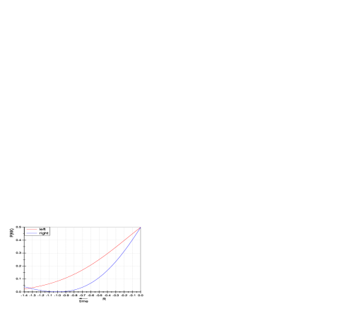
Figure 1: The comparison of QM prediction with the EI constraint. The horizontal axis refers to the values of R; vertical axis refers to the probabilities of corresponding events. The red line represents for the left side of inequality (9), and the blue for the sums of the right three terms.

Eberhard’s version of BI (EI) for kaon system takes the form [19, 20]:

$$P_{LR}(K^{0}\bar{K^{0}}) \leq P_{LR}(K^{0},K_{L})+P_{LR}(K_{S},K_{S})+P_{LR}(K_{L},\bar{K^{0}})\ ,$$ (9)

where $P_{\rm{LR}}$ denotes the LHVT transition probability with the subscripts L and R symbolling the left and right kaons, and we assume detection efficiency of the kaon decay products is one hundred per cent. For the case of QM, substituting equations (5) - (8) into the inequality (9) and assuming $\varphi=0$, we have

$$\frac{(2+\mathrm{R})^{2}}{4(2+\mathrm{R}^{2})} \leq \frac{(1+\mathrm{R})^{2}}{2(2+\mathrm{R}^{2})}\;+\;0\;+\;\frac{(1+\mathrm{R})^{2}}{2(2+\mathrm{R}^{2})}\ .$$ (10)

The above inequality is apparently violated by QM while $\mathrm{R}=-1$. The R dependence of the violation of inequality (10) is plotted in the Figure 1. Taking concurrence $C$ as a measure of entanglement [21] we have:

$$C(J/\Psi)=|\langle J/\Psi|\widetilde{J/\Psi}\rangle|=\frac{2}{2+|R|^{\,2}}=\frac{2}{2+|r|^{\,2}e^{(\Gamma_{S}-\Gamma_{L})\,T}}\ ,$$ (11)

where $|\widetilde{J/\Psi}\rangle=\sigma^{1}_{y}\sigma^{2}_{y}|(J/\Psi)^{*}\rangle\$ and $\sigma^{1,\ 2}$ are Pauli matrices. $C$ changes between null to unit for no entanglement and full entanglement. Superficially, equation (11) shows that the state become less entangled with the time evolution. However, our result, as shown in Figure 1, indicates clearly that there exists a period of time during which the violation of the inequality become larger with the time evolution. The larger violation for non-maximally entangled state than that of the maximally entangled state was also obtained by Acín et al. [22], where they use two d-dimensional ($d\geq 3$) quantum systems. To clarify this phenomenon we express the violation degree (VD) of the inequalities (left side subtract the right side) in term of $C$ and compare it with the usual CHSH inequality [23]. In Figure 2, the different VD behaviors of CHSH’s and Eberhard’s Inequalities are presented. For CHSH case, the $VD_{\rm CHSH}$ is obtained in the same condition as what the maximal violation happens in the full entanglement, the $C=1$. We have

$$VD_{CHSH}=\sqrt{2}(1+C)-2\ .$$ (12)

In fact, the above $VD_{\rm CHSH}$ can be deduced from the results given in Refs. [24, 25, 26]. For EI case, substituting Eq. (11) into (10) we have

$$VD_{EI}=\frac{-3(1-C)+2\sqrt{2}\sqrt{C-C^{2}}}{4}\ .$$ (13)

Here, in EI the counterintuitive quantum effect shows up, i.e. the less entanglement corresponding to a larger VD in some region, which is induced by the rotational symmetry breaking of the initial singlet state in quasi-spin space.

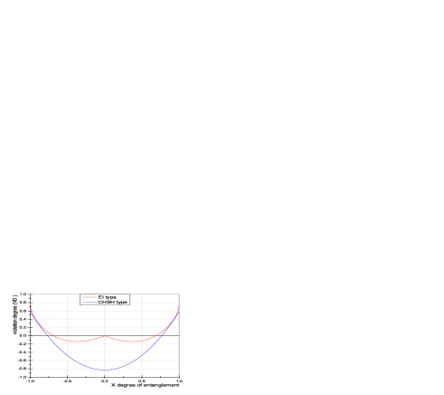
Figure 2: The violation degree of the Bell inequalities (red for EI type and blue for CHSH type) in terms of the entanglement. Here, for the sake of transparency, we make a coordinator exchange, the $C=1-x^{2}$. The magnitudes of VD less than zero means the broken of the BIs.

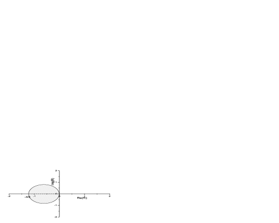
Figure 3: The practical complex $R$ values in distinguishing QM from LHVTs according to the inequality (9).

With the time evolution, when $R$ becomes less than $-\frac{4}{3}$, the QM and LHVTs both satisfy the inequality (9). Given a certain asymmetrically entangled state, the Hardy state [27], in the region of $R\in[-4/3,0)$ the QM and LHVTs can be distinguished from the EI. In preceding discussion, for simplicity we chose the phase of the complex quantity $R$ to be zero. However, in practice, the phase $\varphi$ can have a non-zero magnitude. Generally, as shown in Figure 3, the EI is violated by the QM in the shaded region of $R$.

To detect the $VD_{\rm EI}$, in experiment one needs to detect the decay events taking place between $T$ and $T+\Delta T$. Here, $T$ is the time when the entangled states are asymmetric and kept to be space-like in the follow up measuring interval $\Delta T$. In order to make sure the misidentification of $K_{S}$ and $K_{L}$ is less than one thousandth, the $\Delta\mathrm{T}$ should be larger than $5.5\tau_{S}$, which can be easily obtained, like

$$P_{survived}(K_{L}(\Delta T)) = \;|\,e^{-\frac{\Gamma_{L}}{2}\Delta T-im_{L}\Delta T}|^{\ 2}\;\simeq 99.0\%\ ,$$ (14)

$$P_{decayed}(K_{S}(\Delta T)) = 1-|\,e^{-\frac{\Gamma_{S}}{2}\Delta T-im_{S}\Delta T}|^{\ 2}\simeq 99.6\%\ .$$ (15)

In comparison with $\phi$ factory, the kaon system produced from the heavy Onium decay is easier to be space-like. The kaon pairs generated from $\phi$ decays moving at $\beta_{K}\simeq 0.22$. To ensure the entangled kaons to be space-like, the evolution time $T$ should larger than $11\tau_{S}$, which narrows the available region of $R$ in discriminating QM from LHVTs. In this case, the upper bound for $R$ is roughly

$$|R|=|r|e^{\frac{\Gamma_{S}}{2}T}\sim 0.4\ .$$ (16)

For kaons from $J/\Psi$ decay, $\beta_{K}=\frac{v_{K}}{c}\simeq 0.94$. This implies that as long as $T>(\beta^{-1}-1)\Delta\mathrm{T}/2\simeq 0.15\tau_{S}$ the space-like separation is guaranteed. Correspondingly, the $R$ is pretty small:

$$|R|=|r|e^{\frac{\Gamma_{S}}{2}T}\sim 10^{-3}\ .$$ (17)

This unique property of kaon system from Charmonium decays enables us to observe a peculiar QM effect, that is the less entangled state lead to a larger BI violation.

In conclusion, in this paper we propose to use the entangled kaon system produced in heavy quarkonium decay to test the LHVTs, that is the violation of a certain kind of Bell Inequality. We compare the difference in $\phi$ factory and quarkonium decays, and find that it is even possible to distinguish the Quantum Mechanics from the Local Hidden Variable Theories in the charmonium decays. In the charmonium decays the entangled kaon state is more energetic and easier to be space-like. On the other hand, in charmonium decays it is possible to observe a peculiar Quantum effect, that is the decreasing entanglement corresponds to the increasing BI violation in certain kinematic region. To be noticed that in order to have a unitary time evolution for the kaon system one has to include their decay states. This feature affects the Bell inequalities in certain degree, in particular the CHSH inequality [28], however, is not taken into account. In this work, we also give out the complete $R$ values for the BI violation in kaon system and express the violation in terms of degree of entanglement for the first time. Although the experimental efficiency for detecting the kaon system in heavy Onium decays is lower than the efficiency in $\phi$ factory, whereas our calculation shows that it is still possible to use $J/\Psi$ decay to kaons as a test of LHVTs in the future high statistic $\tau$-Charm factory. Moreover, it should be noted that our analyses and conclusions are generally also true for other heavy vector-like Onium decays.

This work was supported in part by the Nature Science Foundation of China and by the Scientific Research Fund of GUCAS(NO. 055101BM03). We are grateful to Z.P.Zheng, X.Y.Shan and H.B.Li for their helpful discussion.

References

- [1] A. Einstein, B. Podolsky and N. Rosen, Phys. Rev. 37, 777 (1935).
- [2] J.S. Bell, Phys. 1, 195 (1964).
-
[3]
A. Aspect, P. Grangier, and
G. Roger, Phys. Rev. Lett. 49, 91 (1982);
A.Aspect, J. Dalibard, and G. Roger, Phys. Rev. Lett. 49, 1804 (1982). - [4] P.R. Tapster, J.G. Rarity, and P.C.M. Owens, Phys. Rev. Lett. 73, 1923 (1994).
- [5] G. Weihs et al. Phys. Rev. Lett. 81, 5039 (1998).
- [6] D. Bohm, Y. Aharonov, Phys. Rev. 108, 1070 (1957).
- [7] M. Lamehi-Rachti, W. Mitting, Phys. Rev. D 14, 2543(1976).
- [8] S.A. Abel, M. Dittmar, and H. Dreiner, Phys. lett. B 280, 304 (1992).
- [9] H.J. Lipkin, Phys. rev. 176, 1715 (1968).
- [10] N.A. Törnqvist, Found. Phys. 11, 171 (1981).
- [11] P. Privitera, Phys. lett. B 275, 172 (1992).
- [12] A. Afriat, F. Selleri, The Einstein Podolsky and Rosen Paradox in atomic nuclear and particle physics. (Plenum Press, 1999).
- [13] Apollo. Go, Journal of Modern Optics 51, 991, (2004).
- [14] R.A. Bertlmann, A. Bramon, G. Garbarino, and B.C. Hiesmayr, Phys. lett. A 332, 355 (2004).
- [15] A. Bramon, G. Garbarino, Phys. Rev. Lett. 88, 040403 (2002).
- [16] J. Bernabéu, N. Mavromatos, and J. Papavassiliou, Phys. Rev. Lett. 92, 131601 (2004).
- [17] A. Bramon, G. Garbarino, Phys. Rev. Lett. 89, 160401 (2002).
- [18] A. Bramon, R. Escribano, and G. Garbarino, quant-ph/0501069.
- [19] P. Eberhard, Phys. Rev. A 47, R747 (1993).
- [20] A. Garuccio, Phys. Rev. A 52, 2535 (1995).
- [21] William K. Wootters, Phys. Rev. Lett. 80, 2245 (1998).
- [22] A. Acín, T. Durt, N. Gisin, and J.I. Latorre, Phys. Rev. A 65, 052325 (2002).
- [23] J.F. Clauser, M.A. Horne, A. Shimony, and R.A. Holt, Phys. Rev. Lett. 23, 880 (1969).
- [24] N. Gisin, Phys. Lett. A 154, 201 (1991).
- [25] G.Kar, Phys. Lett. A 204, 99 (1995).
- [26] Ayman F. Abouraddy, Bahaa E.A. Saleh, Alexander V. Sergienko, and Malvin C. Teich, Phys. Rev. A 64, 050101 (2001).
- [27] L. Hardy, Phys. Rev. Lett. 71, 1665 (1993).
- [28] R.A. Bertlmann and B.C. Hiesmayr, Phys. Rev. A63, 062112 (2001).