Dense-dilute factorization for a class of stochastic processes and for high energy QCD

Abstract

Stochastic processes described by evolution equations in the universality class of the FKPP equation may be approximately factorized into a linear stochastic part and a nonlinear deterministic part. We prove this factorization on a model with no spatial dimensions and we illustrate it numerically on a one-dimensional toy model that possesses some of the main features of high energy QCD evolution. We explain how this procedure may be applied to QCD amplitudes, by combining Salam’s Monte-Carlo implementation of the dipole model and a numerical solution of the Balitsky-Kovchegov equation.

I Introduction

High energy scattering in QCD was recently shown to be essentially similar to a reaction-diffusion process M2005 ; EGBM2005 . To understand this correspondence, one needs to introduce an (unphysical) forward elastic scattering amplitude $T(Y,r)$, that encodes the interaction probability for given parton or field configurations of the incoming hadrons, at rapidity $Y$, and for a characteristic transverse distance scale $r$. The physical scattering amplitude $A(Y,r)$ is the average of $T(Y,r)$ over all possible realizations of the fields or partons. Although $T$ is not measurable experimentally, it is a quantity that has also to be introduced when one wants to write a Monte-Carlo event generator.

The equation that governs the rapidity evolution of $T$ at fixed impact-parameter belongs to the universality class of the stochastic Fisher-Kolmogorov-Petrovsky-Piscounov (FKPP) equation FKPP , or equivalently, of the Reggeon field theory equation. It can be seen as a stochastic extension of the well-known Balitsky-Kovchegov (BK) equation B ; K , that describes a peculiar limit of high energy QCD. It is convenient to go to momentum space using the transformation K

$$\tilde{T}(Y,k)=\int\frac{d^{2}r}{2\pi r^{2}}e^{ikr}T(Y,r).$$ (1)

The evolution of $\tilde{T}$ can be written, for example, in the form

$$\partial_{\bar{\alpha}Y}\tilde{T}=\chi(-\partial_{\ln k^{2}})\tilde{T}-\tilde{T}^{2}+\alpha_{s}\sqrt{2\tilde{T}}\nu,$$ (2)

where $\bar{\alpha}=\alpha_{s}N_{c}/\pi$, $\chi$ is a representation of the BFKL kernel BFKL in momentum space and $\nu$ is a noise of zero mean that varies randomly by typically one unit when $\bar{\alpha}Y$ or $\ln k^{2}$ are changed by one unit. $\tilde{A}$ is the average of $\tilde{T}$ with respect to the noise $\nu$.

This new approach to high energy scattering in QCD, that makes use of ideas and tools of statistical physics, has already inspired a number of theoretical works. Eq. (2) itself was also subsequently discussed in Ref. IT2004 and studied numerically (with a Gaussian noise $\nu$) in Ref. S2005 . Many developments from different perspectives have followed: In particular, the connection to Reggeon field theory was investigated KovL2006 , a QCD derivation of Eq. (2) was searched for MSW2005 , and different formalisms to describe the same physics were proposed LL2005 .

Eq. (2) may be interpreted in the following way: It describes the evolution in time $t=\bar{\alpha}Y$ of a fraction $\tilde{T}$ of $N=1/\alpha_{s}^{2}$ particles (gluons) per unit of $x=\ln k^{2}$ that multiply and diffuse in $x$ through the branching diffusion kernel $\chi$, and that recombine through the nonlinear term. Eq. (2) is however not an exact equation of QCD, and should by no way be interpreted as such. It is rather a synthetic form of writing two exactly known limits: the large parton density limit, in which the evolution of $\tilde{T}$ is given by the Balitsky-Kovchegov equation

$$\partial_{\bar{\alpha}Y}\tilde{T}=\chi(-\partial_{\ln k^{2}})\tilde{T}-\tilde{T}^{2},$$ (3)

and the low density limit, represented by the linear stochastic equation

$$\partial_{\bar{\alpha}Y}\tilde{T}=\chi(-\partial_{\ln k^{2}})\tilde{T}+\alpha_{s}\sqrt{2\tilde{T}}\nu.$$ (4)

Let us briefly recall a bit more precisely the QCD content of Eq. (2) (We refer the reader to the original papers M2005 ; EGBM2005 for details). In the low density region of phase space (equivalently, in the region in which the amplitude is small, $T,\tilde{T}\ll 1$), it is useful to view rapidity evolution in the framework of the color dipole model M1993 . One goes to the reference frame of one of the interacting hadrons, that we assume to be a quark-antiquark dipole for simplicity and that we will call the probe. The second hadron carries all the rapidity and QCD evolution and will be referred to as the target. In the large-$N_{c}$ limit, the Fock state of the target may be represented by a set of color dipoles. Each of these dipoles, characterized by a two-dimensional position vector $x_{01}=x_{0}-x_{1}$ in transverse coordinate space, is spanned by two gluons respectively sitting at positions $x_{0}$ and $x_{1}$. The model is defined by the stochastic branching of the dipoles that occurs as the target is boosted to larger rapidities: In a step $dY$ of rapidity, each dipole present at rapidity $Y$ has the probability

$${\bar{\alpha}}dY\frac{d^{2}x_{2}}{2\pi}\frac{x_{01}^{2}}{x_{02}^{2}x_{12}^{2}}$$ (5)

to be replaced by two new dipoles of respective sizes $x_{02}$ and $x_{12}$.

When nonlinear effects can be neglected, the relationship between the number of dipoles $n(Y,x_{01})$ and the amplitude $T(Y,r_{01})$ for the scattering of the probe dipole of size $r_{01}$ off a random configuration of the target reads, in appropriate normalizations (see e.g. IM2003 ),

$$T(Y,r_{01})=\frac{\pi^{2}\alpha_{s}^{2}}{2}\\ \times\int\frac{d^{2}x_{0}}{2\pi}\frac{d^{2}x_{1}}{2\pi}\ln^{2}\frac{|r_{0}-x_{1}|^{2}|r_{1}-x_{0}|^{2}}{|r_{0}-x_{0}|^{2}|r_{1}-x_{1}|^{2}}n(Y,x_{01}).$$ (6)

This relationship turns out to be approximately local in dipole sizes and impact parameter: $T(Y,r_{01})$ is of order $\alpha_{s}^{2}$ times the number of dipoles in the considered configuration of the target whose sizes are in a bin of width 1 (on a logarithmic scale) centered on $|r_{01}|$, and which sit within a distance $|r_{01}|$ of the probe in impact parameter.

By converting the splitting process (5) into an evolution equation for $T$ with the help of Eq. (6), by transforming to momentum space using Eq. (1), and by averaging over the angle in the transverse plane, one would get the linear terms in Eq. (2) together with an appropriate noise $\nu$ that would encode the fluctuations in the dipole number induced by the stochastic branching process (5): this is precisely Eq. (4).

Dipole branching leads to an exponential increase of their number with rapidity, and consequently, to an unlimited rise of $T$ if formula (6) is applied: This would be inconsistent with unitarity, which requires the bound $T\leq 1$. It is believed that this rise is tamed by nonlinear effects GLRMQ that limit the number of dipoles in the target. Unfortunately, the latter effects have not yet been formulated in the framework of the dipole model. It is not even clear that dipoles should still be the relevant degrees of freedom in that regime.

On the other hand, one knows the equation that gives the average scattering amplitude at rapidity $Y+dY$ given the amplitude at rapidity $Y$, with the exact nonlinearity that preserves the unitarity of $T$. It reads:

$$\langle T(Y+dY,r_{01})|T(Y,r_{01})\rangle=T(Y,r_{01})+\\ \bar{\alpha}dY\int\frac{d^{2}r_{2}}{2\pi}\frac{r_{01}^{2}}{r_{02}^{2}r_{12}^{2}}(T(Y,r_{02})+T(Y,r_{12})-T(Y,r_{01})\\ -T(Y,r_{02})T(Y,r_{12})).$$ (7)

This equation is equivalent to the first equation in the celebrated Balitsky hierarchy B . Eq. (7) may be obtained from Eq. (2) by averaging it over the noise $\nu$ between rapidities $Y$ and $Y+dY$. A Fourier transformation to position space completes the identification. In practice, Eq. (7) is useful in a regime in which $T$ may be approximated by its average, i.e. when $\langle T(Y+dY,r_{01})|T(Y,r_{01})\rangle$ may be replaced by $T(Y+dY,r_{01})$, turning (7) into a closed equation for $T=\langle T\rangle$, Eq. (3). This is realized when the underlying effective number of dipoles is large, i.e. in the region of high density. The corresponding equation is the BK equation B ; K and is in the universality class of the (deterministic) FKPP equation MP2003 . The evolution of higher order correlators of $T$s that would be needed to be able to evolve $T$ also outside the dense region has still not been derived in a systematic way for the generic case of dipole-dipole scattering.

Although the correct formalism to describe the evolution of $T$ accurately in all regimes is still not available, exact asymptotic results BDMM2005 universal enough to also apply to QCD amplitudes have been found from the approximate formulation (2). Unfortunately, their validity is quite reduced since the limit $\ln(1/\alpha_{s}^{2})\gg 1$ had to be assumed, which is of course out of experimental reach. Hence it would be useful to understand what can be expected quantitatively from what is known up to now, beyond the far asymptotics.

The goal of this paper is to show that quite accurate results for the evolution of the QCD scattering amplitudes may be extracted from a numerical study that appropriately matches a Monte-Carlo simulation of the color dipole model, valid in the dilute regime, to the evolution of the amplitude given in Eq. (7), useful in the dense regime. We shall propose a factorization procedure of $T$, on an event-by-event basis, that we justify by a calculation in the framework of a zero-dimensional model and motivate and test on a one-dimensional toy model. We then explain how this factorization could be applied to QCD.

II Factorization in a zero-dimensional model

In a first stage, we study a zero-dimensional model (transverse variables are not considered) in order to introduce the factorization rigorously. Zero-dimensional models were investigated for possible applications to QCD some time ago M1994 ; Salam . Solutions for models of that kind have recently been discussed in Refs. SX2005 ; KL2006 , from different perspectives. The solutions which have been obtained will help us to assess the validity of the factorization that we shall propose here.

II.1 Definition of the model

We investigate the time evolution of a specific Markovian process in the universality class of the zero-dimensional stochastic FKPP equation. We consider a system of $n(t)$ particles. Between times $t$ and $t+dt$, each particle has a probability $p_{+}=dt$ to split in two particles. For each pair of particles, there is a probability $dt/N$ that one of them is lost, and thus each given particle has probability $p_{-}=(n_{t}-1)dt/N$ to disappear. These rules completely define the process.

There are several ways to represent this evolution. We may write the distribution of the number $n_{t+dt}$ of particles at time $t+dt$ given the number of particles $n_{t}$ at time $t$:

$$P(n_{t+dt}|n_{t})=\delta_{n_{t+dt},n_{t}}\left(1-n_{t}dt-\frac{n_{t}(n_{t}-1)}{N}dt\right)\\ +\delta_{n_{t+dt},n_{t}+1}n_{t}dt+\delta_{n_{t+dt},n_{t}-1}\frac{n_{t}(n_{t}-1)}{N}dt.$$ (8)

This equation may be cast in the form of a stochastic equation for $n_{t}$ by first computing the mean and variance of $n_{t+dt}$ given $n_{t}$, with the help of Eq. (8). This enables one to write the time evolution of $n_{t}$ in terms of a drift and of a noise of zero-mean and normalized variance, namely:

$$\frac{dn_{t}}{dt}=n_{t}-\frac{n_{t}(n_{t}-1)}{N}+\sqrt{n_{t}+\frac{n_{t}(n_{t}-1)}{N}}\nu_{t+dt},$$ (9)

where $\nu$ is such that $\langle\nu_{t}\rangle=0$ and $\langle\nu_{t}\nu_{t^{\prime}}\rangle=\delta(t-t^{\prime})$. Note that the distribution of $\nu$ depends on $n_{t}$ and is not a Gaussian. This last point is easy to understand: The evolution of $\nu_{t}$ is intrinsically discontinuous, since it stems from a rescaling of $n_{t}$, which is an integer at all times. A Brownian evolution (i.e. with a Gaussian noise) would necessarily be continuous. For completeness, we write the statistics of $\nu_{t+dt}$, which is easy to derive from the evolution of $n$:

$$\nu_{t+dt}=\begin{cases}\phantom{-}\frac{1}{\sigma\,dt}-\frac{\Delta}{\sigma}&\text{proba}\ {n_{t}\,dt}\\ \phantom{-\frac{1}{\sigma\,dt}}-\frac{\Delta}{\sigma}&\text{proba}\ 1-n_{t}\,dt-\frac{n_{t}(n_{t}-1)}{N}dt\\ -\frac{1}{\sigma\,dt}-\frac{\Delta}{\sigma}&\text{proba}\ \frac{n_{t}(n_{t}-1)}{N}dt,\end{cases}$$ (10)

where $\Delta=n_{t}-\frac{n_{t}(n_{t}-1)}{N}$ and $\sigma=\sqrt{n_{t}+\frac{n_{t}(n_{t}-1)}{N}}$. We see well the jumps induced by the terms proportional to $1/dt$.

Formulating the process with the help of a stochastic equation such as (9) has no real advantage at this point. Here, we just aimed at showing explicitely the connection with stochastic partial differential equations.

II.2 Poissonian states and “Pomerons”

Instead of looking at a state of definite occupancy, one could also consider the evolution of a Poissonian state whose occupation numbers are distributed as

$$P_{z_{t}}(n_{t})=\frac{z_{t}^{n_{t}}}{n_{t}!}e^{-z_{t}}$$ (11)

and follow the evolution of $z_{t}$, that is to say, compute the probability distribution of $z_{t+dt}$ given $z_{t}$, $P(z_{t+dt}|z_{t})$. As can be easily checked, the moments of $z_{t+dt}$ are the factorial moments of $n_{t+dt}$. This statement may be written as

$$\sum_{n_{t},n_{t+dt}}\frac{n_{t+dt}!}{(n_{t+dt}-k)!}P(n_{t+dt}|n_{t})P_{z_{t}}(n_{t})\\ =\int dz_{t+dt}z_{t+dt}^{k}P(z_{t+dt}|z_{t}).$$ (12)

Replacing Eqs. (8) and (11) in Eq. (12), one finds

$$\int dz_{t+dt}z_{t+dt}^{k}P(z_{t+dt}|z_{t})=z_{t}^{k}+dt\left[z_{t}-\frac{z_{t}^{2}}{N}\right]kz_{t}^{k-1}\\ +\frac{1}{2}\left[{2dt}\left(z_{t}-\frac{z_{t}^{2}}{N}\right)\right]k(k-1)z_{t}^{k-2},$$ (13)

from which it is obvious that $P(z_{t+dt}|z_{t})$ is a Gaussian of mean $z_{t}+dt(z_{t}-\frac{z_{t}^{2}}{N})$ and variance ${2}{dt}{(z_{t}-\frac{z_{t}^{2}}{N})}$. In the same way as one translates Eq. (8) into Eq. (9), this may be expressed in the form of a stochastic evolution equation for $z_{t}$ PL

$$\frac{dz_{t}}{dt}=z_{t}-\frac{z_{t}^{2}}{N}+\sqrt{2\left(z_{t}-\frac{z_{t}^{2}}{N}\right)}\eta_{t+dt}.$$ (14)

This is an Ito equation: $\eta$ is a Gaussian white noise satisfying $\langle\eta_{t}\rangle=0$ and $\langle\eta_{t}\eta_{t^{\prime}}\rangle=\delta(t-t^{\prime})$. $z_{t}$ is now evolving continuously, unlike $n_{t}$. Eq. (14) is the zero-dimensional version of the stochastic FKPP equation. It is of course consistent with Eq. (9), since the moments of $z$ are the factorial moments of $n$. Starting from Eq. (14) and transforming it into a hierarchy for the factorial moments of $n_{t}$, one can compute the first few orders of $\langle n_{t}\rangle$ in a $1/N$ expansion resummed for large $t$ SX2005 . The result turns out to be an asymptotic Borel-summable series. It reads M1994 ; SX2005

$$\langle n_{t}\rangle=N\sum_{k=1}^{\infty}(-1)^{k+1}{N}^{-k}k!e^{kt}.$$ (15)

Each term may be interpreted as the result of the evaluation of a diagram with a number $k$ of “Pomerons” being exchanged in the $t$-channel. We refer the reader to SX2005 for a detailed calculation in such a framework.

The series (15) can be rewritten in the form of a Borel integral,

$$\langle n_{t}\rangle=N\left(1-Ne^{-t}\int^{\infty}_{0}\frac{db}{1+b}e^{-Ne^{-t}b}\right),$$ (16)

which eventually may be expressed in terms of special functions.

Eqs. (15) and  (16) are a priori valid for $e^{t}/N\ll 1$. Actually, it was found in Ref. SX2005 from the exact evaluation of subleading orders, that its effective range of validity is much broader, $t/N\ll 1$.

The classical limit is also easily identified from Eq. (14): Indeed, a classical state has a definite value of $z$. The classical path $z(t)=\langle n_{t}\rangle\simeq n_{t}^{\text{MF}}$ is obtained by solving the deterministic part of Eq. (14), namely

$$\frac{dn^{\text{MF}}_{t}}{dt}=n^{\text{MF}}_{t}-\frac{(n^{\text{MF}}_{t})^{2}}{N}.$$ (17)

This approximation is expected to be valid only when the typical number of particles in the system is large. It is useful to notice that the steady fixed point of the evolution is $\langle n_{t}\rangle=N$.

The formulation of Eq. (14) is helpful for analytical calculations of the moments of $n_{t}$. However, in order to describe a physical system that starts evolution with a definite number of particles, one needs to introduce complex values of the Poisson parameter $z$. This makes Eq. (14) of little interest for numerical simulations of such systems. Furthermore, the analytical method for the computation of moments is very awkward to transpose numerically, since it leads to an asymptotic series that eventually needs to be resummed. Finally, it is not straightforward to generalize to models with spatial dimensions.

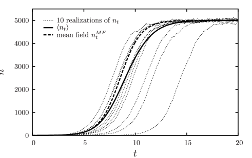
Figure 1: Bunch of dotted lines: Ten different paths for $n_{t}$ obtained from the evolution (9) of the zero-dimensional model starting from a single-particle initial condition. Dashed line: Mean-field solution, see Eqs. (17),(20). Full line: Numerical solution for $\langle n_{t}\rangle$ obtained by averaging over a large number of realizations of Eq. (9).

II.3 Solving the stochastic evolution for $n$: dense-dilute factorization

For the difficulties mentioned above with the Poissonian state approach, we wish to take a different point of view on the evolution of the stochastic model. Instead of performing a large-$N$ perturbative calculation directly of $\langle n_{t}\rangle$ using field-theoretical methods, we try to characterize the shape of each realization of an evolution that starts with $n_{0}=1$ particles. What we mean by “realization” is a given path for $n$ generated by the stochastic evolution (9).

It is useful to visualize a few such realizations: This is shown in Fig. 1 for $N=5000$, together with the solution to the mean field equation (17). One sees that the curves that represent $n_{t}$ look like the solution to the mean-field equation (17), but with the origin of times translated by some random $t_{0}$. (The curves look also slightly noisy around the average trend, but the noise would be still much weaker for larger values of $N$). This suggests that once there are “enough” particles in the system, say $\bar{n}\gg 1$, the evolution becomes essentially deterministic. Hence stochasticity only manifests itself in the initial stages of the evolution until $n_{t}=\bar{n}$, but in a crucial way: Indeed, as seen in Fig. 1, after averaging, $\langle n_{t}\rangle$ is significantly different from $n_{t}^{\text{MF}}$, and this difference stems from rare realizations in which the particle number stays low for a long time. Therefore, in individual realizations, stochasticity should be taken into account exactly as long as $n_{t}<\bar{n}$. Fortunately, when the number of particles in the system is small compared to the maximum number of particles $N$, the stochastic evolution is essentially governed by a linear equation which is not difficult to handle analytically.

This heuristical discussion suggests that we may factorize the evolution in a linear stochastic evolution up to the time at which the number $n$ of particles in the system reaches $\bar{n}$, and continue through a nonlinear but deterministic equation, which is obtained from a mean field approximation to the evolution equation. As we will see, this simple observation leads to an elegant computation of $\langle n_{t}\rangle$ that consistently agrees with the lowest order (see Eq. (16)) derived in Ref. M1994 ; SX2005 .

Let us denote by $p_{\bar{n}}(\bar{t})$ the distribution of the times at which the number of particles in the system reaches $\bar{n}$ and $\langle n_{t}|n_{\bar{t}}\rangle$ the conditional average number of particles at time $t$ given that there are $n_{\bar{t}}$ particles in the system at time $\bar{t}$. One may write

$$\langle n_{t}\rangle=\int_{0}^{\infty}d\bar{t}\,p_{\bar{n}}(\bar{t})\langle n_{t}|n_{\bar{t}}\rangle.$$ (18)

So far, this expression is exact.

We now assume that the evolution is linear when $n_{t}<\bar{n}$ and deterministic for $n_{t}>\bar{n}$. Thus, in the previous equation, we replace $p_{\bar{n}}(\bar{t})$ by the solution $p_{\bar{n}}^{\text{lin}}(\bar{t})$ of the linear problem obtained by setting $p_{+}=dt$ and $p_{-}=0$. Furthermore, we approximate $\langle n_{t}|n_{\bar{t}}\rangle$ by the solution to the nonlinear evolution in the mean field approximation (17) over a time interval $t-\bar{t}$ starting with $\bar{n}$ particles at time $\bar{t}$, that we denote by $n^{\text{MF}}_{t-\bar{t}|\bar{n}}$ . In these notations, we find the factorization

$$\langle n_{t}\rangle=\int_{0}^{\infty}d\bar{t}\,p^{\text{lin}}_{\bar{n}}(\bar{t})n^{\text{MF}}_{t-\bar{t}|\bar{n}}.$$ (19)

Note that for $\bar{t}>t$ (i.e. when there are less than $\bar{n}$ particles in the system at the considered time $t$), $n^{\text{MF}}_{t-\bar{t}|\bar{n}}$ is like a backward evolution towards lower number of particles. This is not a problem since we then go back to the dilute regime, and the solution for $\langle n\rangle$ in that regime is just obtained by taking the dilute limit of $n^{\text{MF}}$, given by the solution of the equation obtained from Eq. (17) by dropping the nonlinear term.

We claim that this factorization is valid whenever $\bar{n}$ is large enough compared to 1 to justify the mean field approximation for the subsequent evolution, but, at the same time, $\bar{n}$ is small compared to $N$ in such a way that the evolution up to $\bar{n}$ be linear.

Let us express give explicit expressions for the different quantities that appear in Eq. (19). The solution to Eq. (17) reads

$$n^{\text{MF}}_{t-\bar{t}|\bar{n}}=\frac{N}{1+\frac{N}{\bar{n}}e^{-(t-\bar{t})}}$$ (20)

for $\bar{n}\ll N$. It is also not difficult to show that $p_{\bar{n}}^{\text{lin}}$ solves the equation

$$p^{\text{lin}}_{\bar{n}}(\bar{t})=(\bar{n}-1)\int_{0}^{\bar{t}}d{\bar{t}}^{\prime}\,p^{\text{lin}}_{\bar{n}-1}({\bar{t}}^{\prime})e^{-(\bar{n}-1)({\bar{t}}-{\bar{t}}^{\prime})}.$$ (21)

Its solution may be found by standard generating function methods and takes the simple form

$$p^{\text{lin}}_{\bar{n}}({\bar{t}})=(\bar{n}-1)e^{-{\bar{t}}}(1-e^{-{\bar{t}}})^{\bar{n}-2}.$$ (22)

In the limit of interest, that is for large $\bar{n}$ and $\bar{t}$, it boils down to a Gumbel distribution

$$p^{\text{lin}}_{\bar{n}}({\bar{t}})=\bar{n}e^{-{\bar{t}}-\bar{n}e^{-{\bar{t}}}}.$$ (23)

Replacing Eqs. (20) and (23) in Eq. (19), we find

$$\langle n_{t}\rangle=N\int_{0}^{\infty}d\bar{t}\,\frac{\bar{n}e^{-\bar{t}-\bar{n}e^{-\bar{t}}}}{1+\frac{N}{\bar{n}}e^{-(t-\bar{t})}}.$$ (24)

Since the Gumbel distribution is strongly damped for $\bar{t}<0$ (by a factor $e^{-\bar{n}}$), we may safely replace the lower limit of the integral by $-\infty$. Finally, the change of variable $b=\frac{\bar{n}}{N}e^{t-\bar{t}}$ brings the integral in the form (16). The result is independent of $\bar{n}$, as it should be, but in numerical applications, one should keep in mind that the limits $1\ll\bar{n}\ll N$ have been assumed, and thus finite $\bar{n}$ corrections must be expected.

In this picture, the Borel integral (16) has a transparent interpretation: the parameter $b$ is related to the factorization time $\bar{t}$, the exponential is the distribution of $\bar{t}$ and the denominator corresponds to the mean-field part. Our method allowed to directly arrive at the leading order result found in Refs. M1994 ; SX2005 , without having to resum an asymptotic (divergent) series.

III A one-dimensional toy model

We shall now formulate and test this dense-dilute factorization on a one-dimensional toy model. Again, we consider a system made of typically $N$ particles in its steady state.

With one space dimension labeled by the real variable $x$, for large enough times, the particles form a front that travels towards say larger values of $x$ when time flows PVS ; EGBM2005 . Its position $X_{t}$ may be taken as the position of the $(N/2)$-th rightmost particle. This front connects a dilute region, to the right, to a denser region to the left. There is a point in the front around which the typical number of objects is $\bar{n}$. In the spirit of the previous section, we will treat the evolution to the right of this point as stochastic and solve a mean field equation to the left. We will explain the factorization and illustrate it numerically on a specific particle model that was introduced in Ref. BDMM2006 .

When one takes a new step in time $t\rightarrow t+\Delta t$, the particle at position $x_{i}(t)$ is replaced, with probability $\Delta t$, by two particles at positions, where $\delta_{1}$ and $\delta_{2}$ are distributed according to $\psi(\delta_{1})d\delta_{1}$ (resp. $\psi(\delta_{2})d\delta_{2}$). This rule defines the evolution of the number of particles in a way analogous to the dipole splitting rule in QCD. To implement a simple form of saturation of the number of particles, only the $N$ particles which have largest positions are kept for subsequent evolution.

We define $T(t,x)$ as the fraction of these $N$ particles that have positions larger than $x$ at time $t$, that is

$$T(t,x)=\frac{1}{N}\sum_{i=1}^{N}\Theta(x_{i}(t)-x).$$ (25)

Obviously, $T(t,-\infty)=1$ and $T(t,+\infty)=0$ for $t$ large enough for the total number of particles in the system to have reached $N$.

Considering for a while the $N=\infty$ limit, the mean evolution of $T$ in one elementary step in time reads

$$\langle T(t\!+\!\Delta t,x)|T(t,x)\rangle\\ =\min\left(1,(1-\Delta t)T(t,x)+2\Delta t\int d\delta\,\psi(\delta)T(t,x-\delta)\right).$$ (26)

This equation is the analogous of the first equation in the Balitsky hierarchy in the QCD case, see Eq. (7). In the infinite $N$ limit, it is known that the large time solutions are traveling waves whose average velocity is determined by the linearized part of Eq. (26). If one defines

$$v(\gamma)=\frac{1}{\Delta t}\frac{1}{\gamma}\ln\left(1-\Delta t+2\Delta t\int d\delta\,e^{\gamma\delta}\psi(\delta)\right),$$ (27)

then $v(\gamma)$ admits a minimum at $\gamma=\gamma_{0}$ and the large-time front velocity is $v(\gamma_{0})$. At finite $N$, the position of the front becomes stochastic, with nontrivial (non-Gaussian) statistics. The moments of the position of the front are known for large $N$ BDMM2005 . The first two of them read

$$V\times t\equiv \langle X_{t}\rangle=v(\gamma_{0})t-\frac{\pi^{2}\gamma_{0}^{2}v^{\prime\prime}(\gamma_{0})}{2\ln^{2}N}t,$$ (28a)

$$D\times t\equiv \langle X_{t}^{2}\rangle-\langle X_{t}\rangle^{2}=\frac{\pi^{4}\gamma_{0}v^{\prime\prime}(\gamma_{0})}{3\ln^{3}N}t.$$ (28b)

The average position of the front was first obtained by considering a deterministic evolution equation with a cutoff BD ; MS2004 that simulates the discreteness of the particles in the system BD . In our case, one would write

$$T^{\text{cutoff}}(t\!+\!\Delta t,x)=\min\bigg{(}1,(1-\Delta t)T^{\text{cutoff}}(t,x)\\ +2\Delta t\int d\delta\,\psi(\delta)T^{\text{cutoff}}(t,x-\delta)\bigg{)}\\ \times\Theta[T^{\text{cutoff}}(t+\Delta t,x)-{{1}/{N}}].$$ (29)

The first correction to this approximation (not shown in Eq. (28a)) is also known BDMM2005 . It is due to particles that are randomly sent ahead of the deterministic part of the front (to the left of the cutoff), at some distance to the right of the tip of the front. Their multiplication through time evolution pulls the front forward, and generates a positive correction to the velocity and the dispersion in the front position $D$ given in Eq. (28b). One also knows that the system is completely renewed every $t\sim 1/D$ units of time BDMM2006 . This remark will help the analysis of the numerical data.

In our numerical implementation, we choose $\psi$ to be the uniform distribution in the interval $[0,1]$, i.e.

$$\psi(\delta)=\Theta(\delta)\Theta(1-\delta),$$ (30)

and $\Delta t=0.1$. Solving $v^{\prime}(\gamma_{0})=0$ where $v(\gamma)$ is given by Eq. (27) with these settings, we get

$$\begin{split}\gamma_{0}&=1.46256\cdots,\\ v(\gamma_{0})&=2.07006\cdots,\\ v^{\prime\prime}(\gamma_{0})&=0.753472\cdots.\end{split}$$ (31)

$\gamma_{0}$ is the logarithmic slope of the falloff of the front. $v(\gamma_{0})$ is the velocity in the $N=\infty$ limit. $v^{\prime\prime}(\gamma_{0})$ is a parameter that appears when one considers finite-$N$ corrections.

We first solve the complete stochastic model. We take an initial condition of the form $x_{1}=\cdots=x_{N}=0$ (that is $T(t=0,x)=\Theta(-x)$) and evolve it in time using the exact evolution rules. We evolve the system over $p\times 500$ units in $t$ ($p$ is 500 in our simulation), recording the position of the front $X_{t_{i}}$ every $\delta t=t_{i}-t_{i-1}=500$ units of time. We compute $V=\langle\delta_{i}X_{t}\rangle/\delta t$, where $\delta_{i}X_{t}=X_{t_{i}}-X_{t_{i-1}}$, and $D=(\langle\delta_{i}X_{t}^{2}\rangle-\langle\delta_{i}X_{t}\rangle^{2})/\delta t$. The average is over the $p$ periods of $\delta t$ units of time in one single realization, but for an ergodic system, averaging over the time evolution of one realization is like averaging over many independent realizations of the evolution.

Since the system renews itself every $1/D$ units of time, and since $1/D$ is at most of order 100, the differences of successive positions $\delta_{i}X_{t}$ are essentially independent random variables. Hence we can estimate the statistical uncertainties by splitting our set of positions $\delta_{i}X_{t}$ in say 10 subsets, and by evaluating the dispersion of $V$ and $D$ between these different subsets. This helps us to provide error bars. The results are shown in Tab. 1 and in Figs. 2 and 3 for $N=10^{2},10^{3},10^{4},10^{5}$.

We also solve the deterministic evolution with a cutoff, defined in Eq. (29). To this aim, we need to take a discretization in the $x$ variable: We define a lattice with 1000 points per unit of $x$. The integration over $\delta$ in Eq. (29) is performed using the rectangle method. Although this method converges very slowly (one expects a systematic error of the order of $0.1\%$ in our settings), it is quite well suited here because as we impose a cutoff at each step of the evolution, $T^{\text{cutoff}}$ has sharp discontinuities. The result is shown in Fig. 2 together with the theoretical formula (28a), with which there is a very good agreement except for the lowest values of $N$. But that is expected since Eq. (28a) was obtained in a large-$N$ limit of the deterministic evolution with a cutoff. The slight discrepancy (of order $0.1\%$) visible at large $N$ is consistently explained by the fact that our discretization and our integration method amount to solving a model on a lattice rather than the original model in the continuum, for which one can compute the asymptotic front velocity $v(\gamma_{0})$, which is indeed slightly lower.

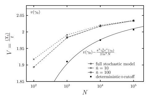
Figure 2: Average velocity of the front $V$ versus the equilibrium number of particles $N$ for the toy model. The full curves represent theoretical estimates. The black squares is the result of the mean-field calculation with a cutoff. The solution of the full stochastic model is shown with circles linked by large dashed lines. The solution of the mixed method for $\bar{n}=10$ is displayed with crosses linked by short dashed lines. White squares denote the case $\bar{n}=100$, but they are almost indistinguishable from the solution of the full stochastic model.

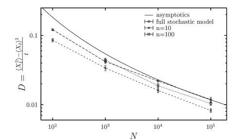
Figure 3: Diffusion coefficient of the front $D$ versus $N$. Same legend as in Fig. 2.

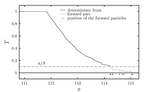
Figure 4: One realization of the front for $N=100$ evolved using the mixed method with a factorization scale $\bar{n}=10$. Below $x_{\text{m}}$, the front is represented by $T$ evolved deterministically. For $x>x_{\text{m}}$, the position of each particle is recorded and evolved using the exact stochastic rules.

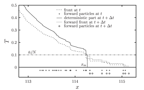
Figure 5: One realization of the evolution of the front of Fig. 4 (reproduced here in dashes) over the time interval $\Delta t$. The backward part is evolved through Eq. (26) (full line). The crosses mark the positions of the particles that are used as an input for the stochastic evolution of the forward tail (they include the particles represented in Fig. 4 whose positions are tracked exactly, and additional particles generated from $T$). The circles denote the particles that are kept at time $t+\Delta t$: most of them were already present at $t$, and two of them have been produced stochastically. The forward part of $T$ at time $t+\Delta t$ is represented in short dashes.

Next, we perform a mixed evolution, applying our dense-dilute factorization procedure. This goes as follows. At all times, the forward part of the front where $T(t,x)\leq\bar{n}/N$ is represented by the positions of the $\bar{n}$ foremost particles, and the latter are evolved using the exact rule (we must drop the nonlinearity, but for this model it only amounts to selecting the $N$ most forward particles: If $\bar{n}$ is small enough, the forward particles alone cannot have more than $N$ offsprings in one iteration). This is illustrated in Fig. 4 for a particular realization and for a particular choice of the parameters $N$ and $\bar{n}$. For $T(t,x)>\bar{n}/N$, we directly evolve $T$ using Eq. (26) with the approximation $\langle T(t\!+\!\Delta t,x)|T(t,x)\rangle=T(t\!+\!\Delta t,x)$, forgetting about the exact position of each individual particle. More technically, an evolution over the time interval $\Delta t$ goes as follows. We first generate particle positions from $T$ in the region of $x$ between $x_{\bar{n}}-1$ and $x_{\bar{n}}$. Indeed, in our model, it is precisely the particles present in that interval that may split into the forward region where we decided to keep the full stochasticity. This is related to our particular choice of $\psi$, see Eq. (30), but in practice, it is enough that the splittings be local enough in $x$. This is indeed the case for the fixed impact parameter BFKL evolution in QCD (see Eq. (2) with $x=\ln k^{2}$). To get back the particle positions from the profile of $T$ is extremely straightforward in this particular model: the position $x_{i}$ of particle number $i$ is the rightmost point for which $T(t,x_{i})=i/N$ holds (In more subtle models such as QCD, one would have to invert a relation like Eq. (6)). The positions of the obtained particles are shown with crosses in Fig. 5. We then evolve these additional particles together with the $\bar{n}$ forward particles using the full stochastic rule. Simultaneously, we evolve $T$ deterministically for all $x$, but we cut the result at $x_{\text{m}}$ defined as the position in the front for which $T(t+\Delta t,x_{\text{m}})=\bar{n}/N$. Indeed, only for $T>\bar{n}/N$ do we trust the mean-field approximation $\langle T(t\!+\!\Delta t,x)|T(t,x)\rangle=T(t\!+\!\Delta t,x)$. In turn, we only keep the forward particles that have positions larger than $x_{\text{m}}$. Finally, the matching of the forward and backward parts of the front is done by requiring that $T$ be a decreasing function of $x$. In the case in which there is a number of particles larger than $\bar{n}$ produced ahead of $x_{\text{m}}$, then $T$ computed from the forward particles is larger than $\bar{n}/N$ at $x_{\text{m}}$: We choose to continue $T(t+\Delta t,x_{\text{m}})$ for $x<x_{\text{m}}$ until the point at which $T(t+\Delta t,x)=T(t+\Delta t,x_{\text{m}})$. Note that with this prescription for the matching, the particle distribution in the forward part of the front is exact at all times, but the number of particles in the backward part is slightly overestimated on the average. Other prescriptions may have been chosen: They would lead to similar quantitative results. One particular realization of the resulting front is shown in Fig. 5.

We turn to the discussion of the numerical results for the mixed method. Recall that the factorization scale $\bar{n}$ has to be at the same time larger than 1 in such a way that mean field evolution starting from $\bar{n}$ can be justified, and much smaller than $N$ so that nonlinear effects may be neglected. We choose $\bar{n}=10$ and $\bar{n}=100$. This means that the minimum value of $N$ for which we may solve the model using our method is of the order of $100$ for $\bar{n}=10$ and $1000$ for $\bar{n}=100$. We follow exactly the same procedure as in the fully stochastic case: We evolve the same initial condition over $p\times 500$ steps of time, with $p=500$.

The calculations of the velocity of the front are presented in Tab. 1. In Fig. 2, they are compared to the results obtained by solving the exact model. We observe a perfect agreement for $\bar{n}=100$, at the level of $0.1\%$. For $\bar{n}=10$, the agreement is less good: the velocity is overestimated by about $1\%$ (but this means a $10\%$ mismatch in the difference $v(\gamma_{0})-V$ with the infinite-$N$ velocity). Of course, a better agreement than that could not really be expected. However, part of the mismatch may also be related to the fact that our matching prescription between the dense and dilute regions leads to a slight overestimate of the number of particles in the lower part of the dense region, which has indeed the effect of increasing the front velocity. It may well be that for different models which do not have the requirement that $T$ be a decreasing function of $x$, like QCD, the agreement would even be better.

The diffusion coefficient $D$ of the front is given in Tab. 1 and displayed in Fig. 3. We also plot the theoretical formula (28b), to guide the eye. The numerical data seem to agree well with the asymptotic theoretical estimate (28b), but this must be accidental since for the considered values of $N$, corrections are expected to be huge. The diffusion coefficient is a quantity that is much more difficult to measure numerically than the velocity, since it requires more statistics. Our error bars are still of the order of 5 to 10%. We see however that the full stochastic model is very well reproduced, within errors, by the mixed model with $\bar{n}=100$. For $\bar{n}=10$ instead, we notice that the fluctuations seem to be globally underestimated by up to 30% (see Tab. 1). But this should be expected since our method consists in replacing part of the stochastic evolution by a mean field approximation.

	$N$	stochastic	$\bar{n}=10$	$\bar{n}=100$
$V$	$10^{2}$	$1.8937(3)$	$1.9173(5)$	—
	$10^{3}$	$1.9824(2)$	$1.9910(2)$	$1.9838(4)$
	$10^{4}$	$2.0176(2)$	$2.0202(3)$	$2.0173(3)$
	$10^{5}$	$2.0348(2)$	$2.0345(2)$	$2.0331(2)$
$D$	$10^{2}$	$121.2\pm 3.9$	$85.47\pm 4.51$	—
$\times 10^{3}$	$10^{3}$	$41.87\pm 2.46$	$33.89\pm 2.96$	$44.19\pm 2.74$
	$10^{4}$	$21.99\pm 0.68$	$16.07\pm 1.21$	$18.73\pm 1.36$
	$10^{5}$	$11.82\pm 0.93$	$8.243\pm 0.498$	$10.38\pm 0.68$

Table 1: Numerical results for the one-dimensional toy model. The velocity $V$ and the diffusion coefficient $D$ of the front are computed in the full stochastic model and in the two mixed models with factorization scales $\bar{n}=10$ and $\bar{n}=100$ respectively, for four different values of $N$.

IV Outlook for QCD

We have worked on specific toy models of noisy evolution of the FKPP type. We have proposed that, on an event-by-event basis, their evolution may be factorized into a linear stochastic part and a nonlinear deterministic part. We have shown on a zero-dimensional model that writing down this factorization leads to a straightforward computation of the average number of particles at leading order in $t/N$, without having to go through the resummation of a divergent series like in more standard approaches M1994 ; Salam ; SX2005 .

We have conjectured that such a factorization is also valid for one-dimensional models. In fact, this factorization had already been implicitly assumed in previous works in statistical physics, essentially for the purpose of performing numerical calculations for very large values of $N$ BD ; Moro ; EGBM2005 . In Ref. BDMM2005 , it was even used to obtain analytical results for the front position, but only exponentially large values of $N$ were attainable. We have shown here that this factorization may be extended (in practice numerically) to lower values of $N$, of the order of $100$ or $1000$. The only condition is the existence of a mesoscopic scale of particle numbers $\bar{n}$ such that $1\ll\bar{n}\ll N$. We have tested the factorization in a model that we could also solve numerically, and have shown that it reproduces quite well the exact solution even for values of $N$ as low as 100.

Of course, the dense-dilute factorization would be of no interest for numerical calculations at low values of $N$ in cases in which the complete underlying stochastic model were known – systems with 100 or 1000 particles may often be simulated quite easily. However, as we have recalled in the introduction, the exact formulation of high energy QCD as a stochastic process (if it exists) has not been found yet. Instead, we have a probabilistic rule for the evolution of the dipole number $n$ valid in the dilute regime of small amplitudes (see Eq. (5)), which has already been implemented numerically by Salam Salam (see also A2004 ), and a mean-field equation for evolving the amplitude $T$ in the dense regime (the Balitsky-Kovchegov equation B ; K , see Eq. (7)). In our toy model, the latter is equivalent to Eq. (26) and the former is like the evolution rule for our system of particles. In addition, the relationship between $n$ and $T$ in the dilute regime is needed: it is provided by Eq. (6) in QCD, and has its equivalent (Eq. (25)) in the toy model of the previous section. Consequently, the factorization proposed here should be very well suited for numerical computations of QCD scattering amplitudes at high energy: One should combine Salam’s dipole Monte-Carlo and a solution of the Balitsky-Kovchegov equation, in a way similar to what we have done here for the one-dimensional toy model. The details will be worked out in another publication IMMS .

Extrapolating the results of our toy model study, we can expect to get reliable results for models in which the typical allowed number of particles $N$ is larger than $100$. This corresponds to $\alpha_{s}<0.1$ in QCD, which is not far from the experimentally accessible window. Hence the factorization procedure outlined here may be a good starting point for a realistic numerical investigation of QCD amplitudes near the unitarity limit. Anyway, it is probably the best one could achieve without finding a realization of nonlinear saturation effects in the dipole model. Needless to say, the toy model that we have studied here was tuned to make our factorization procedure as easy as possible to handle numerically. The many complications of QCD will make the implementation of this factorization a challenging issue.

At a more theoretical level, what our study suggests is that universal features show up already for quite low values of $N$. This leaves us with the hope that the asymptotic analytical calculations of Ref. BDMM2005 could be extended to a wider range in $N$.

Finally, we wish to comment on a recent proposal on how to address numerically the problem of QCD evolution at very high energies beyond the mean-field BK limit. In Ref. KL , the idea that fluctuations could be obtained by solving a classical equation and then averaging over an ensemble of initial conditions was suggested, and was implemented numerically subsequently in Ref. AM . We note that the philosophy of this proposal is orthogonal to the one developed here: In our view, fluctuations in the saturation scale are due to intrinsic noise related to the discreteness of the number of partons, as is natural in reaction-diffusion processes. We do not think that the approach of Refs. KL ; AM would work for reaction-diffusion at very large times (i.e. asymptotic energies): For example, a universal distinctive feature of such processes is that the dispersion of the front positions (i.e. saturation scales) between different realizations (i.e. events) scales like $\sqrt{Y}$, which cannot be reproduced in the approach of Refs. KL ; AM . Since our numerical method relies on the conjecture that QCD evolution is in the same universality class as reaction-diffusion processes, the two approaches would not lead to the same results for QCD observables (see Ref. AM ). However, since the statement that there is a correspondence between QCD and reaction-diffusion is still a conjecture, one has to keep open to other possibilities.

- (1) S. Munier, Nucl. Phys. A 755, 622 (2005) ; E. Iancu, A. H. Mueller and S. Munier, Phys. Lett. B 606, 342 (2005).
- (2) R. Enberg, K. Golec-Biernat and S. Munier, Phys. Rev. D 72, 074021 (2005).
- (3) R. A. Fisher, Ann. Eugenics 7, 355 (1937); A. Kolmogorov, I. Petrovsky, and N. Piscounov, Moscou Univ. Bull. Math. A1, 1 (1937).
- (4) I. Balitsky, Nucl. Phys.B463 (1996) 99; Phys. Rev. Lett. 81 (1998) 2024; Phys. Lett. B518 (2001) 235.
- (5) Y.V. Kovchegov, Phys. Rev. D60 (1999) 034008; Phys. Rev. D61 (2000) 074018.
- (6) L. N. Lipatov, Sov. J. Nucl. Phys. 23, 338 (1976); E. A. Kuraev, L. N. Lipatov, and V. S. Fadin, Sov. Phys. JETP 45, 199 (1977); I. I. Balitsky and L. N. Lipatov, Sov. J. Nucl. Phys. 28, 822 (1978).
- (7) E. Iancu and D. N. Triantafyllopoulos, Nucl. Phys. A 756, 419 (2005).
- (8) G. Soyez, Phys. Rev. D 72, 016007 (2005).
- (9) A. Kovner and M. Lublinsky, “Odderon and seven Pomerons: QCD Reggeon field theory from JIMWLK evolution,” arXiv:hep-ph/0512316; Nucl. Phys. A 779, 220 (2006).
- (10) A. H. Mueller, A. I. Shoshi and S. M. H. Wong, Nucl. Phys. B 715, 440 (2005).
- (11) E. Levin and M. Lublinsky, Phys. Lett. B 607, 131 (2005); Nucl. Phys. A 763, 172 (2005).
- (12) A. H. Mueller, Nucl. Phys. B 415, 373 (1994).
- (13) E. Iancu and A. H. Mueller, Nucl. Phys. A 730, 460 (2004).
- (14) L.V. Gribov, E.M. Levin and M. G. Ryskin, Phys. Rep. 100 (1983) 1; A. H. Mueller and J. w. Qiu, Nucl. Phys. B 268, 427 (1986).
- (15) S. Munier and R. Peschanski, Phys. Rev. Lett. 91 (2003) 232001; Phys. Rev. D69 (2004) 034008; Phys. Rev. D 70, 077503 (2004).
- (16) E. Brunet, B. Derrida, A. H. Mueller and S. Munier, Phys. Rev. E 73, 056126 (2006).
- (17) A. H. Mueller, Nucl. Phys. B 437, 107 (1995).
- (18) G. P. Salam, Nucl. Phys. B 449 (1995) 589; Nucl. Phys. B 461 (1996) 512; Comput. Phys. Commun. 105 (1997) 62; A. H. Mueller and G. P. Salam, Nucl. Phys. B 475 (1996) 293.
- (19) A. I. Shoshi and B. W. Xiao, Phys. Rev. D 73, 094014 (2006).
- (20) M. Kozlov and E. Levin, Nucl. Phys. A 779, 142 (2006).
- (21) L. Pechenik and H. Levine, Phys. Rev. E 59, 3893 (1999).
- (22) For recent reviews on fronts, see W. Van Saarloos, Phys. Rept. 386 (2003) 29; D. Panja, Phys. Rept. 393 (2004) 87.
- (23) E. Brunet, B. Derrida, A. H. Mueller and S. Munier, Europhys. Lett. 76, 1 (2006).
- (24) E. Brunet and B. Derrida, Phys. Rev. E56 (1997) 2597; Comp. Phys. Comm. 121-122 (1999) 376; J. Stat. Phys. 103 (2001) 269.
- (25) A. H. Mueller and A. I. Shoshi, Nucl. Phys. B 692 (2004) 175.
- (26) E. Moro, Phys. Rev. E69 (2004) 060101(R); Phys. Rev. E70 (2004) 045102(R).
- (27) E. Avsar, “Saturation in deep inelastic scattering,” MS Thesis, Lund University, arXiv:hep-ph/0406150.
- (28) E. Iancu, A. H. Mueller, S. Munier, G. Soyez, in preparation.
- (29) A. Kovner and M. Lublinsky, JHEP 0503, 001 (2005).
- (30) N. Armesto and J. G. Milhano, Phys. Rev. D 73, 114003 (2006).