Model Independent Form Factors for Spin Independent Neutralino-Nucleon Scattering from Elastic Electron Scattering Data

Abstract

Theoretical calculations of neutralino-nucleon interaction rates with various nuclei are of great interest to direct dark matter searches such as CDMS, EDELWEISS, ZEPLIN, and other experiments since they are used to establish upper bounds on the WIMP-proton cross section. These interaction rates and cross sections are generally computed with standard, one or two parameter model-dependent nuclear form factors, which may not exactly mirror the actual form factor for the particular nucleus in question. As is well known, elastic electron scattering can allow for very precise determinations of nuclear form factors and hence nuclear charge densities for spherical or near-spherical nuclei. We use charge densities derived from elastic electron scattering data to calculate model independent, analytic form factors for various target nuclei important in dark matter searches, such as Si, Ge, S, Ca and others. We have found that for nuclear recoils in the range of 1-100 keV significant differences in cross sections and rates exist when the model independent form factors are used: at 30 keV nuclear recoil the form factors squared differ by a factor of 1.06 for ²⁸Si, 1.11 for ⁴⁰Ca, 1.27 for ⁷⁰Ge, and 1.92 for ¹²⁹Xe. We show the effect of different form factors on the upper limit on the WIMP-proton cross section obtained with a hypothetical ⁷⁰Ge detector during a 100 kg-day effective exposure. Helm form factors with various parameter choices differ at most by 10–20% from the best (Fourier Bessel) form factor, and can approach it to better than 1% if the parameters are chosen to mimic the actual nuclear density.

I Introduction

Neutralinos, or more generically weakly-interacting massive particles (WIMPs), may be detected in the laboratory “directly” as they elastically collide with nuclei in a target, depositing enough energy to give typical nuclear recoils of keV. See 1 -smith for example for a review of calculating detection rates of neutralino dark matter.

Direct detection experiments set limits on the WIMP-proton or neutralino-proton cross section in the following manner. First, the spin-independent neutralino-nucleus elastic cross section with a pointlike nucleus of $Z$ protons and $N$ neutrons can be written as

$$\sigma^{SI}_{i}=\frac{\mu^{2}_{i}}{\pi}\left|ZG^{p}_{s}+(A-Z)G^{n}_{s}\right|^{2},$$ (1)

where $G^{p}_{s}$ and $G^{n}_{s}$ are the scalar four-Fermion couplings of a WIMP with point-like protons and neutrons gondolo96 and $\mu_{i}=mM/(m+M)$ is the WIMP-nucleus reduced mass, with $m$ the neutralino mass and $M$ the nucleus mass. In most theoretical models it is assumed that $G^{p}_{s}=G^{n}_{s}$, so that the cross section scales with the square of the nucleus atomic number $A$. Thus the spin independent WIMP-proton cross section can be written as

$$\sigma^{SI}_{i}=\sigma_{p}A^{2}\left(\frac{\mu_{i}}{\mu_{p}}\right)^{2}$$ (2)

For a given detector, the expected number of recoil events with recoil energy in the range ($E_{1}$,$E_{2}$) is the sum over the nuclear species in the detector given by

$$N_{E_{1}-E_{2}}=\sum_{i}\int^{E_{1}}_{E_{2}}\frac{dR_{i}}{dE}\mathcal{E}_{i}(E)dE,$$ (3)

where $\mathcal{E}_{i}(E)$ is the effective exposure of each nuclear species in the detector (introduced in compatibility with dama ), and $dR_{i}/dE$ is the expected recoil rate per unit mass of species $i$ per unit nucleus recoil energy and per unit time. The effective exposure is given by

$$\mathcal{E}_{i}=\mathcal{M}_{i}T_{i}\epsilon_{i}(E),$$ (4)

where $T_{i}$ is the active time of the detector during which a mass $\mathcal{M}_{i}$ of nuclear species $i$ is exposed to the signal, and $\epsilon_{i}(E)$ is the counting efficiency for nuclear recoils of energy $E$. The differential rate $dR_{i}/dE$ is given by

$$\frac{dR_{i}}{dE}=\frac{\rho\sigma^{SI}_{i}\left|F(q)\right|^{2}}{2m\mu^{2}_{i}}\int_{v>q/2\mu}\frac{f({\vec{v},t})}{v}d^{3}v.$$ (5)

Here $E$ is the energy of the recoiling nucleus, $\rho$ is the local halo WIMP density, $f({\vec{v},t})$ is the WIMP velocity distribution function in the frame of the detector, $\sigma^{SI}_{i}$ is the spin-independent WIMP-nucleus elastic cross section off a pointlike nucleus, and $|F(q)|^{2}$, with $q=\sqrt{2ME}$ (the recoil momentum), is a nuclear form factor. The upper bound on the WIMP-proton cross section is computed by comparing the expected number of events given by (2-5) to the observationally set limit on the number of events detected in the relevant energy range(s).

The determination of an upper limit on the WIMP-proton cross section depends of course on the shape of the signal in $dR/dE$, which in turn depends on two factors: 1) the integral over the WIMP velocity distribution, which contains the astrophysical uncertainties and which we will not discuss here, and 2) the form factor $|F(q)|^{2}$, which contains the nuclear physics uncertainties and which we will examine. Notice that the upper limit set by direct detection experiments on $\sigma_{p}$ is inversely proportional to $|F(q)|^{2}$. So a change of $|F(q)|^{2}$ by a factor of two implies an upper limit on $\sigma_{p}$ stronger by a factor of two. It is thus crucial to understand and have a correct value for the nuclear form factor for the relevant range of momentum transfers.

The nuclear form factor, $F(q)$, is taken to be the Fourier transform of a spherically symmetric ground state mass distribution normalized so that $F(0)=1$:

$$F(q)=\frac{1}{M}\int\rho_{\rm mass}(r)e^{-i{\bf q}\cdot{\bf r}}d^{3}r=\frac{1}{M}\int_{0}^{\infty}\rho_{\rm mass}(r)\,\frac{\sin qr}{qr}\,4\pi r^{2}dr.$$ (6)

Since the mass distribution in the nucleus is difficult to probe, it is generally assumed that mass and charge densities are proportional

$$\rho_{\rm mass}(r)=\frac{M}{Ze}\rho_{\rm charge}(r),$$ (7)

so that charge densities, determined through elastic electron scattering, can be utilized instead. Because of the normalization at $q=0$, the proportionality assumption amounts to

$$F_{\rm mass}(q)=F_{\rm charge}(q).$$ (8)

It is of course convenient to have an analytic expression for the form factor. Up to now, this expression has been provided by the Helm form factor Helm given by

$$|F^{SI}(q)|^{2}=\left(\frac{3j_{1}(qR_{1})}{qR_{1}}\right)^{2}e^{-q^{2}s^{2}},$$ (9)

where

$$j_{1}(x)=\frac{\sin x}{x^{2}}-\frac{\cos x}{x}$$ (10)

is a spherical Bessel function of the first kind, and where $R_{1}$ is an effective nuclear radius and $s$ is the nuclear skin thickness, parameters that need to be fit separately for each nucleus. The Helm form factor was introduced as a modification of the form factor for a uniform sphere multiplied by a gaussian to account for the soft edge of the nucleus (see the next section for a more complete description). The parameters $R_{1}$ and $s$ were in the past chosen to match numerical integration of Two-Parameter Fermi (Woods-Saxon) or other parametric models of nuclear density.

In the past, Lewin and Smith smith demonstrated a method for fitting parameters in the Helm form factor to muon spectroscopy data in the Fricke et al. compilation muon data new . They performed a two-parameter least squares fit to the muonic spectroscopy data, finding the values of $R_{1}$ and $s$ for the Helm form factor which best reproduce the numerical fourier transform of a Two-Parameter Fermi distribution. Explicitly they set

$$R_{1}=\sqrt{c^{2}+\frac{7}{3}\pi^{2}a^{2}-5s^{2}}$$ (11)

and take $s\simeq 0.9~{}{\rm fm}$, $a\simeq 0.52~{}{\rm fm}$ (as did Fricke et al. in their table IIIA), and

$$c\simeq 1.23A^{1/3}-0.60~{}{\rm fm}$$ (12)

(which is a least-square fit to the same table in Fricke et al.). This procedure, however, should be approached with caution due to the fact that the results depend on the nuclear density model (in this case Two-Parameter Fermi) which was used in the original fit to the data. Also, in the Fricke et al. compilation muon data new in their table IIIA the value of the skin thickness was fixed, leading to a one parameter fit. Hence the fit to the form factor generated from the muon spectroscopy data is in essence a fit to a fit. The chief advantage here is that a more accurate Helm form factor is generated which is analytic and eliminates the need for numerical integration.

It is true that the necessity of introducing a nuclear form factor correction, particularly in direct dark matter detection, has been widely recognized and written about in the literature (see for example nuclear and smith ). However, what is not widely known in the dark matter community is that there exist model independent form factors derived from elastic electron scattering data that are both analytic (reproducing the chief advantage of using the Helm form factor) and more accurate than standard Helm form factors. These model independent form factors are derived directly from elastic scattering data, and more importantly the relevant paramaterizations exist for the large range of nuclei relevant to dark matter searches (whereas fits to other paramaterizations such as the harmonic oscillator or modified harmonic oscillator model exist for only a few nuclei). We would like to suggest the use of these model independent, analytic expressions and point out that for many nuclei relevant to dark matter searches there exist significant differences between these form factors and the standard Helm parameterization. A new result which we will present is that these differences in form factors can lead to 10–20% shifts in the upper limits set on the WIMP-proton cross section as published by various experimental groups.

II Nuclear Charge Densities and Form Factors

Since the interaction between large nuclei and heavy neutralinos cannot be treated as scattering from point-like particles, it becomes necessary to introduce models for nuclear charge density into dark matter detection rate calculations. In our review of the literature we found considerable difference in notation regarding various nuclear charge density/form factor models; we therefore begin with a brief review of the pertinent parameterizations.

The simplest example of a model for the charge density of a nucleus is the uniform model in which the charge density is constant up to some cut-off radius $R$, i.e.

$$\rho_{U}(r)=\left\{\begin{array}[]{ll}\frac{3Ze}{4\pi R^{3}},&r<R,\\ 0,&r>R,\end{array}\right.$$ (13)

where the charge density is normalized such that the total charge contained in the nucleus is $Ze$. The form factor for this uniform model is simple to calculate and is given by

$$F_{U}(q)=\frac{3}{qR}j_{1}(qR).$$ (14)

Obviously such a charge density is nonphysical; a nucleus cannot exhibit such an infinitely sharp cutoff in its charge distribution.

The Helm charge density solves the problem of the infinitely sharp cutoff in the uniform model by convoluting the uniform charge density with a Gaussian “surface smearing” density. The Helm charge distribution is given as

$$\rho_{H}(\vec{r})=\int\rho_{U}(\vec{r}~{}^{\prime})\rho_{G}(\vec{r}-\vec{r}~{}^{\prime})d^{3}\vec{r}~{}^{\prime},$$ (15)

where $\rho_{G}(\vec{r})$ is taken to be

$$\rho_{G}(\vec{r})=\frac{1}{(2\pi g^{2})^{3/2}}e^{-r^{2}/2g^{2}}.$$ (16)

Here $g$ is a parameter which is related to the radius of the Gaussian smearing surface. One advantage of the Helm charge density is that it has an extremely simple analytic form factor; in fact (by the convolution theorem), the form factor is simply a product of the form factors of $\rho_{U}$ and $\rho_{G}$ Uberall :

$$F(q) = F_{U}(q)F_{G}(q)$$ (17)

$$= \frac{3}{qR}j_{1}(qR)e^{-g^{2}q^{2}/2}.$$

Returning to dark matter, in most dark matter direct detection calculations/simulations, the nuclear charge density is assumed instead to be of the Two-Parameter Fermi (Woods-Saxon) distribution form given by

$$\rho(r)=\frac{\rho_{c}}{e^{(r-c)/a}+1},$$ (18)

where $c$ is the half-density radius, $\rho_{c}$ is the density at $r=c$, and the parameter $a$ is related to the surface thickness $t$ by $t=(4\ln 3)a$; the charge density is again normalized by requiring the total charge contained in the nucleus to be $Ze$. The Two-Parameter Fermi (Woods-Saxon) distribution has been favored due to its relative simplicity (only two free parameters) as well as the fact that parameterizations for many nuclei have been determined from nuclear scattering experiments. However, the Fourier transform of the Two-Parameter Fermi or Woods-Saxon distribution must be calculated numerically since no closed form analytical Fourier transform exists. For computational simplicity, the spin independent form factor is usually taken to be of the Helm form as described above. As described in nuclear and Helm the Helm form factor is “virtually indistinguishable” from the numerical Woods-Saxon/Two-Parameter Fermi form factor. For example, DarkSUSY 4.1 DarkSUSY takes the spin independent form factor to be of the Helm form (9) with

$$R_{1}=\sqrt{R^{2}-5s^{2}},$$ (19)

$$R=[0.91(M/{\rm GeV})^{1/3}+0.3]~{}{\rm fm},$$ (20)

and

$$s=1~{}{\rm fm}.$$ (21)

Here the expression for $R$ is that of the nuclear radius in a common parametrization eder ; jkg , while $s$ is taken from engel .

The value of the momentum transfer at which the form factor is evaluated depends on the recoil energy and the mass of the nucleus in question. The momentum transfer can be written as

$$q=\sqrt{2ME},$$ (22)

where $M$ is the mass of the target nucleus and $E$ is the nuclear recoil energy. The momentum transfer $q$, commonly given in GeV, can easily be converted to fm^-1 through

$$q[\textrm{fm}^{-1}]=\frac{\sqrt{2M[\textrm{GeV}]E[\textrm{keV}]\times 10^{-6}}}{0.197~{}\textrm{GeV fm}},$$ (23)

where the nuclear mass is given in GeV and the nuclear recoil energy in keV.

III Elastic Electron Scattering and Model Independent Form Factors

Elastic electron scattering as a tool for probing nuclear structure was pioneered in 1953 at the Stanford Linear Accelerator by Hofstadter and collaborators Hofstadter . In the next twenty to thirty years a tremendous amount of data was gathered which allowed precise determination of nuclear charge distribution parameters culminating in a 1986 compilation of nuclear charge density parameters for over one hundred nuclei in Atomic Data and Nuclear Data Tables atomic data . Many nuclei have charge densities expressed in multiple parameterizations: two parameter Fermi, three parameter Fermi, three-parameter gaussian, etc.

Although the Two-Parameter Fermi or Woods-Saxon charge distribution fits many nuclei well, actual nuclear charge densities may be more complex than this simple parameterization allows for. For example, Figure 1 shows the charge densities for ⁴⁰Ca and ²⁰⁸Pb plotted versus nuclear radius. ⁴⁰Ca shows an increase in density towards the nuclear center, while ²⁰⁸Pb shows a non-constant interior density manifesting in a depressed charge density at about 3 fm (see for example Frauenfelder and Sick1974 ). These features are not well-produced by a generic Two-Parameter Fermi or Woods-Saxon charge distribution. More complex charge densities are therefore necessary to reproduce these features.

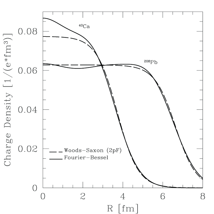
Figure 1: Charge density for ⁴⁰Ca and ²⁰⁸Pb as obtained from elastic electron scattering data.

Additionally, most charge densities determined from electron scattering experiments have been analyzed using model distributions such as the Two-Parameter Fermi or Woods-Saxon distributions. The drawback here is that charge density parameters measured are fundamentally model dependent. This point applies as well to harmonic oscillator or modified harmonic oscillator charge density parameterizations, despite the fact that these have been used to characterize a limited number of nuclei involved in dark matter searches. As noted by Sick Sick1974 , it is at times unclear whether the charge density parameters measured are the fundamental characterization of the nuclear charge density or if they are simply the result of fitting data to a model which may be too restrictive in form. To combat this fundamental uncertainty, model independent methods for analyzing electron scattering data and extracting nuclear charge densities were developed by several groups. Of course, these methods were not completely model independent; some model dependence is necessary since electron scattering data is only available over a finite momentum transfer range. Two primary methods emerged for extracting nuclear charge density parameters in a model independent fashion: an approach in which the charge density is written as a sum of gaussians and an alternate approach in which the charge density is written as a Fourier superposition of Bessel functions.

In the Sum of Gaussians expansion (SOG), first introduced by Sick Sick1974 , the charge density of a nucleus is modelled as a series of Gaussians. The width of the Gaussians, given by the parameter $\gamma$, is calculated by equating it to the smallest width of the peaks in the nuclear wave functions as found in Hartree-Fock calculations; negative amplitudes for the Gaussians are not allowed as to avoid creating structures with widths smaller than $\gamma$ due to interference. As noted in atomic data this method has several advantages: values of $\rho(r)$ at different radii are decoupled due to the rapid fall-off of the Gaussian tail, and as long as a sufficient number of Gaussians are used to ensure a good fit, the results of the analysis is independent of the number of Gaussians.

In the SOG expansion the charge density is written as

$$\rho(r)=\sum_{i=1}^{N}A_{i}\left\{e^{-[(r-R_{i})/\gamma]^{2}}+e^{-[(r+R_{i})/\gamma]^{2}}\right\},$$ (24)

where the coefficients $A_{i}$ are given by

$$A_{i}=\frac{ZeQ_{i}}{2\pi^{3/2}\gamma^{3}\left(1+2R^{2}_{i}/\gamma^{2}\right)}.$$ (25)

The $Q_{i}$ represent the fractional charge carried in the $i^{\rm th}$ gaussian and lead to the following definition for the normalization of the charge density:

$$\sum_{i=1}^{N}Q_{i}=1.$$ (26)

An analytical form factor can be determined for this density parameterization, which eliminates the necessity of performing numerical integration to find the form factor as in the Two-Parameter Fermi density parameterization. Assuming spherical symmetry, the form factor in the SOG expansion is given by

$$F(q)=e^{-q^{2}\gamma^{2}/4}\sum^{N}_{i=1}\frac{Q_{i}}{1+2R^{2}_{i}/\gamma^{2}}\left[\cos(qR_{i})+\frac{2R^{2}_{i}}{\gamma^{2}}\frac{\sin(qR_{i})}{qR_{i}}\right].$$ (27)

The other model independent parameterization of nuclear charge densities that was developed is a Fourier-Bessel expansion. In the Fourier-Bessel expansion (FB), first introduced by Dreher et al. dreher , the charge density is modelled as a sum of Bessel functions up to some cut-off radius $R$, and is assumed to be zero thereafter. The form factor is assumed to fall off for large $q$ as $q^{-4}$ and $e^{-aq^{2}}$; these result from the distribution of nucleons in the nucleus and from the finite extension of the nucleons respectively. Although the results depend slightly on the value of $R$, the cut-off radius, an advantage of this approach is that this collection of assumptions gives an upper limit on the contribution of higher Fourier components to the series expansion atomic data old .

Specifically,

$$\rho(r)=\left\{\begin{array}[]{ll}\sum_{\nu=1}^{N}a_{\nu}j_{0}\left(\nu\pi r/R\right)&\textrm{for}~{}r\leq R,\\ 0&\textrm{for}~{}r\geq R,\end{array}\right.$$ (28)

where $j_{0}(x)=\sin x/x$ is the zero-th order spherical Bessel function. Here the charge density is normalized by requiring

$$\int\rho(r)d^{3}r=Ze.$$ (29)

This charge density also has the advantage that an analytical expression may be found for the form factor. Assuming spherical symmetry, Fourier transforming the charge density yields

$$F(q)=\frac{\sin(qR)}{qR}\,\frac{\displaystyle\sum_{\nu=1}^{N}\frac{\left(-1\right)^{\nu}a_{\nu}}{\nu^{2}\pi^{2}-q^{2}R^{2}}}{\displaystyle\sum_{\nu=1}^{N}\frac{\left(-1\right)^{\nu}a_{\nu}}{\nu^{2}\pi^{2}}},$$ (30)

which is normalized to $F(0)=1$.

In a final point regarding model independent charge densities, it is difficult to estimate the theoretical errors involved in fits to elastic electron scattering data. As noted in atomic data , in the case of the FB approach the errors in the individual coefficients are not presented in data compilations since errors are strongly correlated and can only be extracted from the full correlation matrix; as this matrix is never published in papers, it is impossible to give errors on individual coefficients of the FB expansion for the charge density. Recently, however, Anni, Co’, and Pellegrino in anni analyzed model independent extraction of charge density parameters from elastic electron scattering data to determine uncertainties and the minimum number of expansion coefficients needed to give an accurate representation of the data. Anni et al. determined that in the model independent approach a truncation error is unavoidable; however, they developed an approach to determine an optimal number of coefficients. They point out that distributions extracted from these models must be used with care; however, these models are still much more robust than model dependent fits such as the Woods-Saxon or Two-parameter Fermi model.

IV Nuclear Charge Density Parameters from Muonic Atom Spectroscopy

One can also extract nuclear charge parameter factors from nuclei using muonic atom spectroscopy, however parameters extracted in this manner are to some degree model dependent as the final parameter fitting depends on the choice of an analytical charge density. The nuclear charge distributions are extracted by considering finite size effects to the energy shift in first-order perturbation theory (see muon data old and muon data new , for example, for a review). The analysis takes advantage of Barret moments barret moments which can be extracted in a model independent fashion from the transition energies. Charge density parameters are determined by finding the eigenvalues of the Dirac equation with the analytic charge density fitted to the experimental transition densities muon data new . In the analysis of muonic atom spectroscopy data the Two-Parameter Fermi charge distribution is used:

$$\rho(r)=\frac{\rho_{c}}{e^{(r-c)/a}+1}.$$ (31)

The skin thickness $t=4a\ln(3)$ is fixed to 2.30 fm, and the half-density radius parameter $c$ is fitted to reproduce the experimental transition energies. This method can also be applied to deformed nuclei by writing the half-density radius $c$ as

$$c=R_{0}\left[1+\beta_{2}Y_{20}(\theta,\phi)\right],$$ (32)

where $\beta_{2}$ is the quadrupole deformation parameter, and $R_{0}$ is the monopole radius.

As mentioned previously, the disadvantage to the Two-Parameter Fermi charge density lies in the fact that it has no analytic Fourier transform, and thus form factors must be computed through numerical integration. However, as noted in smith , data from muonic spectroscopy parameterizing the nuclear charge density in terms of a Two-Parameter Fermi distribution exists for several nuclei relevant to direct dark matter detection experiments such as Na, Xe, and I. Two-Parameter Fermi charge distribution parameters also exist for ^184,186W. However, these parameters were obtained from elastic electron scattering experiments. In order to determine the impact of using the Helm versus the form factor associated with the Two-Parameter Fermi charge distribution (and to compare against utilization of the Sum of Gaussian or Fourier-Bessel parameterizations) we numerically fourier transform the Two-Parameter Fermi distribution obtaining the associated form factor, generically referring to it as a Woods-Saxon form factor. Numerical integration was performed with a 48-point Legendre-Gauss quadrature. Although integrating the oscillating $\sin(qr)$ in  6 is notoriously subtle, the 48-point Legendre-Gauss qaudrature used gave robust results and reproduced form factors previously published in the literature (for example, see smith ). The half-density parameter $c$, the parameter $a$ (which is related to the nuclear skin thickness $t$), and the rms value of the charge density for the nuclei of interest are included the the appendix as Table 7.

V Discussion and Results

To determine the effect of using model independent form factors on dark matter direct detection rates, DarkSUSY was modified to compute Helm form factors using the standard parameterizations from eder -engel (referred to here onward as Helm/DarkSUSY-4.1) and the Helm form factors of Lewin and Smith smith (referred to here onward as Helm/Lewin-Smith), as well as model independent form factors derived from the SOG or FB approach. The form factors were evaluated at the appropriate momentum transfers for nuclear recoils between 10 and 100 keV. The 1986 compilation of electron scattering data atomic data was used to calculate the relevant charge densities and form factors. Nuclei were chosen based on their importance to current and future/planned dark matter direct detection searches as well as the availability of electron scattering data in the appropriate momentum transfer range. We have restricted our attention to spin independent scattering of neutralinos from nuclei. This is not too restrictive since many of the nuclei relevant in direct dark matter searches are even-even nuclei for whom the spin dependent cross section vanishes in the $J=0$ ground state (see for example nuclear ). Since the relevant nuclei tend to be spherical or roughly spherical in shape, their charge densities and form factors are able to be analyzed using the SOG or FB approach. Iodine and Sodium (important to the DAMA experiment; see for example DAMA ), Xenon (important to the ZEPLIN and XENON experiments; see for example ZEPLIN and XENON ), and Tungsten (important in the CRESST experiment; see for example CRESST ) are analyzed using the Two-Parameter Fermi charge density as in smith for the sake of completeness.

A range of nuclei from ¹²C to ²⁰⁸Pb were analyzed to give a general trend for increasing nuclear mass. Of particular importance to dark matter experiments are the following nuclei: ²⁸Si (used in the CDMS experiments CDMS ), ³²S (used in the DRIFT experiment DRIFT ), ⁴⁰Ca (used in the CRESST experiments CRESST ), and ^70-74Ge (used in the CDMS, EDELWEISS, GENIUS, and CryoArray experiments CDMS -CryoArray ). For a convenient summary chart of current and future-planned dark matter direct detection experiments and the associated target materials see Tables 1-3 in Gaitskell .

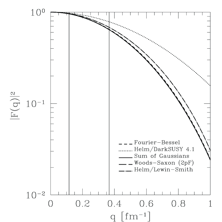
Figure 2: Helm, FB, and SOG form factors for ²⁸Si versus nuclear radius as obtained from elastic electron scattering data. Lines for momentum transfers corresponding to 10 and 100 keV nuclear recoil are included.

In Figure 2 we plot $|F(q)|^{2}$ for ²⁸Si, an important target medium in the CDMS experiments, for small momentum transfers less than 1 fm^-1. Lines indicate the momentum transfers which corresponds to 10 keV and 100 keV nuclear recoils. As can be seen from the plot, all of the form factors in their various parameterizations are not significantly different at low ($\sim$10 keV) nuclear recoils (they differ by at most 2%), and the Helm form factor (in either parameterization) may be used with confidence. However, for larger momentum transfers the FB, SOG, and Woods-Saxon form factors begin to diverge from the Helm form factors; at a momentum transfer corresponding to 100 keV there is a 20.9% difference between the Helm/DarkSUSY-4.1 and the FB/SOG form factors. The Helm form factor of Lewin and Smith differs from the FB or SOG form factors negligibly at small momentum transfers and up to 5% at 100 keV nuclear recoil. Hence for small nuclei at low momentum transfers all parameterizations of the form factor fit well. One should also note, however, that the FB, SOG, and WS form factors, despite the different parameterizations, are virtually indistinguishable, giving further confidence in the use of model independent form factors. The Woods-Saxon form factor is a numerical fourier transform of a physical charge density model (the Two-Parameter Fermi), and should be in some sense thought of as the closest approximation to the actual form factor. The two model independent form factors (FB and SOG) trace the nuclear density more accurately, and easier to use as they are analytic: they should be preferred whenever available.

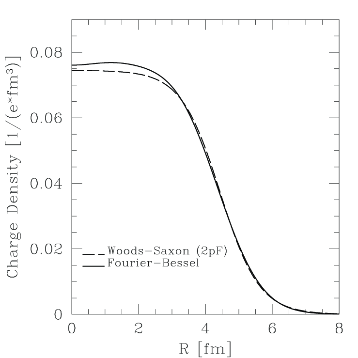
Figure 3: Charge density for ⁷⁰Ge in the Woods-Saxon and FB parameterizations.

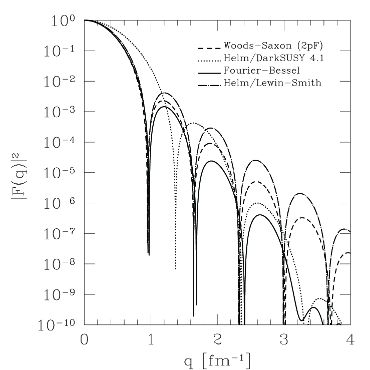
Figure 4: Helm and FB form factors for ⁷⁰Ge.

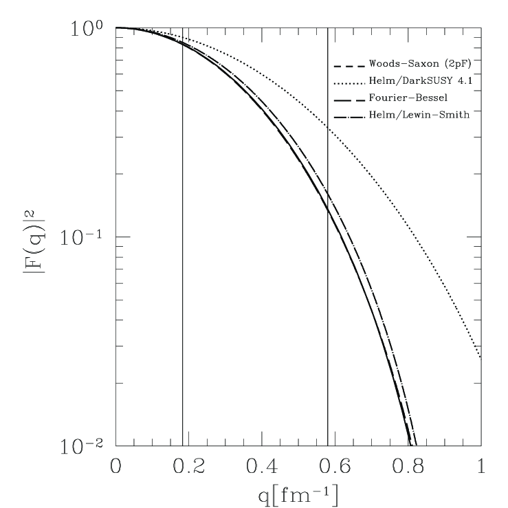
Figure 5: Helm and FB form factors for ⁷⁰Ge with 10 and 100 keV recoil lines for small momentum transfers.

In Figure 3 we plot the charge density for ⁷⁰Ge using both model independent fits to elastic electron scattering data (the FB fit) and also using the standard Woods-Saxon (Two-Parameter Fermi) charge density. As in Figure 1, the charge density for germanium shows a non-constant interior density which cannot be characterized entirely by the Woods-Saxon distribution. Figure 4 shows the Helm/DarkSUSY-4.1, Helm/Lewin-Smith, Woods-Saxon, and FB form factors for ⁷⁰Ge plotted over a range of 0 to 4 fm^-1. As can be seen from the plot, the Helm/DarkSUSY-4.1 and the other form factors differ significantly over the range of momentum transfers. Most significantly, the first diffraction minimum in the FB and WS form factors occurs close to 1 fm^-1 whereas the first minimum in the Helm/DarkSUSY-4.1 form factor occurs at significantly larger momentum transfer. The difference in form factors can be traced to the use of the nuclear radius formula (20), from eder , instead of the more accurate one in Eq. (11), from smith .

Figure 5 shows the same plot of form factors for ⁷⁰Ge but this time highlighting the relevant range of momentum transfers important for direct detection experiments. The momentum transfers corresponding to 10 and 100 keV nuclear recoils are highlighted by vertical lines. Although the divergence between the two form factors at 10 keV nuclear recoil is small (8.12% exactly between Helm/DarkSUSY-4.1 and FB form factors and 2.0% for the Helm/Lewin-Smith and the FB form factors), the form factors are already beginning to diverge. For larger nuclear recoils the form factors continue to diverge leading to a 27.4% and 6.3% difference at 30 keV, a 65.8% and 12.1% difference at 60 keV, and a 148.0% and 19.6% difference at 100 keV for the Helm/DarkSUSY-4.1 vs. the FB and the Helm/Lewin-Smith vs. the FB form factor respectively. Again the WS and FB form factors are indistinguishable over the relevant momentum transfer range. For illustrative purposes, we plot the ratio of the form factor squared in the Helm scheme to that of the form factor squared in the FB expansion for ⁷⁰Ge in Figure 6.

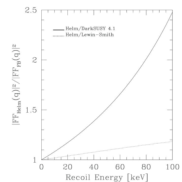
Figure 6: Ratio of the form factors squared in the helm and Fourier Bessel schemes for ⁷⁰Ge.

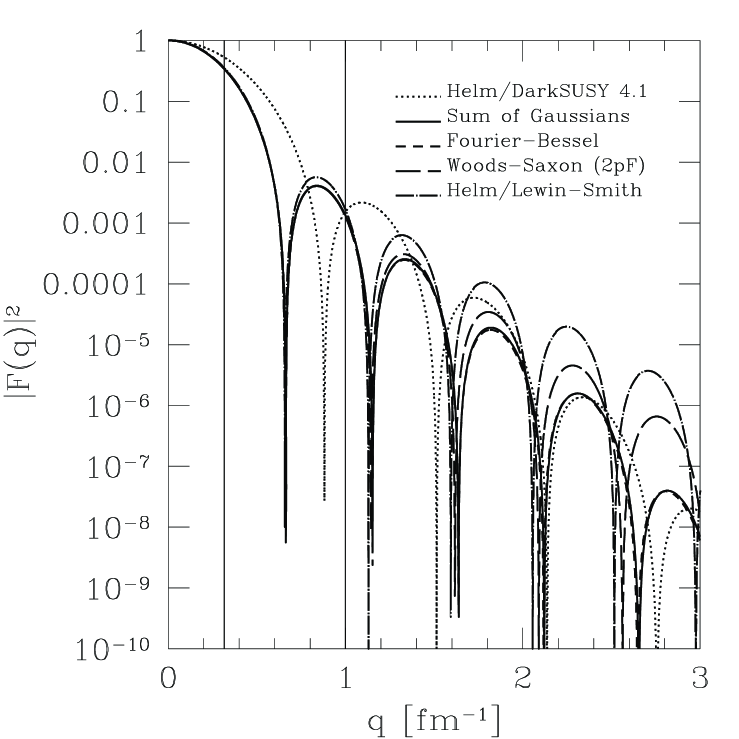
Figure 7: Helm and FB form factors for ²⁰⁸Pb with 10 and 100 keV recoil lines for momentum transfers less than 3.0 fm^-1.

In Figure 7 we plot $|F(q)|^{2}$ for ²⁰⁸Pb for momentum transfers in the range of zero to about 2 fm^-1. Although no direct dark matter searches currently employ lead as a detection medium (though it is used for shielding), lead is an excellent example of the general trend for heavier nuclei. As the atomic number and mass of the nucleus increases, the Helm/DarkSUSY-4.1, FB, SOG, and WS form factors begin to diverge at smaller momentum transfers. As can be seen in the case of ²⁰⁸Pb, the first diffraction minimum for the FB form factor occurs between 0.6 and 0.7 fm^-1 whereas the first diffraction minimum for the Helm/DarkSUSY-4.1 form factor occurs for the much larger momentum transfer of about 0.9 fm^-1. The Helm form factor of Lewin and Smith does a much better job matching the WS, FB, and SOG form factors, however the percent difference can become quite large (as high as 41% as 60 keV recoil energy). This discrepancy leads to a large difference in the spin independent cross sections of neutralinos with ²⁰⁸Pb for nuclear recoils as small as 10 keV. Although these diffraction minima in electron or muon scattering can be partially filled by multiple photon exchanges in the nucleus, in the case of neutralinos this is not expected to occur smith . Lead clearly illustrates the hazards of using large-A nuclei as a detection medium; potential signals may be cut-off due to very small form factors in the relevant range of momentum transfers.

In summary, Table 1 gives the ratios the Helm form factor squared to either FB, SOG, or WS form factors squared for various nuclei important in dark matter searches at 10, 30, 60, and 100 keV nuclear recoils. Note that ²⁷Al is unique in that its Helm form factor as computed in DarkSUSY 4.1 is actually smaller than the corresponding model independent form factor; expected detection rates for an Al target should therefore be higher than previously expected. Table 2 gives the ratio of the Helm/Lewin-Smith form factor squared to either the FB, SOG, or WS form factors squared for various nuclei at a series of nuclear recoil energies.

Nucleus	$F^{2}(q)_{\rm H}/F^{2}(q)$	$F^{2}(q)_{\rm H}/F^{2}(q)$	$F^{2}(q)_{\rm H}/F^{2}(q)$	$F^{2}(q)_{\rm H}/F^{2}(q)$
	10 keV	30 keV	60 keV	100 keV
12C	1.01	1.01	1.03	1.06
16O	1.01	1.03	1.06	1.10
23Na	1.02	1.05	1.10	1.17
27Al	0.99	0.97	0.94	0.90
28Si	1.02	1.06	1.12	1.21
32S	1.02	1.08	1.16	1.28
40Ar	1.03	1.10	1.22	1.41
40Ca	1.03	1.11	1.23	1.42
70Ge	1.08	1.27	1.66	2.48
127I	1.21	1.89	4.98	13739.7⋆
129Xe	1.22	1.92	5.36	1164.1⋆
134Xe	1.22	1.96	5.91	100.8⋆
184W	1.48	4.68	20.80	0.02
208Pb	1.54	6.91	1.64	1.15

Table 1: Ratios of the Helm/DarkSUSY 4.1 DarkSUSY to FB or SOG or WS form factors squared for various nuclei important in current or future direct dark matter searches at 10, 30, 60 and 100 keV nuclear recoil. Lead, though not important in direct dark matter searches, is added as an example of a very large $A$ nucleus.

Nucleus	$F^{2}(q)_{\rm H}/F^{2}(q)$	$F^{2}(q)_{\rm H}/F^{2}(q)$	$F^{2}(q)_{\rm H}/F^{2}(q)$	$F^{2}(q)_{\rm H}/F^{2}(q)$
	10 keV	30 keV	60 keV	100 keV
12C	1.00	1.00	1.01	1.01
16O	1.00	1.01	1.02	1.03
23Na	1.01	1.02	1.03	1.05
27Al	1.00	1.01	1.02	1.04
28Si	1.00	1.01	1.03	1.05
32S	1.01	1.02	1.05	1.08
40Ar	1.01	1.03	1.05	1.09
40Ca	1.01	1.03	1.06	1.1
70Ge	1.02	1.06	1.12	1.19
127I	1.03	1.08	1.13	1.27
129Xe	1.03	1.08	1.13	2.98
134Xe	1.02	1.05	1.03	2.67
184W	1.07	1.25	0.99	1.6
208Pb	1.03	1.01	1.41	1.23

Table 2: Ratios of the Helm/Lewin-Smith form factor smith squared to FB or SOG or WS form factors squared for various nuclei important in current or future direct dark matter searches at 10, 30, 60 and 100 keV nuclear recoil. Lead, though not important in direct dark matter searches, is added as an example of a very large $A$ nucleus.

In Table 1, the starred entries show an extreme difference between the Helm and other form factors in which the ratio is greater than one hundred; this occurs when the form factor is evaluated on or about a diffraction minimum for the WS, FB, or SOG form factors with the corresponding Helm/DarkSUSY-4.1 form factor diffraction minimum occurring at higher momentum transfer. Note that no such entries occur in Table 2 as the Helm/Lewin-Smith form factor has diffraction minima whose placement roughly matches the locations in the FB, SOG, or WS form factors. As can be seen from Tables 1 and 2, although either Helm form factor may be used with confidence for light nuclei ($A<30$) at low nuclear recoils, model independent form factors become increasingly more accurate for large nuclei even at relatively modest momentum transfers. Failure to account for this correction to the form factor can lead to 10–20% errors in cross sections and detection rates.

Figure 8: Hypothetical upper limit on the WIMP-proton cross section for a 100 kg-day exposure of ⁷⁰Ge (assuming an efficiency of 50% and no detected event) and various form factors.

We want to illustrate the importance of using accurate form factors when setting limits on WIMP-proton cross sections. For this purpose, we imagine a hypothetical detector made of ⁷⁰Ge. We assume a simple isothermal sphere model for the WIMPs in the Milky Way halo, so that the WIMP speeds with respect to the halo obey a Maxwellian distribution with a velocity dispersion truncated at the escape velocity. We use the same halo velocity distribution function as sagittarius stream – see particularly (30)-(33) – setting $\sigma_{h}=220$ km/s, $v_{E}=220$ km/s, $v_{\rm esc}=650$ km/s, and $\rho=0.3$ GeV/$c^{2}$/cm³. We assume a detector energy threshold of 10 keV, an efficiency of 50%, an exposure of 100 kg-days, and no events observed in the energy range of 10-50 keV.

In Figure 8 we show the upper limit on the WIMP-proton cross section obtained using (2-5) with $N_{10-50{\rm keV}}<2.3$ and various models of the form factor. The form factor as given by DarkSUSY 4.1 is a Helm type form factor calculated with the parameters given in (19-21). The form factor computed using the procedure in Lewin and Smith smith is a Helm type form factor with parameters given by (11-12). The Fourier Bessel form factor is calculated as in Equation 30 using the data given in Appendix I Table 4. Finally, the form factor labelled “Helm/2pF” is a Helm type form factor computed using $R_{1}$ in (11) with $s=0.9$ fm and with $a=0.5807$ fm and $c=4.430$ fm directly from the Two-Parameter Fermi distribution in table VIII in Fricke et al. (instead of the least-square fit to their table IIIA in Lewin and Smith).

In this example the limits computed with DarkSUSY 4.1 differ from the Fourier Bessel limits by 10–20%, while those computed a la Lewin and Smith differ from the Fourier Bessel limits by 1–2%. (Notice that the logarithmic vertical scale covers a range much smaller than the usual one in this kind of plots.) Numerically, we can compare our hypothetical upper limit on the WIMP-proton cross section for a 100 GeV WIMP, say. Using the Fourier Bessel form factor we find the limit to be $2.38\times 10^{-7}$ pb. Using the Helm form factor with $a$ and $c$ parameters directly from Fricke et al. we find it to be $2.39\times 10^{-7}$ pb, which is 0.5% larger. Using the Helm form factor a la Lewin and Smith we find the limit to be $2.34\times 10^{-7}$ pb, which is 1.5% smaller. Using the Helm form factor computed with DarkSUSY 4.1 we find the upper limit to be $1.93\times 10^{-7}$ pb, which is 19% smaller.

The improvement in form factors that incorporate nuclear data more and more accurately is quite evident in this example. The upper limits on the WIMP-proton cross section calculated using form factors generated with the Helm distribution utilizing muonic spectroscopy data compiled in Fricke et al. muon data new differ only by less than 1% from the WIMP-proton cross section calculated using the Fourier Bessel form factor. The Helm form factor computed a la Lewin and Smith is also a very good approximation to the Fourier Bessel form factor, to within a few percent. The Helm form factor in DarkSUSY 4.1 is further off, by 10–20%, because of a poor choice of the parameter $R_{1}$, which is there set equal to the nuclear radius in standard parameterizations (Eq. 20, from eder ).

VI Charge vs. Mass Form Factors

Neutralinos, of course, interact with the mass distribution of the nucleus, and for neutralino scattering we should be using mass rather than charge form factors. Throughout this paper we have assumed (as have previous authors, for example nuclear ) that the mass and charge distributions within nuclei are roughly proportional. However, there have been recent attempts to pin down the nuclear mass distribution using coherent photoproduction of $\pi^{0}$ mesons pionphotoproduction . Photoproduction of pions is in fact an attractive method for studying nuclear mass distributions; unlike induced hadron reactions it probes the entire nuclear volume. In a recent paper on pion photoproduction massformfactors Krusche analyzed the mass form factors of ¹²C, ⁴⁰Ca and ^natPb using the Helm model for the form factor. He found that rms mass radii were slightly smaller than rms charge radii, though it is still unclear whether these results are real or merely poorly understood systematic effects in the data or in the model dependent calculations. As measurements of coherent photoproduction of pions from nuclei improve, more stringent limits of differences between the nuclear mass and charge densities will be set, including the ability to analyze the data in a model independent fashion as with electron scattering data.

VII Conclusion

In conclusion, significant differences may exist even at relatively low momentum transfers between generic Helm-type and more realistic model independent form factors extracted from elastic electron scattering data, particularly for large $A$ nuclei. These new form factors should be utilized to avoid errors in published limits on neutralino-nucleon cross sections and detection rates in direct dark matter searches. The Fourier Bessel and Sum of Gaussian form factors have the advantage that they are model independent, analytic, and are derived from electron scattering data; we have shown that for calculating upper bounds on the WIMP-proton cross section they are at least as accurate as modified Helm form factors which have been fit for a specific nucleus to muonic spectroscopy data. The FB and SOG form factors have the advantage of existing for the wide array of nuclei being used in current and future planned dark matter detectors, and these parameterizations can be used without the need for extensive fitting to experimental data for different nuclei. We suggest that their use is both simpler and more convenient than modified Helm form factors. Of course, at present, one still must assume that the charge distribution in the nucleus mirrors the mass distribution; however, photo-pion production experiments are beginning to probe nuclear interiors to give model independent parameterizations of the nuclear mass density and should provide a wealth of new data within the next few years.

The model independent analytic form factors in both the Sum of Gaussians (SOG) and Fourier-Bessel (FB) approaches have been incorporated into the DarkSUSY DarkSUSY code along with a numerical integration routine to calculate Fourier transforms of Two-Parameter Fermi distributions; these improvements should appear in the next major public release of the program and will replace the need to rely on the simpler Helm form factor. Parameters in the SOG and FB expansions for the most commonly used target nuclei are included in the appendix.

VIII Acknowledgements

G.D. and A.K. would like to thank Creighton University for a summer research grant which helped support this work. P.G. acknowledges support from the National Science Foundation through grant PHY-0456825.

IX Appendix I: Nuclear Charge Density Parameters for Nuclear Form Factors

Nucleus	12C	16O	28Si	30Si
rms [fm]	2.464(12)	2.737(8)	3.085(17)	3.173(25)
$a_{1}$	0.15721e-1	0.20238e-1	0.33495e-1	0.28397e-1
$a_{2}$	0.38897e-1	0.44793e-1	0.59533e-1	0.54163e-1
$a_{3}$	0.37085e-1	0.33533e-1	0.20979e-1	0.25167e-1
$a_{4}$	0.14795e-1	0.35030e-2	-0.16900e-1	-0.12858e-1
$a_{5}$	-0.44831e-2	-0.12293e-1	-0.14998e-1	-0.17592e-1
$a_{6}$	-0.10057e-1	-0.10329e-1	-0.93248e-3	-0.46722e-2
$a_{7}$	-0.68696e-2	-0.34036e-2	0.33266e-2	0.24804e-2
$a_{8}$	-0.28813e-2	-0.41627e-3	0.59244e-3	0.14760e-2
$a_{9}$	-0.77229e-3	-0.94435e-3	-0.40013e-3	-0.30168e-3
$a_{10}$	0.66908e-4	-0.25771e-3	0.12242e-3	0.483464e-4
$a_{11}$	0.10636e-3	0.23759e-3	-0.12994e-4	0.00000e0
$a_{12}$	-0.36864e-4	-0.10603e-3	-0.92784e-5	-0.51570e-5
$a_{13}$	-0.50135e-5	0.41480e-4	0.72595e-5	0.30261e-5
$a_{14}$	0.94550e-5		-0.42096e-5
$a_{15}$	-0.47687e-5
$R$ [fm]	8.0	8.0	8.0	8.5

Table 3: Fourier-Bessel coefficients for ¹²C, ¹⁶O, ²⁸Si and ³⁰Si as in atomic data , to be used in  (30).

Nucleus	32S	40Ar	40Ca	70Ge
rms [fm]	3.248(4)	3.423(14)	3.450(10)	4.043(2)
$a_{1}$	0.37251e-1	0.30451e-1	0.44846e-1	0.38182e-1
$a_{2}$	0.60248e-1	0.55337e-1	0.61326e-1	0.60306e-1
$a_{3}$	0.14748e-1	0.20203e-1	-0.16818e-2	0.64346e-2
$a_{4}$	-0.18352e-1	-0.16765e-1	-0.26217e-1	-0.29427e-1
$a_{5}$	-0.10347e-1	-0.13578e-1	-0.29725e-2	-0.95888e-2
$a_{6}$	0.30461e-2	-0.43204e-4	0.85534e-2	0.87849e-2
$a_{7}$	0.35277e-2	0.91988e-3	0.35322e-2	0.49187e-2
$a_{8}$	-0.39834e-4	-0.41205e-3	-0.48258e-3	-0.15189e-2
$a_{9}$	-0.97177e-4	0.11971e-3	-0.39346e-3	-0.17385e-2
$a_{10}$	0.92279e-4	-0.19801e-4	0.20338e-3	-0.16794e-3
$a_{11}$	-0.51931e-4	-0.43204e-5	0.25461e-4	-0.11746e-3
$a_{12}$	0.22958e-4	0.61205e-5	-0.17794e-4	0.65768e-4
$a_{13}$	-0.86609e-5	-0.37803e-5	0.67394e-5	-0.30691e-4
$a_{14}$	0.28879e-5	0.18001e-5	-0.21033e-5	0.13051e-5
$a_{15}$	-0.86632e-6	-0.77407e-6		-0.52251e-5
$R$ [fm]	8.0	9.0	8.0	10.0

Table 4: Fourier-Bessel coefficients for ³²S, ⁴⁰Ar, ⁴⁰Ca, and ⁷⁰Ge as in atomic data , to be used in  (30).

Nucleus	72Ge	74Ge	76Ge	208Pb
rms [fm]	4.060(2)	4.075(2)	4.081(2)	5.499(1)
$a_{1}$	0.38083e-1	0.37989e-1	0.37951e-1	0.62732e-1
$a_{2}$	0.59342e-1	0.58298e-1	0.57876e-1	0.38542e-1
$a_{3}$	0.47718e-2	0.27406e-2	0.15303e-2	-0.55105e-1
$a_{4}$	-0.29953e-1	-0.30666e-1	-0.31822e-1	-0.26990e-2
$a_{5}$	-0.88476e-2	-0.81505e-2	-0.76875e-2	0.31016e-1
$a_{6}$	0.96205e-2	0.10231e-1	0.11237e-1	-0.99486e-2
$a_{7}$	0.47901e-2	0.49382e-2	0.50780e-2	-0.93012e-2
$a_{8}$	-0.16869e-2	-0.16270e-2	-0.17293e-2	0.76653e-2
$a_{9}$	-0.15406e-2	-0.13937e-2	-0.15523e-2	0.20886e-2
$a_{10}$	-0.97230e-4	0.15376e-3	0.72439e-4	-0.17840e-2
$a_{11}$	-0.47640e-4	0.14396e-3	0.16560e-3	0.74876e-4
$a_{12}$	-0.15669e-5	-0.73075e-4	-0.86631e-4	0.32278e-3
$a_{13}$	0.67076e-5	0.31998e-4	0.39159e-4	-0.11353e-3
$a_{14}$	-0.44500e-5	-0.12822e-4	-0.16259e-4
$a_{15}$	0.22158e-5	0.48406e-5	0.63681e-5
$R$ [fm]	10.0	10.0	10.0	11.0

Table 5: Fourier-Bessel coefficients for ⁷²Ge, ⁷⁴Ge, ⁷⁶Ge, and ²⁰⁸Pb as in atomic data , to be used in (30).

	12C		16O		28Si
rms [fm]	2.469(6)		2.711		3.121
$i$	$R_{i}$	$Q_{i}$	$R_{i}$	$Q_{i}$	$R_{i}$	$Q_{i}$
1	0.0	0.016690	0.4	0.057056	0.4	0.033149
2	0.4	0.050325	1.1	0.195701	1.0	0.106452
3	1.0	0.138621	1.9	0.311188	1.9	0.206866
4	1.3	0.180515	2.2	0.224321	2.4	0.286391
5	1.7	0.219097	2.7	0.059946	3.2	0.250448
6	2.3	0.278416	3.3	0.135714	3.6	0.056944
7	2.7	0.058779	4.1	0.000024	4.1	0.016829
8	3.5	0.057817	4.6	0.013961	4.6	0.039630
9	4.3	0.007739	5.3	0.000007	5.1	0.000002
10	5.4	0.02001	5.6	0.000002	5.5	0.000938
11	6.7	0.00007	5.9	0.002096	6.0	0.000002
12			6.4	0.000002	6.9	0.002366
RP [fm]	1.20		1.30		1.30

Table 6: Sum of Gaussian coefficients for ¹²C, ¹⁶O, and ²⁸Si as in atomic data , to be used in  (27). RP, the rms radius of the Gaussians, is related to $\gamma$ by RP = $\gamma\sqrt{3/2}$.

	32S		40Ca		208Pb
rms [fm]	3.258		3.480(3)		5.503(2)
$i$	$R_{i}$	$Q_{i}$	$R_{i}$	$Q_{i}$	$R_{i}$	$Q_{i}$
1	0.4	0.045356	0.4	0.042870	0.1	0.003845
2	1.1	0.067478	1.2	0.056020	0.7	0.009724
3	1.7	0.172560	1.8	0.167853	1.6	0.033093
4	2.5	0.324870	2.7	0.317962	2.1	0.000120
5	3.2	0.254889	3.2	0.155450	2.7	0.083107
6	4.0	0.101799	3.6	0.161897	3.5	0.080869
7	4.6	0.022166	4.3	0.053763	4.2	0.139957
8	5.0	0.002081	4.6	0.032612	5.1	0.260892
9	5.5	0.005616	5.4	0.004803	6.0	0.336013
10	6.3	0.000020	6.3	0.004541	6.6	0.033637
11	7.3	0.000020	6.6	0.000015	7.6	0.018729
12	7.7	0.003219	8.1	0.002218	8.7	0.000020
RP [fm]	1.35		1.45		1.70

Table 7: Sum of Gaussian coefficients for ³²S, ⁴⁰Ca, and ²⁰⁸Pb as in atomic data , to be used in  (27). RP, the rms radius of the Gaussians, is related to $\gamma$ by RP = $\gamma\sqrt{3/2}$.

Nucleus	c [fm]	$\left<r^{2}\right>^{1/2}$ [fm]	a [fm]
23Na	2.9393	2.994	0.523
127I	5.5931	4.749	0.523
129Xe	5.6315	4.776	0.523
131Xe	5.6384	4.781	0.523
132Xe	5.6460	4.787	0.523
134Xe	5.6539	4.792	0.523
184W	6.51(7)	5.42(7)	0.535(36)
186W	6.58(3)	5.40(4)	0.480(23)

Table 8: Two-Parameter Fermi coefficients for ²³Na, ¹²⁷I, and ^129-134Xe as in muon data new and for ^184,186W as in atomic data , to be used in  (31). $\left<r^{2}\right>^{1/2}$, the rms value of the charge radius calculated using the Two-Parameter Fermi distribution with $t=2.30$ fm for ²³Na, ¹²⁷I, and ^129-134Xe, and $c$ and $a$ as given above for ^184,186W, is also given.

References

- (1) Bergström L and Gondolo P 1996 Astrop. Phys. 5 263
- (2) Bergström L, Edsjö J and Gondolo P 1997 Phys. Rev. D 55 1765
- (3) Bergström L, Edsjö J and Ullio P 1998 Phys. Rev. D 58 083507
- (4) Bergström L, Edsjö J and Ullio P 1999,Astrophys. J. 526 215
- (5) Baltz E A and Edsjö J 1999 Phys. Rev. D 59 023511
- (6) Edsjö J and Gondolo P 1995 Phys. Lett. B 357 595
- (7) Edsjö J, PhD Thesis (Preprint hep-ph/9704384)
- (8) Bergström L, Damour T, Edsjö J, Krauss L and Ullio P 1999 J. High Energy Phys. JHEP9908 010
- (9) Engel J, Pittel S, and Vogel P 1992 Int. Journal of Mod. Phys. E 1 1-37
- (10) Lewin J D and Smith P F 1996 Astropart. Phys. 6 87-112.
- (11) Gondolo P 1997, in Dark Matter, Quantum Measurements and Experimental Gravitation, XXXI Rencontres de Moriond, Leas Arcs 1996, ed. J. Trân Thanh Vân (Editions Frontière, 1997).
- (12) Gondolo P and Gelmini G 2005 Phys. Rev. D 71 123520
- (13) Uberall P 1971 Electron Scattering from Complex Nuclei (New York: Academic Press)
- (14) Gondolo P, Edsjö J, Ullio P, Bergström L, Schelke M, and Baltz E A 2004 J. Cosmol. Astropart. Phys. 7
- (15) Eder G 1968 Nuclear Forces (MIT Press)
- (16) Jungman G, Kamionkowski M, and Griest K 1996 Phys. Rep. 267 195
- (17) Engel J 1991 Phys. Lett. B 264 114
- (18) Helm R 1956 Phys. Rev. 104 1466
- (19) Hofstadter R et al. 1977 Phys. Rev. Lett. 38 152
- (20) De Vries H et al. 1987 Atomic Data and Nuclear Data 36 495-529
- (21) De Jager et al. 1974 Atomic Data and Nuclear Data Tables 14 479
- (22) Engfer R et al. 1974 Atomic Data and Nuclear Data Tables 14 509-597
- (23) Fricke G et al. 1995 Atomic Data and Nuclear Data Tables 60 177-285
- (24) Barrett R 1970 Phys. Rev. Lett. B 33 388
- (25) Frauenfelder H and Henley E 1991 Subatomic Physics 2nd Ed. (New York: Prentice Hall)
- (26) Sick I 1974 Nucl. Phys. A 218 509-541
- (27) Dreher et al. 1974 Nucl. Phys. A 235 219-248.
- (28) Anni R, Co’ G and Pellegrino P 1995 Nucl.Phys. A 584 35-59
- (29) Bernabei R et al. [DAMA col.] 2000 Phys. Lett. B 480 23
- (30) Alner G J et al. [UK Dark Matter Collaboration] 2005 Astropart. Phys. 23 444-462
- (31) Aprile E et al. 2005 New Astron. Rev. 49 289-295
- (32) Akerib D S et al. 2006 Phys. Rev. Lett. 96 011302
- (33) Luca M [EDELWEISS Collaboration] (Preprint astro-ph/0605496)
- (34) Alner G J et al. 2005 Nucl. Instrum. Meth. A 555 173
- (35) Angloher G et. al. 2005, Astropar. Phys. 23 325-339
- (36) Schnee R, Akerib D, and Gaitskell R 2003 Nucl. Phys. Proc. Suppl. 124 233-236
- (37) Gaitskell R 2004 Annu. Rev. Nucl. Part. Sci. 54 315-359
- (38) Freese K, Gondolo P, and Newberg H 2005 Phys. Rev. D 71 043516
- (39) Akerib DS et al. 2004 Phys Rev Lett. 93 211301
- (40) Krusche B et al. 2002 Phys. Rev. Lett. B 526 287
- (41) Krusche B 2005 Eur. Phys. J. A 26 7-18