Modeling dihadron fragmentation functions

Abstract

We present a model for dihadron fragmentation functions, describing the fragmentation of a quark into two unpolarized hadrons. We tune the parameters of our model to the output of the PYTHIA event generator for two-hadron semi-inclusive production in deep inelastic scattering at HERMES. Once the parameters of the model are fixed, we make predictions for other unknown fragmentation functions and for a single-spin asymmetry in the azimuthal distribution of $\pi^{+}\pi^{-}$ pairs in semi-inclusive deep inelastic scattering on a transversely polarized target at HERMES and COMPASS. Such asymmetry could be used to measure the quark transversity distribution function.

I Introduction

Dihadron Fragmentation Functions (DiFF) describe the probability that a quark hadronizes into two hadrons plus anything else, i.e. the process $q\to H_{1}\,H_{2}\,X$. They can appear in any process where hadronization is involved, in particular in lepton-lepton, lepton-hadron and hadron-hadron collisions producing final-state hadrons. They carry information that is not accessible to single-hadron fragmentation functions, but on the other hand they are more complex to study and to measure.

Unpolarized DiFF were introduced for the first time by Konishi, Ukawa and Veneziano Konishi et al. (1978). Their evolution equations have been studied in Refs. Vendramin (1981); Sukhatme and Lassila (1980) and more recently reanalyzed in Refs. de Florian and Vanni (2004); Majumder and Wang (2004, 2005). All these studies focused on the probability of producing two hadrons with energy fractions $z_{1}$ and $z_{2}$ by integrating over the invariant mass of the produced pair. However, it is fair to say that the only experimental information related to unpolarized DiFF consists of invariant mass spectra of hadron pairs produced in $e^{+}e^{-}$ annihilation Acton et al. (1992); Abreu et al. (1993); Buskulic et al. (1996), Semi-Inclusive Deep-Inelastic Scattering (SIDIS) Cohen et al. (1982); Aubert et al. (1983); Arneodo et al. (1986) and proton-proton collisions Blobel et al. (1974); Aguilar-Benitez et al. (1991); Adams et al. (2004). Recently, it has been suggested to use DiFF as tools to investigate the in-medium effects in heavy-ion collisions Adams et al. (2004); Fachini (2004); Majumder and Wang (2004, 2005); Majumder (2005). To address this and other issues, it is necessary to improve our knowledge of unpolarized DiFF in vacuum.

DiFF can be used also for spin studies. In particular, they can act as analyzers of the spin of the fragmenting quark Efremov et al. (1992); Collins et al. (1994); Collins and Ladinsky (1994); Jaffe et al. (1998); Artru and Collins (1996) and they can be used to study vector meson polarization Efremov and Teryaev (1982); Ji (1994); Anselmino et al. (1999); Bacchetta and Mulders (2000). The definition and properties of all possible DiFF for two unpolarized detected hadrons have been presented in Ref. Bianconi et al. (2000a) up to leading twist, and in Ref. Bacchetta and Radici (2004a) up to subleading twist integrated over the transverse component of the center-of-mass (cm) momentum of the hadron pair. Despite the wealth of observables related to polarized DiFF, experimental information is limited Abreu et al. (1997); Abbiendi et al. (2000); Abe et al. (1995).

At present, the most important application of polarized DiFF appears to be the measurement of the quark transversity distribution in the nucleon. This function, $h_{1}$, represents the probabilistic distribution of transversely polarized partons inside transversely polarized hadrons, and is a missing cornerstone to complete the knowledge of the leading-order (spin) structure of the nucleon (for a review see Ref. Barone and Ratcliffe (2003)). Being a chiral-odd function, $h_{1}$ needs to be combined with another chiral-odd soft function. The simplest possibility is to consider double-spin asymmetries in polarized Drell-Yan processes Ralston and Soper (1979). This option is under investigation at BNL using high-energy polarized proton-proton collisions Soffer et al. (2002); Bianconi and Radici (2006) and could be studied also at GSI using polarized proton-antiproton collisions Anselmino et al. (2003); Efremov et al. (2004); Bianconi and Radici (2005a, b).

Another possibility is to measure Single-Spin Asymmetries (SSA) in the SIDIS production of a pion on transversely polarized targets. Recent data have been released using proton Airapetian et al. (2005); Diefenthaler (2005) and deuteron Alexakhin et al. (2005) targets. Their interpretation advocates the so-called Collins effect Collins (1993), by which a leading-twist contribution to the cross section appears where $h_{1}$ is convolved with the Collins function $H_{1}^{\perp}$, a fragmentation functions that describes the decay probability of a transversely polarized quark into a single pion. However, extracting $h_{1}$ from SSA data requires the cross section to depend explicitly upon the transverse momentum of the detected pion with respect to the photon axis Boer and Mulders (1998). This fact brings in several complications, including the possible overlap of the Collins effect with other competing mechanisms and more complicated factorization proofs and evolution equations Collins and Metz (2004); Ji et al. (2005).

Semi-inclusive production of two hadrons Collins et al. (1994); Jaffe et al. (1998) offers an alternative way to access transversity, where the chiral-odd partner of transversity is represented by the DiFF $H_{1}^{{<\kern-2.10002pt{\scriptscriptstyle)}}}$ Radici et al. (2002), which relates the transverse spin of the quark to the azimuthal orientation of the two-hadron plane. This function is at present unknown. Very recently, the HERMES collaboration has reported measurements of the asymmetry containing the product $h_{1}H_{1}^{{<\kern-2.10002pt{\scriptscriptstyle)}}}$ van der Nat (2005). The COMPASS collaboration has also presented analogous preliminary results Martin (2006). In the meanwhile, the BELLE collaboration is planning to measure the fragmentation functions $H_{1}^{{<\kern-2.10002pt{\scriptscriptstyle)}}}$ in the near future Hasuko et al. (2003); Abe et al. (2006).

In this context, it seems of great importance to devise a way to model DiFF. From the theoretical side, this can help understanding what are the essential building blocks and mechanisms involved in dihadron fragmentation. It can also provide a guidance for fits to data and further phenomenological studies. From the experimental side, a model could be useful to study the effects of cuts and acceptance, to estimate the size of observables in different processes and kinematical regimes. Our work is not the first one in this direction Jaffe et al. (1998); Bianconi et al. (2000b); Radici et al. (2002). The model presented here is close to the one discussed in Ref. Radici et al. (2002). However, for the first time we are able to fix the parameters by comparing our unpolarized DiFF $D_{1}$ with the output of the PYTHIA event generator Sjostrand et al. (2001) tuned for HERMES Liebing (2004). Then, without introducing extra parameters, we make predictions for the polarized DiFF $H_{1}^{{<\kern-2.10002pt{\scriptscriptstyle)}}}$ and the related SSA involving the transversity distribution $h_{1}$.

The paper is organized as follows. In Sec. II, we review the basic formalism of DiFF and of SIDIS cross section for two-hadron production. In Sec. III, we describe our model for the fragmentation of a quark into two unpolarized hadrons and give analytic results for DiFF calculated in this model. In Sec. IV, we fix the parameters of the model by comparing it to the output of the PYTHIA event generator tuned for HERMES kinematics. In Sec. V, we show numerical predictions for the DiFF and for the above-mentioned SSA in the kinematics explored by the HERMES van der Nat (2005) and COMPASS collaborations Martin (2006). Finally, in Sec. VI we draw some conclusions.

II Basics of dihadron fragmentation functions

Dihadron Fragmentation Functions are involved in the description of the fragmentation process $q\to\pi^{+}\pi^{-}X$. The quark has momentum $k$. The two pions have masses $m_{\pi}=0.140$ GeV, momenta $P_{1}$ and $P_{2}$, respectively, and invariant mass $M_{h}$ (considered to be much smaller than the hard scale of the process, e.g., the virtuality of the photon, $Q$, in SIDIS). We introduce the vectors $P_{h}=P_{1}+P_{2}$ and $R=(P_{1}-P_{2})/2$. We describe a 4-vector $a$ as $[a^{-},a^{+},a^{x},a^{y}]$, i.e. in terms of its light-cone components $a^{\pm}=(a^{0}\pm a^{3})/\sqrt{2}$ and its transverse spatial components. We introduce the light-cone fraction $z=P_{h}^{-}/k^{-}$ and the polar angle $\theta$, being the angle between the direction of $P_{1}$ in the pair’s center of mass and the direction of $P_{h}$ in the lab frame Bacchetta and Radici (2003), so that the relevant momenta can be written as

$$k^{\mu} =\biggl{[}\frac{P_{h}^{-}}{z},\;\frac{z(k^{2}+\vec{k}_{T}^{2})}{2P_{h}^{-}},\;k_{T}^{x},k_{T}^{y}\biggr{]},$$ (1)

$$P_{h}^{\mu} =\biggl{[}P_{h}^{-},\;\frac{M_{h}^{2}}{2P_{h}^{-}},\;0,\;0\biggr{]},$$ (2)

$$R^{\mu} =\biggl{[}\frac{|\vec{R}|\,P_{h}^{-}}{M_{h}}\,\cos{\theta},\;-\frac{|\vec{R}|\,M_{h}}{2\,P_{h}^{-}}\,\cos{\theta},\;R_{T}^{x},R_{T}^{y}\biggr{]}$$

$$=\biggl{[}\frac{|\vec{R}|\,P_{h}^{-}}{M_{h}}\,\cos{\theta},\;-\frac{|\vec{R}|\,M_{h}}{2\,P_{h}^{-}}\,\cos{\theta},\ |\vec{R}|\,\sin{\theta}\,\cos{\phi_{R}},\;|\vec{R}|\,\sin{\theta}\,\sin{\phi_{R}}\biggr{]},$$ (3)

where

$$|\vec{R}|=\frac{M_{h}}{2}\sqrt{1-\frac{4\,m_{\pi}^{2}}{M_{h}^{2}}},$$ (4)

and $\phi_{R}$ is defined later in Eq. (15) (see also Fig. 1). It is useful to compute the scalar products

$$P_{h}\cdot R =0,$$ (5)

$$P_{h}\cdot k =\frac{M_{h}^{2}}{2z}+z\,\frac{k^{2}+|\vec{k}_{T}|^{2}}{2},$$ (6)

$$R\cdot k =\biggl{(}\frac{M_{h}}{2\,z}-z\,\frac{k^{2}+|\vec{k}_{T}|^{2}}{2\,M_{h}}\biggr{)}\,|\vec{R}|\,\cos{\theta}-\vec{k}_{T}\cdot\vec{R}_{T}.$$ (7)

Fragmentation functions are extracted from the correlation function Bacchetta and Radici (2003)

$$\Delta^{q}(z,\cos\theta,M_{h}^{2},\phi_{R})=\frac{z|\vec{R}|}{16\,M_{h}}\int d^{2}\vec{k}_{T}\;dk^{+}\,\Delta^{q}(k;P_{h},R)\Big{|}_{k^{-}=P_{h}^{-}/z}\;,$$ (8)

where Boer et al. (2003); Bacchetta and Radici (2004a)

$$\begin{split}\Delta^{q}(k,P_{h},R)_{ij}&=\sum_{X}\,\int\frac{d^{4}\xi}{(2\pi)^{4}}\;e^{+{\rm i}k\cdot\xi}\langle 0|{\cal U}^{n_{+}}_{(-\infty,\xi)}\,\psi_{i}^{q}(\xi)|P_{h},R;X\rangle\langle P_{h},R;,X|\bar{\psi}_{j}^{q}(0)\,{\cal U}^{n_{+}}_{(0,-\infty)}|0\rangle\,.\end{split}$$ (9)

Since we are going to perform the integration over the transverse momentum $\vec{k}_{T}$, the Wilson lines ${\cal U}$ can be reduced to unity using a light-cone gauge.

The only fragmentation functions surviving after $\vec{k}_{T}$-integration are Bianconi et al. (2000a); Bacchetta and Radici (2003)

$$D_{1}^{q}(z,\cos\theta,M_{h}^{2}) =4\pi\,\text{Tr}[\Delta^{q}(z,\cos\theta,M_{h}^{2},\phi_{R})\,\gamma^{-}],$$ (10)

$$\frac{\epsilon_{T}^{ij}\,R_{Tj}}{M_{h}}\,H_{1}^{{<\kern-2.10002pt{\scriptscriptstyle)}}\,q}(z,\cos\theta,M_{h}^{2}) =4\pi\,\text{Tr}[\Delta^{q}(z,\cos\theta,M_{h}^{2},\phi_{R})\,i\,\sigma^{i-}\,\gamma_{5}].$$ (11)

These functions can be expanded in the relative partial waves of the pion pair system. Truncating the expansion at the $p$-wave level we obtain Bacchetta and Radici (2003)

$$D_{1}^{q}(z,\cos{\theta},M_{h}^{2}) \approx D_{1,oo}^{q}(z,M_{h}^{2})+D_{1,ol}^{q}(z,M_{h}^{2})\,\cos\theta+D_{1,ll}^{q}(z,M_{h}^{2})\,\frac{1}{4}\,(3\cos^{2}\theta-1)\;,$$ (12)

$$H_{1}^{{<\kern-2.10002pt{\scriptscriptstyle)}}\,q}(z,\cos{\theta},M_{h}^{2}) \approx H_{1,ot}^{{<\kern-2.10002pt{\scriptscriptstyle)}}\,q}(z,M_{h}^{2})+H_{1,lt}^{{<\kern-2.10002pt{\scriptscriptstyle)}}\,q}(z,M_{h}^{2})\,\cos\theta\;.$$ (13)

The fragmentation function $D_{1,oo}$ can receive contributions from both $s$ and $p$ waves, but not from the interference between the two, $D_{1,ol}$ and $H_{1,ot}^{{<\kern-2.10002pt{\scriptscriptstyle)}}}$ originate from the interference of $s$ and $p$ waves, $D_{1,ll}$ comes from polarized $p$ waves, and $H_{1,lt}^{{<\kern-2.10002pt{\scriptscriptstyle)}}}$ originates from the interference of two $p$ waves with different polarization.

Our model can make predictions for the above fragmentation functions as well as for transverse-momentum-dependent fragmentation functions, which we do not consider in this Section. However, we will focus our attention mainly on the functions $D_{1,oo}$ and $H_{1,ot}^{{<\kern-2.10002pt{\scriptscriptstyle)}}}$ because of their relevance for transversity measurements in SIDIS Collins et al. (1994); Jaffe et al. (1998); Radici et al. (2002); Bacchetta and Radici (2004b).

Let’s consider in fact the SIDIS process $l\,p\to l^{\prime}\,\pi^{+}\,\pi^{-}\,X$, where $l$ and $l^{\prime}$ are the momenta of the lepton before and after the scattering and $q=l-l^{\prime}$ is the momentum of the virtual photon. We consider the cross section differential in $dM_{h}^{2}$, $d\phi_{R}$, $dz$, $dx$, $dy$, $d\phi_{S}$, where $z$, $x$, $y$ are the usual scaling variables employed in SIDIS, and the azimuthal angles are defined so that (see Fig. 1)

$$\cos\phi_{S} =\frac{(\hat{q}\times\vec{l})}{|\hat{q}\times\vec{l}|}\cdot\frac{(\hat{q}\times\vec{S})}{|\hat{q}\times\vec{S}|}, \sin\phi_{S} =\frac{(\vec{l}\times\vec{S})\cdot\hat{q}}{|\hat{q}\times\vec{l}|\,|\hat{q}\times\vec{S}|},$$ (14)

$$\cos\phi_{R} =\frac{(\hat{q}\times\vec{l})}{|\hat{q}\times\vec{l}|}\cdot\frac{(\hat{q}\times\vec{R_{T}})}{|\hat{q}\times\vec{R_{T}}|}, \sin\phi_{R} =\frac{(\vec{l}\times\vec{R_{T}})\cdot\hat{q}}{|\hat{q}\times\vec{l}|\,|\hat{q}\times\vec{R_{T}}|},$$ (15)

where $\hat{q}=\vec{q}/|\vec{q}|$ and $\vec{R_{T}}$ is the component of $R$ perpendicular to $P_{h}$.

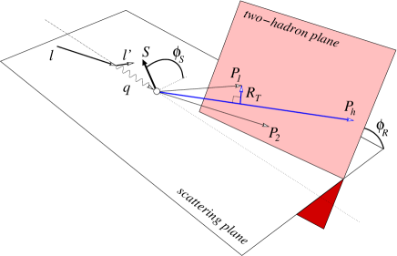
Figure 1: Angles involved in the measurement of the transverse single-spin asymmetry in deep-inelastic production of two hadrons in the current region.

When the target is transversely polarized, we can define the following cross section combinations 

$$d^{6}\!\sigma_{UU} =\frac{d^{6}\!\sigma^{\uparrow}+d^{6}\!\sigma^{\downarrow}}{2}=\sum_{q}\frac{\alpha^{2}e_{q}^{2}}{\pi\,y\,Q^{2}}\,\frac{1-y+y^{2}/2+y^{2}\,\gamma^{2}/4}{1+\gamma^{2}}\,f_{1}^{q}(x)\,D_{1,oo}^{q}(z,M_{h}^{2}),$$ (16)

$$d^{6}\!\sigma_{UT} =\frac{d^{6}\!\sigma^{\uparrow}-d^{6}\!\sigma^{\downarrow}}{2}=-\sum_{q}\frac{\alpha^{2}e_{q}^{2}}{4\,y\,Q^{2}}\,\frac{1-y-y^{2}\,\gamma^{2}/4}{1+\gamma^{2}}\,\sin(\phi_{R}+\phi_{S})\,h_{1}^{q}(x)\,\frac{|\vec{R}|}{M_{h}}\,H_{1,ot}^{{<\kern-2.10002pt{\scriptscriptstyle)}}q}(z,M_{h}^{2}),$$ (17)

where $\alpha$ is the fine structure constant, $\gamma=2Mx/Q$, and $M$ is the mass of the target. These expressions are valid up to leading twist only. Subleading contributions are described in Ref. Bacchetta and Radici (2004a). In particular, they give rise to a term proportional to $\cos\phi_{R}$ in $d\sigma_{UU}$ and a term proportional to $\sin\phi_{S}$ in $d\sigma_{UT}$. Corrections at order $\alpha_{S}$ were partially studied in Ref. de Florian and Vanni (2004), but further work is required.

We can define the asymmetry amplitude

$$A_{UT}^{\sin(\phi_{R}+\phi_{S})}(x,y,z,M_{h}^{2})\equiv\frac{1}{\sin(\phi_{R}+\phi_{S})}\,\frac{d^{6}\!\sigma_{UT}}{d^{6}\!\sigma_{UU}}=-\frac{\frac{1-y-y^{2}\,\gamma^{2}/4}{x\,y^{2}\,(1+\gamma^{2})}}{\frac{1-y+y^{2}/2+y^{2}\,\gamma^{2}/4}{x\,y^{2}\,(1+\gamma^{2})}}\,\frac{\pi\,|\vec{R}|}{4\,M_{h}}\frac{\sum_{q}e_{q}^{2}\,h_{1}^{q}(x)\ H_{1,ot}^{{<\kern-2.10002pt{\scriptscriptstyle)}}q}(z,M_{h}^{2})}{\sum_{q}e_{q}^{2}\,f_{1}^{q}(x)\ D_{1,oo}^{q}(z,M_{h}^{2})}.$$ (18)

Note that we avoided simplifying the prefactors because numerator and denominator are usually integrated separately over some of the variables.

III Fragmentation functions in a spectator model

We aim at describing the process $q\to\pi^{+}\pi^{-}X$ at invariant mass $M_{h}\lesssim 1.3$ GeV. To have an idea of the prominent channels contributing to this process, we examined the output of the PYTHIA event generator Sjostrand et al. (2001) tuned for HERMES Liebing (2004), which well reproduces the measured events at HERMES. Further details concerning the event generator’s output will be discussed in the next section. Fig. 2 shows the number of counted dihadron pairs in bins of $M_{h}$ (200 bins from 0.3 to 1.3 GeV). The total amount of events is 2667889.

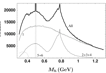
Figure 2: Semi-inclusive dihadron counts in bins of $M_{h}$ from the PYTHIA event generator Sjostrand et al. (2001) tuned for HERMES Liebing (2004). The thick solid line represents the sum of all channels. The thin solid line represents the sum of channels 2,3, and 4 described in the text. The dashed line represents the sum of channels 5 and 6 (which are excluded in our model). The gray line is the difference between the total and the sum of all channels 2 to 6 and is assumed to represent channel 1.

A few prominent channels contribute to this process:

1. $q\to\pi^{+}\pi^{-}X_{1}$: fragmentation into an “incoherent” $\pi^{+}\pi^{-}$ pair that we will call, in the following, “background”;

2. $q\to\rho\ X_{2}\to\pi^{+}\pi^{-}X_{2}$: fragmentation into a $\rho$ resonance decaying into $\pi^{+}\pi^{-}$, responsible for a peak at $M_{h}\sim$ 770 MeV (14.81%);

3. $q\to\omega\ X_{3}\to\pi^{+}\pi^{-}X_{3}$: fragmentation into a $\omega$ resonance decaying into $\pi^{+}\pi^{-}$, responsible for a small peak at $M_{h}\sim$ 782 MeV (0.31%);

4. $q\to\omega\ X_{4}^{\prime}\to\pi^{+}\pi^{-}X_{4}$ with $X_{4}=\pi^{0}\ X_{4}^{\prime}$: fragmentation into a $\omega$ resonance decaying into $\pi^{+}\pi^{-}\pi^{0}$ ($\pi^{0}$ unobserved), responsible for a broad peak around $M_{h}\sim$ 500 MeV (8.65%);

5. $q\to\eta\ X_{5}^{\prime}\to\pi^{+}\pi^{-}X_{5}$ with $X_{5}={\cal X}\ X_{5}^{\prime}$: fragmentation into a $\eta(547)$ or $\eta^{\prime}(958)$ decaying into $\pi^{+}\pi^{-}{\cal X}$ (${\cal X}$ unobserved), responsible for a peak around $M_{h}\sim$ 350 MeV (2.05%);

6. $q\to K^{0}\ X_{6}\to\pi^{+}\pi^{-}X_{6}$: fragmentation into a $K^{0}$ resonance decaying into $\pi^{+}\pi^{-}$, responsible for a narrow peak at $M_{h}\sim$ 498 MeV (3.41%).

On top of these, there could be the presence of two other channels:

1. $q\to\sigma\ X_{7}\to\pi^{+}\pi^{-}X_{7}$: fragmentation into the largely debated $\sigma$ resonance (see, e.g., Ref. Caprini et al. (2006)) decaying into $\pi^{+}\pi^{-}$, which could be responsible for a very broad peak anywhere between 400 and 1200 MeV;

2. $q\to f_{0}\ X_{8}\to\pi^{+}\pi^{-}X_{8}$: fragmentation into a $f_{0}$ resonance decaying into $\pi^{+}\pi^{-}$, which should give rise to a peak at $M_{h}\sim$ 980 MeV, not evident in the output of PYTHIA.

In our model, we considered only channels 1 to 6. All events not belonging to channels 2 to 6 were included in channel 1, which then contains 70.77% of the total events.

We work in the framework of a “spectator” model for the fragmentation process: for $q\to\pi^{+}\pi^{-}X$, the sum over all possible intermediate states $X$ is replaced by an effective on-shell state – the spectator – whose quantum numbers are in this case the same as the initial quark and whose mass is one of the parameters of the model. In principle, different channels could produce spectators with different masses. Moreover, each channel could end up into more than one possible spectator Kitagawa and Sakemi (2000). For sake of simplicity, here we consider just a single spectator for all channels. We shall denote its mass as $M_{s}$ and its momentum as $P_{s}$. The choice of using the same spectator for all channels implies in particular that the fragmentation amplitudes of all channels can interfere with each other maximally. In reality, it is plausible that only a fraction of the total events ends up in the same spectator and can thus produce interference effects.

Pions in channels 2 and 3 are obviously produced in relative $p$ wave, since they come from the decay of a vector meson. In channel 4, each charged pion can be in a relative $p$ wave with respect to the other one or to $\pi^{0}$, the net result being that there is a fraction of $\pi^{+}\pi^{-}$ pairs that is produced in a relative $s$ wave. In the following, we will neglect this fraction and assume that all charged pairs are produced in $p$ wave; at present we don’t have enough information to discriminate the two contributions. This assumption is most probably inadequate and would lead to an overestimate of the contribution of channel 4 to the final single spin asymmetry.

We further assume that all pions in channel 1 are produced in $s$ wave. It is possible that a fraction of the background events are also produced in $p$ wave. However, such a fraction cannot be too big, as it would give rise to interference effects that would distort the shape of the $\rho$ meson peak. It is actually known that such a distortion can indeed occur, but also that it is not big Lafferty (1993); Buskulic et al. (1996). We think that this point deserves further attention, but should not change the main features of our results.

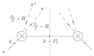
Figure 3: Diagrammatic representation of the correlation function $\Delta$ in the spectator model.

We model the correlation function in the following way (see Fig. 3):

$$\begin{split}\Delta^{q}(k,P_{h},R)&=\frac{1}{(2\pi)^{4}}\,\frac{(\kern 1.99997ptk\kern-4.49997pt/+m)}{k^{2}-m^{2}}\,\Bigl{(}F^{s\star}\,e^{-\frac{k^{2}}{\Lambda_{s}^{2}}}+F^{p\star}\,e^{-\frac{k^{2}}{\Lambda_{p}^{2}}}\,\kern 1.99997ptR\kern-5.0pt/\Bigr{)}\,(\kern 1.99997ptk\kern-4.49997pt/-\kern 1.99997ptP\kern-5.0pt/_{h}+M_{s})\,\\ &\quad\times\Bigl{(}F^{s}\,e^{-\frac{k^{2}}{\Lambda_{s}^{2}}}+F^{p}\,e^{-\frac{k^{2}}{\Lambda_{p}^{2}}}\,\kern 1.99997ptR\kern-5.0pt/\Bigr{)}\,\frac{(\kern 1.99997ptk\kern-4.49997pt/+m)}{k^{2}-m^{2}}\,2\pi\,\delta\bigl{(}(k-P_{h})^{2}-M_{s}^{2}\bigr{)}\,.\end{split}$$ (19)

Isospin symmetry implies that the fragmentation correlator for $u\to\pi^{+}\pi^{-}X$ is the same as for $\bar{d}\to\pi^{+}\pi^{-}X$, $d\to\pi^{-}\pi^{+}X$, $\bar{u}\to\pi^{-}\pi^{+}X$. Therefore, the result for $d$ and $\bar{u}$ quarks can be obtained from the result for $u$ quark by simply changing the sign of $\vec{R}$, i.e. changing $\theta\to\pi-\theta$ and $\phi\to\phi+\pi$. From now on we will drop the superscript indicating the quark flavor and calculate the fragmentation functions for $u\to\pi^{+}\pi^{-}X$. The terms with vertex $F^{s}$ refer to the $s$-wave contribution, the terms with vertex $F^{p}$ to the $p$-wave contribution. The exponential form factors suppress the contributions from high quark virtualities Gamberg et al. (2003). Other possibilities can be considered, e.g., dipole form factors Bianconi et al. (2000b); Radici et al. (2002), or sharp cutoffs Bacchetta et al. (2002).

Inserting Eq. (19) into Eq. (8), we get

$$\begin{split}\Delta(z,\cos\theta,M_{h}^{2},\phi_{R})&=\frac{|\vec{R}|}{128\,\pi^{2}\,M_{h}}\,\frac{z^{2}}{2\,(1-z)\,P_{h}^{-}}\int d|\vec{k}_{T}|^{2}\,\biggl{[}|F^{s}|^{2}\,e^{-\frac{2\,k^{2}}{\Lambda_{s}^{2}}}\,\frac{(\kern 1.99997ptk\kern-4.49997pt/+m)\,(\kern 1.99997ptk\kern-4.49997pt/-\kern 1.99997ptP\kern-5.0pt/_{h}+M_{s})\,(\kern 1.99997ptk\kern-4.49997pt/+m)}{(k^{2}-m^{2})^{2}}\\ &\quad+|F^{p}|^{2}\,e^{-\frac{2\,k^{2}}{\Lambda_{p}^{2}}}\,\frac{(\kern 1.99997ptk\kern-4.49997pt/+m)\,\kern 1.99997ptR\kern-5.0pt/\;(\kern 1.99997ptk\kern-4.49997pt/-\kern 1.99997ptP\kern-5.0pt/_{h}+M_{s})\,\kern 1.99997ptR\kern-5.0pt/\;\,(\kern 1.99997ptk\kern-4.49997pt/+m)}{(k^{2}-m^{2})^{2}}\\ &\quad+F^{s\star}\,F^{p}\,e^{-k^{2}\,\frac{\Lambda_{s}^{2}+\Lambda_{p}^{2}}{\Lambda_{s}^{2}\,\Lambda_{p}^{2}}}\,\frac{(\kern 1.99997ptk\kern-4.49997pt/+m)\,(\kern 1.99997ptk\kern-4.49997pt/-\kern 1.99997ptP\kern-5.0pt/_{h}+M_{s})\,\kern 1.99997ptR\kern-5.0pt/\;\,(\kern 1.99997ptk\kern-4.49997pt/+m)}{(k^{2}-m^{2})^{2}}\\ &\quad+F^{s}\,F^{p\star}\,e^{-k^{2}\,\frac{\Lambda_{s}^{2}+\Lambda_{p}^{2}}{\Lambda_{s}^{2}\,\Lambda_{p}^{2}}}\,\frac{(\kern 1.99997ptk\kern-4.49997pt/+m)\,\kern 1.99997ptR\kern-5.0pt/\;(\kern 1.99997ptk\kern-4.49997pt/-\kern 1.99997ptP\kern-5.0pt/_{h}+M_{s})\,(\kern 1.99997ptk\kern-4.49997pt/+m)}{(k^{2}-m^{2})^{2}}\biggr{]},\end{split}$$ (20)

with $k^{2}$ fixed by the on-shell condition of the spectator Bianconi et al. (2000b), i.e.,

$$k^{2}=\frac{z}{1-z}\,|\vec{k}_{T}|^{2}+\frac{M_{s}^{2}}{(1-z)}+\frac{M_{h}^{2}}{z}.$$ (21)

The first and second lines of Eq. (20) describe the pure $s$- and $p$-wave contributions and, as such, they are the only ones that can contribute to the functions $D_{1,oo}$, $D_{1,ll}$ of Eq. (12) and $H_{1,lt}^{{<\kern-2.10002pt{\scriptscriptstyle)}}}$ of Eq. (13), while the third and fourth lines describe the $sp$ interference and they contribute to the functions $D_{1,ol}$ and $H_{1,ot}^{{<\kern-2.10002pt{\scriptscriptstyle)}}}$.

For convenience, we introduce the function

$$L^{2}(z,M_{h}^{2})=\frac{1-z}{z^{2}}\,M_{h}^{2}+\frac{1}{z}\,M_{s}^{2}-\frac{1-z}{z}\,m^{2}.$$ (22)

This function has to be always positive for kinematical reasons.

We obtain the following result for the unpolarized fragmentation function

$$\begin{split}D_{1,oo}(z,M_{h}^{2})&=\frac{z\,|\vec{R}|}{16\,\pi\,M_{h}}\,|F^{s}|^{2}\,e^{-\frac{2\,m^{2}}{\Lambda_{s}^{2}}}\,\Biggl{[}\biggl{(}1+2\,\frac{M_{h}^{2}-(m+M_{s})^{2}}{z\,\Lambda_{s}^{2}}\biggr{)}\,\Gamma\biggl{(}0,\frac{2\,z\,L^{2}}{(1-z)\,\Lambda_{s}^{2}}\biggr{)}\\ &\quad-\frac{1-z}{z^{2}}\,\frac{M_{h}^{2}-(m+M_{s})^{2}}{L^{2}}\,e^{-\frac{2\,z\,L^{2}}{(1-z)\,\Lambda_{s}^{2}}}\Biggr{]}\\ &\quad+\frac{z\,|\vec{R}|}{16\,\pi\,M_{h}}\,|F^{p}|^{2}\,e^{-\frac{2\,m^{2}}{\Lambda_{p}^{2}}}\,\frac{|\vec{R}|^{2}}{3\,M_{h}^{2}}\,\Biggl{[}\biggl{(}2\,M_{h}^{2}+\frac{2-z}{z}\,(m^{2}-M_{s}^{2})\\ &\quad+2\,\frac{(M_{h}^{2}-(m-M_{s})^{2})\,(2\,M_{h}^{2}+(m+M_{s})^{2})}{z\,\Lambda_{p}^{2}}\biggr{)}\,\Gamma\biggl{(}0,\frac{2\,z\,L^{2}}{(1-z)\,\Lambda_{p}^{2}}\biggr{)}\\ &\quad+\frac{1-z}{2\,z^{2}\,L^{2}}\,\biggl{(}\Bigl{(}M_{s}^{2}+\frac{1-z}{z}\,(M_{h}^{2}-z\,m^{2})\Bigr{)}\Lambda_{p}^{2}\\ &\quad-2\,(M_{h}^{2}-(m-M_{s})^{2})\,(2\,M_{h}^{2}+(m+M_{s})^{2})\biggr{)}\,e^{-\frac{2\,z\,L^{2}}{(1-z)\,\Lambda_{p}^{2}}}\Biggr{]}.\end{split}$$ (23)

The incomplete $\Gamma$ function – typically appearing in model calculations with exponential form-factors Gamberg et al. (2003) – is defined as $\Gamma(0,z)\equiv\int_{z}^{\infty}e^{-t}/t\,dt$. The first term of the fragmentation function can be identified with the pure $s$-wave contribution, also called $D_{1,oo}^{s}/4$ in Ref. Bacchetta and Radici (2003), and the second one with the pure $p$-wave contribution, also called $3\,D_{1,oo}^{p}/4$.

We give here the results also for the other functions appearing in Eq. (12):

$$\begin{split}D_{1,ol}(z,M_{h}^{2})&=\frac{z|\vec{R}|}{16\pi\,M_{h}}\,2\,{\rm Re}(F^{s\star}F^{p})\,e^{-\frac{2\,m^{2}}{\Lambda_{sp}^{2}}}\frac{|\vec{R}|}{z^{2}M_{h}}\,\Biggl{[}(m+M_{s})\,\frac{1-z}{z}\,\frac{(2-z)\,M_{h}^{2}-z\,(m^{2}-M_{s}^{2})}{L^{2}}\,e^{-\frac{2\,z\,L^{2}}{(1-z)\,\Lambda_{sp}^{2}}}\\ &\quad-\biggl{(}2\,(m+M_{s})\,\frac{(2-z)\,M_{h}^{2}-z\,(m^{2}-M_{s}^{2})}{\Lambda_{sp}^{2}}+z\bigl{(}m+(1-z)M_{s}\bigr{)}\biggr{)}\Gamma\biggl{(}0,\frac{2\,z\,L^{2}}{(1-z)\,\Lambda_{sp}^{2}}\biggr{)}\Biggr{]},\end{split}$$ (24)

$$\begin{split}D_{1,ll}(z,M_{h}^{2})&=\frac{27}{16}\,D_{1,oo}^{p}(z,M_{h}^{2})+\frac{z\,|\vec{R}|}{16\,\pi\,M_{h}}\,|F^{p}|^{2}\,e^{-\frac{2\,m^{2}}{\Lambda_{p}^{2}}}\,\frac{9\,|\vec{R}|^{2}}{4\,z^{3}\,\Lambda_{p}^{2}}\,\biggl{\{}\biggl{[}\frac{1-z}{2zL^{2}}\,\Lambda_{p}^{2}\,e^{-\frac{2\,z\,L^{2}}{(1-z)\,\Lambda_{p}^{2}}}-\Gamma\biggl{(}0,\frac{2\,z\,L^{2}}{(1-z)\,\Lambda_{p}^{2}}\biggr{)}\biggr{]}\\ &\quad\times\Bigl{(}2M_{h}^{2}\bigl{(}2-2z+z^{2}\bigr{)}+4z^{2}\,m\,M_{s}-2z\,(2-z)\bigl{(}m^{2}-M_{s}^{2}\bigr{)}\Bigr{)}-z\,\Lambda_{p}^{2}\,\bigl{(}2-2z+z^{2}\bigr{)}\Gamma\biggl{(}0,\frac{2\,z\,L^{2}}{(1-z)\,\Lambda_{p}^{2}}\biggr{)}\biggr{\}},\end{split}$$ (25)

where $2/\Lambda_{sp}^{2}=1/\Lambda_{s}^{2}+1/\Lambda_{p}^{2}$.

For the interference fragmentation function $H_{1,ot}^{{<\kern-2.10002pt{\scriptscriptstyle)}}}$ we obtain

$$\begin{split}H_{1,ot}^{{<\kern-2.10002pt{\scriptscriptstyle)}}}(z,M_{h}^{2})&=-\frac{z\,|\vec{R}|}{16\,\pi\,M_{h}}\,2\,{\rm Im}(F^{s\star}\,F^{p})\,e^{-\frac{2\,m^{2}}{\Lambda_{sp}^{2}}}\,\,\frac{M_{h}}{z^{2}}\,\Biggl{[}\frac{1-z}{z}\,\frac{M_{h}^{2}-z^{2}\,m^{2}}{L^{2}}\,e^{-\frac{2\,z\,L^{2}}{(1-z)\,\Lambda_{sp}^{2}}}\\ &\quad-\biggl{(}z+2\,\frac{M_{h}^{2}-z^{2}\,m^{2}}{\Lambda_{sp}^{2}}\biggr{)}\,\Gamma\biggl{(}0,\frac{2\,z\,L^{2}}{(1-z)\,\Lambda_{sp}^{2}}\biggr{)}\Biggr{]}.\end{split}$$ (26)

The interference function $H_{1,lt}^{{<\kern-2.10002pt{\scriptscriptstyle)}}}$ vanishes in our model, since it would be proportional to ${\rm Im}(F^{p\star}\,F^{p})$. It would be necessary to have other sources of nontrivial phases in the amplitudes for $p$ wave production, as the ones given by loop corrections Amrath et al. (2005).

The vertices $F^{s}$ and $F^{p}$ are essential ingredients to reproduce the correct invariant-mass behavior and to produce the imaginary parts required for the generation of T-odd fragmentation functions. When no resonance is present, we assume the vertices to be real. When resonances are present, the vertex includes the resonance propagator and contains therefore real and imaginary parts. We assume in our calculation that the $s$-wave background is free of resonances and thus is purely real (at tree level). This is one of the main assumptions we make in the present work and has critical consequences on the invariant-mass behavior of the fragmentation functions $D_{1,ol}$ and $H_{1,ot}^{{<\kern-2.10002pt{\scriptscriptstyle)}}}$. As can be readily seen from Eqs. (24) and (26), assuming $F^{s}$ to be real implies that $D_{1,ol}$ is proportional to ${\rm Re}(F^{p})$ and $H_{1,ot}^{{<\kern-2.10002pt{\scriptscriptstyle)}}}$ is proportional to ${\rm Im}(F^{p})$.

At this point it is worthwhile to make a comparison with the results presented in the literature in the past. In Ref. Jaffe et al. (1998), the necessary phase difference between $s$ and $p$ waves was taken from $\pi\,\pi$ phase shifts in elastic scattering data Estabrooks and Martin (1974). No hypothesis was made on the invariant-mass behavior of the $s$ and $p$ amplitudes, i.e., on the fragmentation mechanism. The main assumption was that the interference pattern occurring in the fragmentation process, where the initial state is a quark and the final state is composed of many hadrons, is supposed to be the same as in $\pi\,\pi$ scattering, where initial and final states are simply two pions. In particular, the prediction of Ref. Jaffe et al. (1998) changes sign close to the $\rho$ mass. The effect is in fact proportional to the sum of the real part of the $\rho$ resonance times the imaginary part of the $\sigma$ plus the real part of the $\sigma$ times the imaginary part of the $\rho$. Both real parts change sign close to the $\rho$ mass. On the contrary, in our approach we neglect the contribution of the $\sigma$ and we take a purely real $s$-wave background, but we try to take into account in a collective manner all other ways in which pion pairs can be produced in a semi-inclusive fragmentation process.

A different model prediction was also presented in Ref Radici et al. (2002). In that model, the $s$-wave amplitude was modeled as a sequence of two single-pion emissions and was purely real, while the $p$-wave amplitude contained only the $\rho$ decay, therefore having a predictive power limited to invariant masses around the $\rho$ resonance. The $s-p$ phase difference followed from the presence of an imaginary part in the meson propagator. The parameters of the model were fixed using theoretical arguments, since no experimental input was available as a comparison. As already pointed out, the present work is similar to Ref Radici et al. (2002), but the $s$-wave amplitude is modeled by means of an effective real vertex and the $p$-wave amplitude contains contributions from the $\rho$ and the $\omega$ mesons. Last but not least, the parameters of the model are fixed by fitting the output of the PYTHIA Monte Carlo generator, which is known to reproduce very well the unpolarized data.

Our ansatz for the vertices is

$$F^{s} =f_{s},$$ (27)

$$\begin{split}F^{p}&=f_{\rho}\,\frac{(M_{h}^{2}-M_{\rho}^{2})-i\,\Gamma_{\rho}\,M_{\rho}}{(M_{h}^{2}-M_{\rho}^{2})^{2}+\Gamma_{\rho}^{2}\,M_{\rho}^{2}}+f_{\omega}\,\frac{(M_{h}^{2}-M_{\omega}^{2})-i\,\Gamma_{\omega}\,M_{\omega}}{(M_{h}^{2}-M_{\omega}^{2})^{2}+\Gamma_{\omega}^{2}\,M_{\omega}^{2}}\\ &\quad-i\,f^{\prime}_{\omega}\,\frac{\sqrt{\lambda\bigl{(}M_{\omega}^{2},M_{h}^{2},m_{\pi}^{2}\bigr{)}}\,\Theta(M_{\omega}-m_{\pi}-M_{h})}{4\,\pi\,\Gamma_{\omega}\,M_{\omega}^{2}\,\sqrt[4]{4\,M_{\omega}^{2}\,m_{\pi}^{2}+\lambda\bigl{(}M_{\omega}^{2},M_{h}^{2},m_{\pi}^{2}\bigr{)}}},\end{split}$$ (28)

where $\lambda\bigl{(}M_{\omega}^{2},M_{h}^{2},m_{\pi}^{2}\bigr{)}=[M_{\omega}^{2}-(M_{h}+m_{\pi})^{2}][M_{\omega}^{2}-(M_{h}-m_{\pi})^{2}]$ and $\Theta$ denotes the unit step function. The couplings $f_{s}$, $f_{\rho}$, $f_{\omega}$ and $f^{\prime}_{\omega}$ are parameters of the model. The first two terms of $F^{p}$ can be easily identified with the contributions of the $\rho$ and the $\omega$ resonances decaying into two pions. The Lorentz structure of the resonance propagators is already taken into account in Eq. (19). The masses and widths of the two resonances are taken from the PDG Eidelman et al. (2004): $M_{\rho}=0.776$ GeV, $\Gamma_{\rho}=0.150$ GeV, $M_{\omega}=0.783$ GeV, $\Gamma_{\omega}=0.008$ GeV. The details of the resonance propagators could be also extracted from phase-shift analyses, as done in Ref. Jaffe et al. (1998). In this case the contribution of the $\rho$ resonance would be

$$f_{\rho}\,\frac{-\tan{\delta_{1}^{1}}-{\rm i}\,\tan^{2}{\delta_{1}^{1}}}{\Gamma_{\rho}\,M_{\rho}\,(1+\tan^{2}{\delta_{1}^{1}})},$$ (29)

where $\delta_{m}^{l}$ are the $\pi\pi$ phase shifts for the specific $(l,m)$ channel. However, using $\delta_{m}^{l}$ from, e.g., Ref. Colangelo et al. (2001) leads to no significant change compared to Eq. (28), especially considering the coarse level of accuracy of our model.

The third term in Eq. (28) comes from the decay of an $\omega$ resonance into three pions, of which the $\pi^{0}$ goes undetected, i.e., channel 4. Let’s introduce the momentum $P_{\omega}=P_{h}+P_{0}$, where $P_{0}$ is the momentum of $\pi^{0}$ and $P_{\omega}^{2}=M_{3}^{2}$. Taking for $\omega$ the usual Lorentz structure of a vector meson resonance, the evaluation of the correlator $\Delta$ involves the contraction

$$\gamma_{\mu}\biggl{(}-g^{\mu\nu}+\frac{P_{\omega}^{\mu}P_{\omega}^{\nu}}{M_{3}^{2}}\biggr{)}R_{\nu}=-\kern 1.99997ptR\kern-5.0pt/+\frac{R\cdot P_{0}\,(\kern 1.99997ptP\kern-5.0pt/_{h}+\kern 1.99997ptP\kern-5.0pt/_{0})}{M_{3}^{2}}=-\kern 1.99997ptR\kern-5.0pt/\,\biggl{(}1+\frac{|\vec{P}_{0}|}{3M_{3}^{2}}\biggr{)}.$$ (30)

In the last step we took into account the fact that $R$ has no timelike component and we have to integrate over $\vec{P}_{0}$. When performing the integration over $P_{0}$, we make a narrow-width approximation and we assume that the three pions are produced exactly at the $\omega$ mass ($M_{3}=M_{\omega}$). In this approximation, $|\vec{P}_{0}|$ is fixed, the last term of Eq. (30) becomes negligible, the contribution of channel 4 to the vertex turns out to be purely imaginary and occurs only at invariant masses lower than $M_{\omega}-m_{\pi}=0.643$ GeV. Abandoning the narrow-width approximation has the consequence of smearing the invariant-mass distribution and allowing pairs to appear at invariant masses higher than 0.643 GeV, as well as giving a real part to the third term of Eq. (28).

Note that we sum the three contributions in Eq. (28) at the amplitude level. This is the first instance where the assumption of equal spectators has a direct consequence, and deserves further comments. Channels 2, 3 and 4 can interfere if $X_{2}=X_{3}=X_{4}$. In general, only a fraction of the total events will fulfill this requirement. On the contrary, since we have a single spectator for all channels this is always the case in our model. That’s why we add up the amplitudes in Eq. (28). As we shall see in the next section, the effect of these interferences in the unpolarized fragmentation function is in any case quite small, due to the small contribution of channel 3 and the small overlap between channels 2 and 4. However, a similar problem will show up also in the calculation of the function $H_{1}^{{<\kern-2.10002pt{\scriptscriptstyle)}}}$, with more relevant consequences, as we shall see in Sec. V.

Finally, we felt the need to use $z$-dependent $\Lambda$-cutoffs to have an acceptable description of the data. We used the following ansatz:

$$\Lambda_{s,p}=\alpha_{s,p}\,z^{\beta_{s,p}}\,(1-z)^{\gamma_{s,p}}.$$ (31)

The total number of parameters of the model is thus 12: 3 parameters for the form-factor cutoff $\Lambda_{s}$, 3 parameters for the cutoff $\Lambda_{p}$, the couplings $f_{s}$, $f_{\rho}$, $f_{\omega}$ and $f^{\prime}_{\omega}$, the mass of the spectator, $M_{s}$, and the mass of the fragmenting quark, $m$. However, in the following we shall always assume $m=0$.

IV Comparison with PYTHIA and parameters fit

In order to fix the parameters of the model, we compare it to the output of the PYTHIA event generator Sjostrand et al. (2001) tuned for HERMES Liebing (2004). The events are generated in 4$\pi$. Exclusive channels are dropped. The standard HERMES semi-inclusive DIS cuts are applied, in particular $Q^{2}>1$ GeV², $0.1<y<0.85$, $0.023<x<0.4$, $W^{2}>4$ GeV² and the momenta of the pions ($|\vec{P}_{1,2}|$) are constrained to be larger than 1 GeV. The counts per $M_{h}$-bin are proportional to the cross section of Eq. (16) times $2M_{h}$ (since the cross section in the former equation is differential in $dM_{h}^{2}$), integrated over $y$, $x$, $\phi_{R}$, $\phi_{S}$, and further over $0.2<z<0.8$. For the counts per $z$-bin, we integrated the cross section over $0.3\,\text{GeV}<M_{h}<1.3\,\text{GeV}$.

In Fig. 4 the number of counted dihadron pairs is presented binned in $M_{h}$ (200 bins from 0.3 to 1.3 GeV) and $z$ (200 bins from 0.2 to 0.8). From the total counts, we excluded the contributions from $\eta$ and $K^{0}$, i.e., channels 5 and 6 (see Fig. 2), because they are not relevant for our purposes. The lowest dark-gray histogram represents the sum of the $\rho$ and $\omega$ contributions (channels 2, 3, and 4), assumed to describe the whole $p$-wave contribution. The light-gray histogram in the middle is the “background” contribution, i.e. channel 1, representing the $s$-wave contribution. The upper histogram is the sum of the other two and corresponds to the total counts minus channels 5 and 6.

Instead of leaving all parameters of the model free, for sake of simplicity we assumed the fragmenting quark to be massless. We take the spectator mass to be proportional to the pair’s invariant mass. The number of free parameters we used is then 11.

The $\chi^{2}$ minimization was performed using MINUIT. The $\chi^{2}$ function was defined as the square of the difference between the expected number of events in the bin and the measured value, divided by the expected number (equivalent to assigning a statistical error equal to the square root of the number of events in the bin). The resulting $\chi^{2}/\text{d.o.f}$ is very high, about 25. However, we believe that the main characteristics of the $M_{h}$ and $z$ shapes of the unpolarized fragmentation functions are qualitatively well described. The result of the fit for the $s$ and $p$ wave is shown on top of the PYTHIA output in Fig. 4.

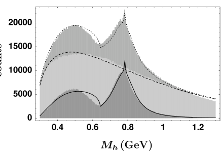
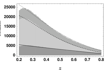
(a)		(b)

Figure 4: Semi-inclusive dihadron counts from the PYTHIA event generator Sjostrand et al. (2001) tuned for HERMES Liebing (2004) and results of the fit (a) as a function of $M_{h}$, (b) as a function of $z$. Solid line: $p$-wave contribution; dashed line: $s$-wave contribution; dotted line: sum of the two. The contributions of the $\eta$ and $K^{0}$ have been excluded.

The values of the parameters obtained by the fit are:

$$\alpha_{s} =2.60\pm 0.05\;\text{GeV}^{2}, \beta_{s} =-0.751\pm 0.008, \gamma_{s} =-0.193\pm 0.004,$$ (32)

$$\alpha_{p} =7.07\pm 0.11\;\text{GeV}^{2}, \beta_{p} =-0.038\pm 0.003, \gamma_{p} =-0.085\pm 0.004,$$ (33)

$$f_{s} =1197\pm 2\;\text{GeV}^{-1}, f_{\rho} =93.5\pm 1.6, f_{\omega} =0.63\pm 0.03,$$ (34)

$$f^{\prime}_{\omega} =75.2\pm 1.2, M_{s} =(2.97\pm 0.04)\,M_{h}.$$ (35)

The coupling constants are fixed modulo an overall normalization factor which depends on the luminosity and is irrelevant for asymmetry calculations. The sign of the coupling constants is also not fixed, but the relative sign of $f_{\rho}$, $f_{\omega}$ and $f^{\prime}_{\omega}$ is (see below).

In the $p$-wave channel, our model deviates significantly from the generated spectrum in the region around 0.6 GeV, substantially increasing the $\chi^{2}$. This is due to the interference between channels 2 and 4, which is not included in the Monte Carlo generator. At the same time, in the $s$-channel the curve obtained from our model underestimates the data in the same region. Thus, the sum of the two curves is in good agreement with the total generated spectrum, to which the Monte Carlo generator is actually tuned. The agreement would be improved further if the contribution of the $\omega$ were extended at higher invariant masses by leaving the narrow-width approximation for the $\omega$ resonance and smearing the step function in Eq. (28). Note that the interference is in this case constructive because the signs of the couplings $f_{\rho}$ and $f^{\prime}_{\omega}$ have been taken equal. If the two couplings were taken opposite, then a destructive interference would take place and the model would underestimate the $p$-wave data at around 0.6 GeV. The agreement with the total spectrum would then be worsened. Also the $f_{\omega}$ coupling has been taken to have the same sign of $f_{\rho}$ to avoid destructive interference patterns. It is difficult with the present poor knowledge to make any conclusive statement about $\rho$-$\omega$ interference in semi-inclusive dihadron production. However, we can at least conclude that in our model the best agreement with the event generator is achieved when the three couplings $f_{\rho}$, $f_{\omega}$ and $f^{\prime}_{\omega}$ have the same sign.

V Predictions for polarized fragmentation functions and transverse-spin asymmetry

Using the parameters obtained from the fit we can plot the results for the fragmentation functions $D_{1,ll}$, $H_{1,ot}^{{<\kern-2.10002pt{\scriptscriptstyle)}}}$, and $D_{1,ol}$. The function $D_{1,ll}$ is a pure $p$-wave function. It depends on $|F^{p}|^{2}$, the modulus square of Eq. (28), and has a behavior very similar to $D_{1,oo}^{p}$, the $p$-wave part of $D_{1,oo}$. In Fig. 5 (a) we plot the ratio between $D_{1,ll}$ and $D_{1,oo}$, integrated separately over $0.2<z<0.8$. In Fig. 5 (b) we plot the same ratio but with the two functions multiplied by $2M_{h}$ and integrated over $0.3\,\text{GeV}<M_{h}<1.3\,\text{GeV}$. In the same figures, the dotted lines represent the positivity bound Bacchetta and Radici (2003)

$$-\frac{3}{2}\,D_{1,oo}^{p}\leq D_{1,ll}\leq 3D_{1,oo}^{p}.$$ (36)

(a)		(b)

Figure 5: Model prediction for the ratio $D_{1,ll}/D_{1,oo}$: (a) as a function of $M_{h}$, (b) as a function of $z$. The dotted lines represent the positivity bounds of Eq. (36).

The functions $D_{1,ol}$ and $H_{1,ot}^{{<\kern-2.10002pt{\scriptscriptstyle)}}}$ arise from the interference of $s$ and $p$ waves, i.e. from the interferences of channels 1-2, 1-3, and 1-4, proportional to the product $(f_{s}\,f_{\rho})$, $(f_{s}\,f_{\omega})$, $(f_{s}\,f^{\prime}_{\omega})$, respectively. Since the relative sign of $f_{s}$ and the $p$-wave couplings is not fixed by the fit, we can only predict these functions modulo a sign. For the plots, we assume that the $p$-wave couplings have a sign opposite to $f_{s}$ (as suggested by the sign of preliminary HERMES data van der Nat (2005)).

In Fig. 6 (a) we plot the ratio between $-|\vec{R}|/M_{h}\,H_{1,ot}^{{<\kern-2.10002pt{\scriptscriptstyle)}}}$ and $D_{1,oo}$, integrated separately over $0.2<z<0.8$. In Fig. 6 (b) we plot the same ratio but with the two functions multiplied by $2M_{h}$ and integrated over $0.3\,\text{GeV}<M_{h}<1.3\,\text{GeV}$. In the same figures, the dotted lines represent the positivity bound Bacchetta and Radici (2003)

$$\frac{|\vec{R}|}{M_{h}}\,H_{1,ot}^{{<\kern-2.10002pt{\scriptscriptstyle)}}}\leq\sqrt{\frac{3}{8}\,D_{1,oo}^{s}\left(D_{1,oo}^{p}-\frac{1}{3}\,D_{1,ll}\right)}.$$ (37)

(a)		(b)

Figure 6: Model prediction for the ratio $(-|\vec{R}|\,H_{1,ot}^{{<\kern-2.10002pt{\scriptscriptstyle)}}})/(M_{H}\,D_{1,oo})$: (a) as a function of $M_{h}$, (b) as a function of $z$. The overall sign of $H_{1,ot}^{{<\kern-2.10002pt{\scriptscriptstyle)}}}$ cannot be predicted by the model and is chosen to have an agreement with the sign of preliminary HERMES measurements van der Nat (2005). The dotted lines represent the positivity bounds of Eq. (37).

As is evident, there are two main contributions:

• the interference between channel 1 ($s$-wave background) and the imaginary part of 2 ($\rho$ resonance), with a shape peaked at the $\rho$ mass, i.e. roughly proportional to the imaginary part of the $\rho$ resonance in Eq. (28);

• the interference between channel 1 ($s$-wave background) and 4 ($\omega$ resonance decaying into three pions), with a shape peaked at $M_{h}\approx 0.5$ GeV, roughly proportional to the third (imaginary) term in Eq. (28).

The two contributions have comparable size and are large. At this point, we want to stress once more that our model assumptions imply that the above channels can interfere in a complete way, since the spectators $X_{1}$, $X_{2}$ and $X_{4}$ are the same. As already argued before, it is likely that only a fraction of the $X_{2}$ and $X_{1}$ states interfere, and so does a (in general different) fraction of the $X_{4}$ and $X_{1}$ states. This could decrease the sizes of the two “peaks” of Fig. 6 (a) and accordingly the overall size of the curve in Fig. 6 (b). This is beyond the reach of our model in its present form, but could be a way to proceed when fitting data related to $H_{1,ot}^{{<\kern-2.10002pt{\scriptscriptstyle)}}}$.

In Fig. 7 (a) we plot the ratio between $-D_{1,ol}$ and $D_{1,oo}$, integrated separately over $0.2<z<0.8$. In Fig. 7 (b) we plot the same ratio but with the two functions multiplied by $2M_{h}$ and integrated over $0.3\,\text{GeV}<M_{h}<1.3\,\text{GeV}$. The dotted line in Fig. 7 (a) represents the positivity bound Bacchetta and Radici (2003) (in the second plot the bound lies beyond the plot range)

$$D_{1,ol}\leq\sqrt{\frac{3}{4}\,D_{1,oo}^{s}\left(D_{1,oo}^{p}+\frac{2}{3}\,D_{1,ll}\right)}.$$ (38)

(a)		(b)

Figure 7: Model prediction for the ratio $-D_{1,ol}/D_{1,oo}$: (a) as a function of $M_{h}$, (b) as a function of $z$. The overall sign of $D_{1,ol}$ depends on the choice made on the sign of $H_{1,ot}^{{<\kern-2.10002pt{\scriptscriptstyle)}}}$. The dotted lines represent the positivity bounds of Eq. (38).

In this case, the function $D_{1,ol}$ receives basically only one contribution, namely from the interference between channel 1 ($s$-wave background) and the real part of 2 ($\rho$ resonance). In fact, its shape has a sign change at the $\rho$ mass and is roughly proportional to the real part of the $\rho$ resonance in Eq. (28). Channel 3 is negligible as in the previous case, while channel 4 plays no role now because we assumed it to be purely imaginary.

Next we compute the asymmetry defined in Eq. (18), integrated over all variables but one. In Fig. 8 (a) we plot

$$A_{UT}^{\sin(\phi_{R}+\phi_{S})}(M_{h})=c\;\frac{\int_{0.2}^{0.8}dz\;|\vec{R}|/M_{h}\;H_{1,ot}^{{<\kern-2.10002pt{\scriptscriptstyle)}}}(z,M_{h}^{2})}{\int_{0.2}^{0.8}dz\;D_{1,oo}(z,M_{h}^{2})},$$ (39)

and in Fig. 8 (b) we plot

$$A_{UT}^{\sin(\phi_{R}+\phi_{S})}(z)=c\;\frac{\int_{0.5}^{1}dM_{h}\;2M_{h}\;|\vec{R}|/M_{h}\;H_{1,ot}^{{<\kern-2.10002pt{\scriptscriptstyle)}}}(z,M_{h}^{2})}{\int_{0.5}^{1}dM_{h}\;2M_{h}\;D_{1,oo}(z,M_{h}^{2})},$$ (40)

where

$$c=\frac{\pi}{4}\,\frac{\int_{0.1}^{0.85}dy\;\int_{x_{\text{min}}}^{x_{\text{max}}}dx\;\frac{1-y-y^{2}\,\gamma^{2}/4}{x\,y^{2}\,(1+\gamma^{2})}\;\bigr{[}4\,\bigr{(}h_{1}^{u}(x)-h_{1}^{\bar{u}}(x)\bigl{)}+\bigr{(}h_{1}^{\bar{d}}(x)-h_{1}^{d}(x)\bigl{)}\bigl{]}}{\int_{0.1}^{0.85}dy\;\int_{x_{\text{min}}}^{x_{\text{max}}}dx\;\frac{1-y+y^{2}/2+y^{2}\,\gamma^{2}/4}{x\,y^{2}\,(1+\gamma^{2})}\;\bigr{[}4\,\bigr{(}f_{1}^{u}(x)+f_{1}^{\bar{u}}(x)\bigl{)}+\bigr{(}f_{1}^{\bar{d}}(x)+f_{1}^{d}(x)\bigl{)}\bigl{]}}.$$ (41)

We neglected strange quark contributions. The fact that the $d$ and $\bar{u}$ transversity distributions enter with an opposite sign is due to the symmetry properties of the fragmentation functions. As already discussed in Sec. III, the fragmentation function $H_{1,ot}^{{<\kern-2.10002pt{\scriptscriptstyle)}}}$ is the same for all quarks, but the sign of $\sin(\phi_{R}+\phi_{S})$ changes for $d$ and $\bar{u}$.

In Fig. 8 (c) we plot

$$A_{UT}^{\sin(\phi_{R}+\phi_{S})}(x)=c^{\prime}\;\frac{\int_{y_{\text{min}}}^{0.85}dy\;\frac{1-y-y^{2}\,\gamma^{2}/4}{y^{2}\,(1+\gamma^{2})}\;\bigr{[}4\,\bigr{(}h_{1}^{u}(x)-h_{1}^{\bar{u}}(x)\bigl{)}+\bigr{(}h_{1}^{\bar{d}}(x)-h_{1}^{d}(x)\bigl{)}\bigl{]}}{\int_{y_{\text{min}}}^{0.85}dy\;\frac{1-y+y^{2}/2+y^{2}\,\gamma^{2}/4}{y^{2}\,(1+\gamma^{2})}\;\bigr{[}4\,\bigr{(}f_{1}^{u}(x)+f_{1}^{\bar{u}}(x)\bigl{)}+\bigr{(}f_{1}^{\bar{d}}(x)+f_{1}^{d}(x)\bigl{)}\bigl{]}},$$ (42)

where

$$c^{\prime}=\frac{\pi}{4}\,\frac{\int_{0.2}^{0.8}dz\;\int_{0.5}^{1}dM_{h}\;2M_{h}\;|\vec{R}|/M_{h}\;H_{1,ot}^{{<\kern-2.10002pt{\scriptscriptstyle)}}}(z,M_{h}^{2})}{\int_{0.2}^{0.8}dz\;\int_{0.5}^{1}dM_{h}\;2M_{h}\;D_{1,oo}(z,M_{h}^{2})}.$$ (43)

(a)		(b)		(c)

Figure 8: $A_{UT}^{\sin(\phi_{R}+\phi_{S})}$ moment defined in Eq. (18) at HERMES kinematics for a proton target: (a) as a function of $M_{h}$, (b) as a function of $z$, (c) as a function of $x$. The different lines correspond to different models of the transversity distribution function: dotted line from Ref. Wakamatsu (2001), dash-dotted line from Ref. Korotkov et al. (2001), dashed line from Ref. Schweitzer et al. (2001), solid line from Ref. Soffer et al. (2002).

The choices of the integrations boundaries for $x$, $y$, $z$ and $M_{h}$ are inspired by the HERMES cuts van der Nat (2005). We took ($s=56.2$ GeV²)

$$x_{\text{min}} =\text{Max}\bigl{[}0.023,Q^{2}_{\text{min}}/\bigl{(}y(s-M^{2})\bigr{)}\bigr{]},$$ (44)

$$x_{\text{max}} =\text{Min}\bigl{[}0.4,1-(W^{2}_{\text{min}}-M^{2})/\bigl{(}y(s-M^{2})\bigr{)}\bigr{]},$$ (45)

$$y_{\text{min}} =\text{Max}\bigl{[}0.1,Q^{2}_{\text{min}}/\bigl{(}x(s-M^{2})\bigr{)},(W^{2}_{\text{min}}-M^{2})/\bigl{(}(1-x)(s-M^{2})\bigr{)}\bigr{]}.$$ (46)

For the unpolarized parton distribution functions we take the parameterization of Ref. Gluck et al. (1998). For the transversity distribution function, we take the estimates of Refs. Wakamatsu (2001); Korotkov et al. (2001); Schweitzer et al. (2001); Soffer et al. (2002). The sign of the preliminary data indicates that the $s$-wave and $p$-wave couplings should have opposite signs and thus $H_{1,ot}^{{<\kern-2.10002pt{\scriptscriptstyle)}}}$ should be negative. The asymmetry obtained from our model appears to overestimate the preliminary HERMES data van der Nat (2005) by about a factor 3-4. This probably indicates that the model overestimates in general the effect of interferences. Apart from the overall normalization, the height of the bump around $M_{h}\approx 0.5$ GeV seems to be too big relative to the $\rho$ peak, which is probably due to the fact that not all the $\pi^{+}\pi^{-}$ pairs in channel 4 should be considered in $p$ wave. However, in order to make more conclusive statements it is necessary to wait for HERMES final data. Obviously, it would be better to compare our model with an observable where $H_{1,ot}^{{<\kern-2.10002pt{\scriptscriptstyle)}}}$ can be isolated, e.g., in $e^{+}e^{-}$ annihilation at BELLE Hasuko et al. (2003).

In Fig. 9 we plot the same asymmetry as before, but for the kinematics of the COMPASS experiment. We assumed the same cuts as before and change only the value of $s$. The size of the $M_{h}$- and $z$-dependent asymmetries is smaller than at HERMES. This is due to the sensitivity of COMPASS to lower values of $x$, where models predict transversity to be small, while the unpolarized distribution functions are big. Due to the same reason, there is a much larger difference among the models, as they differ substantially at low $x$. The asymmetries could be enhanced if the low-$x$ region is excluded from the integration.

(a)		(b)		(c)

Figure 9: $A_{UT}^{\sin(\phi_{R}+\phi_{S})}$ moment defined in Eq. (18) at COMPASS kinematics for a proton target: (a) as a function of $M_{h}$, (b) as a function of $z$, (c) as a function of $x$. The different lines correspond to different models of the transversity distribution function: dotted line from Ref. Wakamatsu (2001), dash-dotted line from Ref. Korotkov et al. (2001), dashed line from Ref. Schweitzer et al. (2001), solid line from Ref. Soffer et al. (2002).

The COMPASS collaboration has also presented preliminary data of the above asymmetry for a deuteron target Martin (2006). We plot our prediction in Fig. 10. The different isospin structure of the target, combined with that of the fragmentation functions in our model, decreases the asymmetry. The $x$-dependent asymmetry is less than half of that for the proton target, while the $M_{h}$- and $z$-dependent asymmetries are about 10 times smaller than for the proton target.

(a)		(b)		(c)

Figure 10: $A_{UT}^{\sin(\phi_{R}+\phi_{S})}$ moment defined in Eq. (18) at COMPASS kinematics for a deuteron target: (a) as a function of $M_{h}$, (b) as a function of $z$, (c) as a function of $x$. The different lines correspond to different models of the transversity distribution function: dotted line from Ref. Wakamatsu (2001), dash-dotted line from Ref. Korotkov et al. (2001), dashed line from Ref. Schweitzer et al. (2001), solid line from Ref. Soffer et al. (2002).

VI Conclusions

In this paper we presented a model for the process $q\to\pi^{+}\pi^{-}X$ at invariant mass $M_{h}\lesssim 1.3$ GeV. We used a “spectator” model, where the sum over all possible intermediate states $X$ is replaced by an effective on-shell state. Using this model we calculated the fragmentation functions that can be defined at leading twist when considering only relative $s$ and $p$ waves of the pion pair Bacchetta and Radici (2003). We obtained nonzero results for four out of five of them.

We fixed the values of the parameters of the model by comparing the unpolarized fragmentation function $D_{1,oo}$ with the output of the PYTHIA event generator Sjostrand et al. (2001) tuned for HERMES Liebing (2004). The main characteristics of the $M_{h}$ and $z$ shapes of $D_{1,oo}$ are qualitatively well described.

We made predictions for the fragmentation functions $D_{1,ll}$, $D_{1,ol}$, and $H_{1,ot}^{{<\kern-2.10002pt{\scriptscriptstyle)}}}$. The first one is a pure $p$-wave function, it is found to be positive, about 50% of the unpolarized fragmentation function and with peaks at the $\rho$ mass and at around $M_{h}\approx 0.5$ GeV, where the $\omega$ decaying into three pions gives a large contribution.

The function $D_{1,ol}$ arises from the interference between $s$ and $p$ wave. Since in our model we assumed the $s$ wave to be purely real, this function turns out to be proportional to the real part of the $p$ wave and in particular displays a sign change at the $\rho$ mass. The size of the function is small, in particular when integrated over the invariant mass, due to the sign change. Our model cannot predict the overall sign of the function.

The function $H_{1,ot}^{{<\kern-2.10002pt{\scriptscriptstyle)}}}$ also arises from the interference between $s$ and $p$ waves, but is proportional to the imaginary part of the $p$ wave, i.e., it has peaks at the $\rho$ mass and at around $M_{h}\approx 0.5$ GeV, due to the contribution of the $\omega\to 3\pi$ channel. Its size is about 30% of the unpolarized fragmentation function. Our model cannot predict the overall sign of the function.

The function $H_{1,ot}^{{<\kern-2.10002pt{\scriptscriptstyle)}}}$ is of particular interest because in two-hadron-inclusive deep inelastic scattering off transversely polarized targets it gives rise to a single-spin asymmetry in combination with the transversity distribution function. Therefore, it could be used as an analyzer for this so far unknown distribution function. We estimated this single-spin asymmetry at HERMES kinematics using four different models for the transversity distribution function. We found the asymmetry to be of the order of 10% on average. The sign of the preliminary HERMES measurements suggests that $H_{1,ot}^{{<\kern-2.10002pt{\scriptscriptstyle)}}}$ should be negative. The measurement indicates that the asymmetry in our model is about 3-4 times bigger than the data. This probably means that our model overestimates the effects of interferences. However, final experimental results are needed to make more reliable comparisons.

For COMPASS kinematics, the enhanced sensitivity to the portion of phase space at very low $x$ induces a reduction in the spin asymmetry with respect to HERMES, which can largely differ depending on the model for transversity. For the deuteron target, the particular isospin structure, combined with that of the fragmentation functions in our model, induces a further reduction such that the resulting asymmetry is much smaller than for the proton, in agreement with preliminary data of the COMPASS collaboration.