Solution of Dynamical Chiral Symmetry Breaking in Minkowski Space
Linearized approximation

Abstract

Chiral symmetry breaking and mass generation is studied in a vectorial, confining asymptotic free gauge theory. Using the Schwinger-Dyson equation in improved ladder approximation, we calculate the fermion propagator in the whole Minkowski space. The estimate for $f_{\pi}$ and the dependence of physical mass on a coupling strength is provided. We focus on the extraction of spectral function of fermion propagator in the strongly coupled regime. Our calculations indicate that up to the crossover between walking and QCD-like running dynamics, the real pole of the propagator is not excluded and very likely it is actually developed at zero temperature theory.

I Introduction

Chiral symmetry plays a crucial role in particle physics. Our recent understanding of low energy $E\simeq\Lambda_{QCD}$ hadron physics is heavily based on this phenomenon. The observed pions are naturally identified with the approximatively massless Nambu-Goldstone modes of broken $SU(2)_{L}\times SU(2)_{R}$ chiral symmetry. The associated quark mass generation is driven by the QCD strong interaction of light quarks via the colored gauge boson of $SU(3)_{c}$ Yang-Mills theory. Although experimentally observable small current masses enter the QCD Lagrangian, the huge amount of constituent quark mass is generated dynamically.

There are also interesting proposals to solve hierarchy problem of the Standard Model without point-like Higgs, which invoke strong interactions. They include Technicolor models FASUS1981 , Topcolor assisted Technicolor models TOPCOLOR , Extended Technicolor Models DISU1979 ; EILA1980 with walking effective coupling HOLDOM1985 and even the extradimensional one GHTY2002 . In realistic versions of models, the part of the chiral group is a subgroup of standard model $SU(2)_{w}\times U(1)_{Y}$, while the breaking of chiral symmetry automatically implies spontaneous electroweak symmetry breaking. Hence these models are very ambitious, as they should explain the observed masses of fermions, but they must give the correct masses to $W^{\pm},Z$ as well. For a rather recent review of electroweak symmetry breaking in Technicolors see REWIEV .

In the above mentioned models the particles masses are mostly (if not fully) generated via loops. If the coupling constant is small enough we can say that the chiral symmetry plays the role of ’custodial symmetry’ which prevents the particle from receiving a mass. Hence relatively strong coupling is needed, the dynamical fermion mass generation is therefore intrinsically non-perturbative phenomenon of quantum field theory. There are some challenging problems connected to the singularity structure of Green’s functions in strong coupling models like QCD or Technicolors: e.g., questions about the presence and the position of propagator poles. In view of recent achievements in lattice calculations and in numerical results obtained by employing Schwinger-Dyson equations in the Euclidean space, solutions obtained in the the whole Minkowski space should bring new insights for these models.

Let us mention some background and related work. The gap equations have been used for many years to study spontaneous chiral symmetry breaking in field theories SCALING ; GAUGE ; KLUCI ; CHIRALY ; HAKUYA2005 Solving the Schwinger-Dyson equation directly in Minkowski space has an advantage of providing the solution also for timelike momenta, which are not directly accessible in Euclidean formalism. Up to date, only few attempts or suggestions BICUDO ; ADBISA ; ARRBRO2003 ; BLUJOH1998 to solve the problem of dynamical chiral symmetry breaking in the whole Minkowski space are known. In our presented approach, we assume and employ dispersion relation for the dynamical mass function $\Sigma$. However we should note that the resulting integral representation for the fermion propagator cannot be identified with the standard Lehmann spectral representation. Thus giving up the assumption of a Lehmann spectral representation for propagator, which seems to be unavoidable due to the high momentum asymptotic of the fermion correlators, we obtain perfectly stable solutions even far away from the chiral phase transition. We compare our Minkowski solutions with ones obtained independently in Euclidean space.

The paper is organized as follows. In the next section we will introduce the model and formalism, in section III we explain the solution of gap equation in Minkowski space, in section IV we will check the linear approximation employed. In section V physical scaling law will be provided, i.e., the dependence of the pole mass on the coupling. We discuss further possible progress in the Conclusion and Outlook.

II Toy model and basic formalism

As our toy model consists of just one interacting quark, there is just one massless pion associated with broken chiral symmetry $U(1)\times U(1)/U(1)$. Once the chiral symmetry is spontaneously broken, the massless pole appears in the fermion-boson vertices and the associated current of broken generator induced non-zero transition between vacuum and the pion itself. In that case the pion decay constant

$$<0|j_{5}^{\sigma}(0)|\pi(k)>=if_{\pi}k^{\sigma}$$ (1)

can be estimated by the Pagels-Stokar formula PASTO

$$f_{\pi}^{2}=-4iN_{c}\int\frac{d^{4}p}{(2\pi)^{4}}\frac{\Sigma(p^{2})}{(p^{2}-\Sigma^{2}(p^{2}))^{2}}\left[\Sigma(p^{2})-\frac{p^{2}}{2}\frac{d\Sigma(p^{2})}{dp^{2}}\right]\,,$$ (2)

where $\Sigma$ is mass function defined through the fermion propagator:

$$S(p)=\frac{Z}{\not p-\Sigma(p^{2})}\,.$$ (3)

wherein we take renormalization wave function $Z(p)=1$ from now since its momentum dependence is unimportant in Landau gauge which we will use in our calculation.

The basic input into the relation for the pion decay constant is the dynamical mass $\Sigma$, which we shall assume here to satisfy the dispersion relation:

$$\Sigma(p^{2})=\int\limits_{0}^{\infty}d\omega\,\frac{\rho(\omega)}{p^{2}-\omega+i\epsilon}\,.$$ (4)

In that case we approximate the $\Sigma^{2}$ in the denominator of $S$ by the pole value $m^{2}$, i.e.

$$S=\frac{\not p+\Sigma(p^{2})}{p^{2}-\Sigma^{2}(p^{2})}\rightarrow\frac{\not p+\int\limits_{0}^{\infty}d\omega\,\frac{\rho(\omega)}{q^{2}-\omega+i\epsilon}}{p^{2}-m^{2}+i\epsilon}$$ (5)

where the pole mass is determined self-consistently as

$$\Sigma(m^{2})=m\,.$$ (6)

As we will see in the next section the determination of the function $\rho$ and physical mass $m$ is not difficult task in our denominator approximation.

The dynamical mass is approximately constant function in the infrared $p^{2}<\Lambda$, while it decreases like power of momentum

$$\Sigma\simeq\frac{1}{p^{2}}$$ (7)

for $p^{2}>>\Lambda^{2}$ in an asymptotic free theory characterized by the logarithmically behaving running coupling above the scale $\Lambda$. Recall the QCD scaling here: $E\simeq\Lambda_{QCD}(=400MeV)\simeq\Sigma(0)(=350MeV)\simeq 4f_{\pi}$. In our model the selfenergy behaviour (7) is achieved a bit faster as a consequence of the used Pauli-Villas regulator. When $\Sigma$ approaches $\Lambda$, then $\Lambda$ represents the confinement scale WITTEN and confinement goes hand by hand with the spontaneous chiral symmetry breaking. Unfortunately, the denominator approximation method of this paper are then no longer useful in this case. Nevertheless, the proposed denominator approximation should be rather good CHIRALY for walking (slowly running) theories when $m^{2}<<\Lambda^{2}$.

Here, a short but important digression is in order. Clearly, the propagator given by formula (5) exhibits a real-value pole. This gives rise the natural question of using a Lehmann representation (see the first two formulas in the Appendix) for this purpose. This has been attempted in the paper ADBISA wherein it was found that a spectral representation with a single real pole part explicitly divided is applicable only with crude restrictions. Indeed, it gives reliable result only up to the scale $\Lambda$ and for the couplings which are very close to the critical value $\alpha_{c}$. It seems that $1/p^{2}$ behaviour of the $TrS(p)$ (Tr is taken over the Dirac indices) is dictated too strongly by Lehmann representation, which contradicts $1/p^{4}$ of $TrS(p)$ decrement typically found in the Euclidean space studies. It was also shown in ADBISA that the propagator looses its assumed analytical property in this case. It is stated without proof here, that the ultraviolet asymptotic of the correlators strongly suggest the absence of Lehmann representation for propagators in models with the dynamical chiral symmetry breaking. Perhaps and with great care, the Lehmann representation can be used as a low energy approximation.

In addition we neglect the terms with the derivatives and substitute our integral Ansatz (5) into the Pagels-Stokar formula (2) for the pion decay constant. Doing this explicitly we get

$$f_{\pi}^{2}=-4iN_{c}\int_{0}^{\infty}dx_{1}dx_{2}\int\frac{d^{4}p}{(2\pi)^{4}}\frac{\rho(x_{1})\rho(x_{2})}{(p^{2}-m^{2})^{2}(p^{2}-x_{1}^{2})(p^{2}-x_{2}^{2})}.$$ (8)

After the momentum integration we arrive into the following formula:

$$f_{\pi}^{2}=-\frac{N_{c}}{4\pi^{2}}\int_{0}^{\infty}dx_{1}dx_{2}\frac{\rho(x_{1})\rho(x_{2})}{x_{1}-x_{2}}\left[\frac{\ln{(m^{2}/x_{1})}}{x_{1}^{2}-m^{2}}-\frac{\ln{(m^{2}/x_{2})}}{x_{2}^{2}-m^{2}}\right]$$ (9)

This can be further approximated since one can easily recognize that up to the presence of log’s the double integral factorizes and turns to be square of the pole masses $m^{2}$ exactly. For this estimate we approximate slowly varying log’s in (9)by a constant $K=\ln{(m^{2}/x_{max})}$ where $x_{max}$ is the position of $|\rho|$ function global maximum. Anticipating the typical behaviour of $|\rho|$ it ’explodes’ from the threshold where it is zero to its maximum which lies not so far. Doing this explicitly and using (6) we immediately get:

$$\frac{f_{\pi}}{m}=\frac{\sqrt{KN_{c}}}{2/\pi}\,.$$ (10)

Numerically $K\simeq 0.5$ when $\Sigma(0)\simeq\Lambda$ which by about 50 percentage underestimates an experimentally well tested QCD result. It is not so bad estimate because of denominator approximation, Eq. (9) represents at least an interesting formula which relates the physical pole mass $m$, the absorptive part of dynamical mass function $\rho$ and the decay constant of the Nambu-Goldstone boson. Finally notice that it is impossible to obtain such result within the use of Lehmann representation since the formula appears to be ultraviolet divergent in that case.

Of course, in any case $f_{\pi}$ can be calculated purely from the Wick rotated results on $\Sigma$ (see Appendix ) and this is not clearly a manifest quantity where the knowledge of the timelike structure of the propagator is necessary. Various timelike form factors are the right possible cases. To be able to calculate them from first principles in QCD the nonperturbative knowledge of $\Sigma$ in the whole Minkowski is required.

The vectorial interaction with gluons leads to the gap equation which in the Landau gauge and one skeleton loop approximation reads

$$\Sigma(p^{2}) = -ig^{2}C_{2}(R)\int\frac{d^{4}q}{(2\pi)^{4}}\gamma_{\alpha}\left[-g^{\alpha\beta}+\frac{(p-q)_{\alpha}(p-q)_{\beta}}{(p-q)^{2}}\right]\,G(p-q)S(q)\gamma_{\beta}\,.$$ (11)

where $C_{2}(R)=(N^{2}-1)/2N$ for fermions in fundamental representation of SU(N). To implement the running coupling, a very simple Ansatz for the product of gluon and vertex form factors has been used in ADBISA . It was chosen such that for a large Euclidean momenta such running coupling $\alpha_{run}$ behaves like

$$\alpha_{run}(q^{2})\simeq\frac{\alpha_{run}(0)}{1+\frac{q^{2}}{\Lambda^{2}}}$$ (12)

which is continuous modification of sharp cutoff used in a recent studies KURACHI2006 .

Implementation of $\alpha_{run}$ is easily achieved by adding negative term to the usual boson propagator,i.e.

$$G(l)=\frac{1}{q^{2}-m_{g}^{2}+i\epsilon}-\frac{1}{q^{2}-{\Lambda}^{2}+i\epsilon}$$ (13)

in Eq. (11) where we have introduced also an effective gauge boson mass $m_{g}$.

Further note, that we prefer to have only one dominant scale and we do not attempt to solve the model in all its possible peculiar phases. For this purpose we fix the ratio such that

$$\frac{\Lambda^{2}}{m_{g}^{2}}=10\,.$$ (14)

Throughout this paper we will express the dimensionfull quantities in the units of $m_{g}=1$ and/or $\Lambda$ if stated explicitly.

Let us stressed at the end of this section that the scale $\Lambda$ mimic $\Lambda_{Q}CD$ or characteristic scale of an asymptotic free gauge theory and it has nothing to do with the renormalization/regularization procedure which does not take place here. Asymptotic freedom is necessary condition which make our calculation meaningful. In the real QCD the high energy modes are damped by logarithm which is the main difference here. As we will see, the running (or walking) of the effective coupling largely affects the asymptotic behaviour of the fermion mass function, it behaves like $1/p^{4}$ while the mass of chiral quarks behaves like $1/p^{2}$ for $p^{2}>>\Lambda^{2}_{QCD}$

III Solving gap equation for $\rho$

The simple integral representation Ansatze allows us to convert the complicated equations with singular kernel to the real regular equation for the function $\rho$. The key point is the analytical momentum integration in the gap equation with self-consistent arrival to the desired dispersion relation, i.e., into the form of propagator which we have assumed and from which we have started the calculation. The only assumption we need is the uniqueness of the dispersion for $\rho$.

Applying the trivial algebraic identity on integral representation of $S$

$$\int dx\frac{\rho(x)}{(q^{2}-x+i\epsilon)(q^{2}-m^{2}+i\epsilon)}=\int dx\frac{\rho(x)}{(m^{2}-x)}\left[\frac{1}{q^{2}-m^{2}+i\epsilon}-\frac{1}{q^{2}-x+i\epsilon}\right]$$ (15)

and abstracting from various prefactors, the integral kernel reduces to the differences of one loop perturbation theory integrals, each of them being regularized by Pauli-Villars. Consequently we can immediately use this result.

The momentum integration is very straightforward since it follows standard tricks. E.g., the Feynman parameterization is a convenient way to perform it explicitly. At the end the Feynman parameter is converted into the integration variable of an appropriate dispersion relation. The integral is finite and does not require any subtractions as it must in the theory without explicit mass term. For convenience, the relevant formula can be found for instance in the paper LACO or in any standard textbook.

Hence after substituting the integral Ansatz (5) into the gap equation, making a trace and integrating over the momentum it leads to the following expression for the dynamical mass:

$$\Sigma(p^{2}) = \int d\omega\frac{\rho(\omega)}{p^{2}-\omega+i\epsilon}\,,$$

$$\rho(\omega) = \frac{\alpha^{*}}{(4\pi)}\int dx\frac{\rho(x)}{m^{2}-x}\left[X_{0}(\omega;m_{g}^{2},m^{2})-X_{0}(\omega;{\Lambda}^{2},m^{2})\right.$$ (16)

$$- \left.X_{0}(\omega;m_{g}^{2},x)+X_{0}(\omega;{\Lambda}^{2},x)\right]\,,$$

$$X_{0}(\omega;a,b) = \frac{\sqrt{(\omega-a-b)^{2}-4ab)}}{\omega}\Theta\left(\omega-(\sqrt{a}-\sqrt{b})^{2}\right)\,,$$ (17)

where $\Theta$ represents for the usual Heaviside step function and we use following shorthand notation:

$$\alpha^{*}=\frac{C_{2}(R)g^{2}}{4\pi}.$$ (18)

Assuming of uniqueness DR the Eq. (16) represents a homogeneous integral equation to be solved. The Eq. (III) has a regular kernel. In general the homogeneous equation needs a suitable ’normalization condition’. Here this can be easily identified with the condition of on-shellness (6), i.e.

$$\int_{(m_{g}+m)^{2}}^{\infty}dx\frac{\rho(x)}{m^{2}-x}=m$$ (19)

where we have explicitly indicated the branch point as dictated by the arguments of step functions in (16). Using Rel. (19), the equation to be actually solved numerically now reads:

$$\rho(\omega) = \frac{\alpha^{*}}{(4\pi)}\left[m\left(X_{0}(\omega;m_{g}^{2},m^{2})-X_{0}(\omega;{\Lambda}^{2},m^{2})\right)\right.$$ (20)

$$- \int dx\frac{\rho(x)}{m^{2}-x}\left.\left(X_{0}(\omega;m_{g}^{2},x)-X_{0}(\omega;{\Lambda}^{2},x)\right)\right]\,.$$

Using the method of iterations it is found that the integral equations is perfectly convergent and stable for almost any combinations of $\alpha^{*}$ and $m$ (without imposed (19)). Hence the actual search of the true solution is very straightforward. For a given $\alpha^{*}$ we scan suitably chosen interval of $m$ in such a way that the identity (19) is achieved with required accuracy.

For the purpose of comparison we solve Euclidean gap equation. After the Wick rotation and the angle integration it can be cast into the following form:

$$M(x)=m_{0}+\frac{\alpha^{*}}{8\pi x}\,\int_{0}^{\infty}dy\,M(y)\frac{-m_{g}^{2}+\Lambda^{2}+\sqrt{\lambda(x,y,m_{g}^{2})}-\sqrt{\lambda(x,y,{\Lambda}^{2})}}{y+M^{2}(y)}\,,$$ (21)

where the positive variables $x=p_{E}^{2}=-p^{2},y=q^{2}_{E}=-q^{2}$ and the dynamical mass is simply $M(x)=\Sigma(p^{2})$. $\lambda$ represents standard Kallen triangle function

$$\lambda(x,y,z)=x^{2}+y^{2}+z^{2}-2xy-2xz-2yz$$ (22)

First, let us discuss the timelike momentum behaviour. The resulting absorptive part of the dynamical mass function starts with negative infinite derivative from a zero at the threshold $\omega^{1/2}=m_{g}+m$ reaching the first most robust peak. Then after going through two additional local maxima (minima) it behaves exactly like

$$\rho(p^{2})\simeq\frac{1}{p^{2}}$$ (23)

for $p^{2}>>\Lambda^{2}$ without any additional oscillation. The resulting mass function is displayed in Fig. 1 for two values of the coupling $\alpha^{*}=4$ and $\alpha^{*}=5$. Most interestingly, to see a detailed behaviour we plot the absolute value of real (dispersive) and absorptive (imaginary) part of the dynamical mass in Fig. 2.

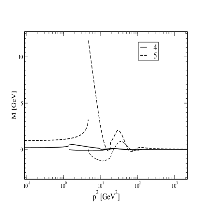
Figure 1: Dynamically generated mass functions at timelike regime. Dashed(solid) line represents the solution for $\alpha^{*}=5$($\alpha^{*}=4$). Thick (thin) line stands for dispersive (absorptive -$\rho$-) part respectively.

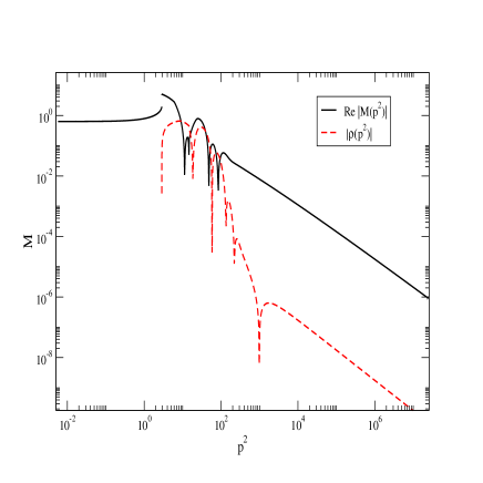
Figure 2: Log-log display of the absolute values of real an imaginary parts of dynamical mass for $\alpha^{*}=5$.

We argue that the observed ”resonant like behaviour” Green’s functions is an inherent property of strong coupling -supercritical- dynamics. That this must be so for higher point Green’s functions due to the formation of hadronic bound states and resonances is an experimental fact and indeed an almost trivial statement in QCD. Recall that the similar thing could happens to propagators of quarks is non-trivial observation. Recall that, this is obtained even without nontrivial inputs from higher order corrections involving mainly the dressed vertices which are connected directly with the physical spectra e.g. the lowest lying meson states $\pi,\rho,\omega,\sigma..$. We should stress at this place that there are only tiny numerical errors ( we use for integration number of 990 Gaussian mesh points in the both cases presented, however using few hundreds with the suitable density is always justified). We mention here also that the principal value integral over the $\rho$ has been calculated analytically, the result of which is presented in the Appendix for completeness. The cancellation among negative and positive contributions in the integral (4) gives the correct -$p^{-2}$ - ultraviolet decreasing log moderated behaviour of the dispersive part of the dynamical mass function.

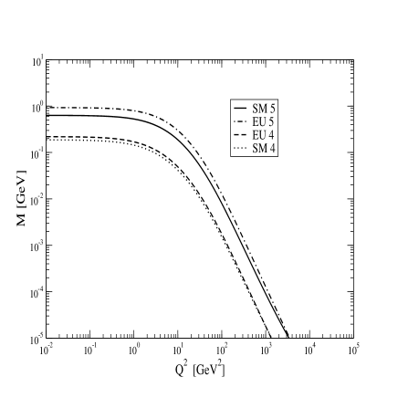
Figure 3: Dynamical mass function in the spacelike regima of momentum. Spectral Minkowski solutions are labeled by SM , the solutions obtained in the Euclidean space are labeled by EU.

The dynamical mass function for the spacelike momenta is displayed in Fig. 3. Being below the branch point the integration washout the oscillating behaviour and the dynamical mass function is a smooth function. We can see in Fig. 3 that not so far from the critical coupling $\alpha_{c}^{*}=3.8$ Minkowski and Euclidean results reasonably agree with each other. The numerical results of our studies point towards an analytical structure of the ’quark’ propagator with a real pole and branch point singularity on the real axis. Close to the chiral phase transition, the suggested nature of this singularity is determined with good confidence.

The impact of difference between walking and running $SU(N)$ gauge theories has been recently investigated in Refs. KURACHI2006 . Our results give additional information: vanishing difference between Euclidean and Minkowski solution suggests that there are no additional complex singularities in the complex plane of the momenta. In Technicolor slang: in walking theory the fermion propagator singularity is dominated by a real pole and associated particle mode can be unconfined. Disappearance of the real propagator pole would be a certain indication of confinement in any model which is heavily based on the walking behaviour of the coupling constant. Recall the possibility of chiral symmetry breakdown and the absence of confinement is supported by an arguments in CHIRALY .

In Fig. 4 we show the solution for dynamical mass as a function of $\alpha^{*}$.

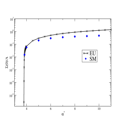
Figure 4: Scaling laws as it is seen in the Euclidean and Minkowski approximations.

In the walking regime $(1-1.1)\alpha_{c}^{*}$ it can be parametrized by the known SCALING ; CHIRALY scaling low

$$\Sigma(0)\simeq C\cdot\Lambda e^{-\left[k(\alpha^{*}/\alpha_{c}^{*}-1)^{-1/2}\right]}\,,$$ (24)

where $C=O(1)$and $k\simeq\pi$ .

Increasing the coupling and leaving thus the walking coupling domain and slowly approaching QCD limit $\Sigma\simeq\Lambda$ a certain discrepancy appears. In present, the nature of the all amount of the discrepancy cannot be determined with confidence. However we point out the main part is due to the linearized approximation (5). The other, more speculative reason, could be that the pole of the propagator, located for subcritical case on the real axis, moves gradually into the complex plan receiving non-negligible imaginary part. Hence the integral representation employed for our calculations would become inappropriate.

IV Checking the approximation (5)

At present we do not know any reason why the spacelike Euclidean calculation should differ from the ’true’ Minkowski space calculation on the real negative axis of four-momentum. Hence the calculation performed in the Euclidean formalism can serve as a good guidance. To observe how much the neglect of a running mass in the denominator (5) affects the behaviour in spacelike domain, we make a similar approximation in the Euclidean space counterpart. For this purpose we replace in Eq. (21) the appropriate part of the propagator follows

$$\frac{M(y)}{y+M^{2}(y)}\rightarrow\frac{M(y)}{y+M^{2}(0)}\,$$ (25)

hoping that $M(0)$ lies sufficiently close to the true pole value $m$. Note, albeit we have estimated $m$ in our Minkowski treatment we cannot use this value, since this is already underestimated just due to the discussed approximation.

The solution is shown in Fig. 5 for $\alpha*=5$.

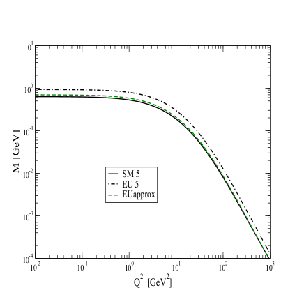
Figure 5: Checking denominator approximation as described in the text. The coupling strength is $\alpha^{*}=5$ and the obtained pole mass is $m=0.695m_{g}$

The corresponding approximation is labeled by the dashed line and much better agreement with the Minkowski approximation is achieved. It leaves little space for other effects and indirectly indicates that the position of propagator singularities actually lies on the real axis. We should mention that the approximation (5) exhibits a similar effect for all studied value of $\alpha^{*}$. On the other side, the splitting of the obtained scaling law functions becomes rather large when $m/\Lambda\simeq 1$. To avoid some speculations we conclude that it simply calls to go beyond the approximation employed.

V Physical scaling law

The pole mass of the propagator can be the only physical observable here. In this section we will largely simplify and speculate. We disregard the systematic error which follows from the approximations and assume the ratio $m/\Sigma(0)$ being reliably estimated. We leave aside the complicated task of confinement-deconfinement-chiral phases WITTEN ; PHASES which lies beyond the scope of this paper and certainly beyond the ability of the toy model used here. We will simply assume that the modeled propagator is a part of the theory in which the singularities of the Green’s functions persist in the S-matrix (That the opposite can happen is well known). In this case the pole mass of the propagator is the only possible physical observable here. In a gauge theory, the value of dynamically generated $m$ cannot be affected by a gauge fixing choice and cannot depend on the associated auxiliary parameters. To make some approximations in the infinite gap equations system is necessary, e.g., the truncation of the equations system, have always some unwanted impact on the calculation scheme (in)dependence. Many studies have investigated this important, but complicated issue. For some discussion in the context of Euclidean Schwinger-Dyson formalism see GAUGE . The value $\Sigma(0)$ is usually believed be an approximately scheme invariant if its value is rather close to the physical $m$. Then there follows important message from the Minkowski study attempted here. We present the physical scaling low in Fig. 6 and compare with the more standard infrared value $\Sigma(0)$.

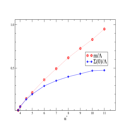
Figure 6: Comparison of physical scaling law with $\Sigma(0)$ in Minkowski approximations.

The observation of large splitting of the lines in Fig. 6 is clear. The ratio $m/\Sigma(0)$ deviates from the save value one rather early. In fact, approximating $m$ by the infrared $\Sigma(0)$ is justified only for slowly running theories.

VI Conclusion and outlook

In the ladder approximation of gap equation with the running coupling modeled by Pauli-Villars regulator we obtain a dynamical mass function in the whole Minkowski space. The momentum space gap equation has been converted to the real regular equation for a real function $\rho$. The procedure is for us surprise perfectly stable for all couplings studied. We compare the solution with the ones obtained in the Euclidean formalism. The employed approximation works rather well for the coupling not so far from the critical one. The Minkowski results appears to be underestimated by about 50 percentage when we get scaling $\Sigma(0)/\Lambda=1$. The physical pole mass has been compared with the infrared one and the physical scaling has been established.

We did not plot the the ratio $f_{\pi}/m$ as a function of $\alpha*(,\Lambda)$. Using a rough estimate by the Pagels-Stokar formula we found that up to deep walking limit this ratio has only weak dependence on the coupling strength $\alpha^{*}$. It decreases from the value $f_{\pi}/m=0.5$ when $\alpha$ is few percentage above $\alpha_{c}^{*}$ to the value 0.25 when $\alpha\simeq 10$ (QCD limit).

The absorptive and dispersive parts of the dynamical mass function are not positive definite functions in the timelike regime, while the later decreases monotonically down in the spacelike regime in a shape already known from the Euclidean studies. The resonant behaviour of Green’s function in the timelike regime can be very inherent to the model with strong coupling, especially for the light quarks in real world QCD. If such behaviour is the reality and general feature of the fermion propagator in chiral breaking phase it calls for a better understanding of its physical impact. The presented toy model hopefully provides a reliable result for slowly running coupling. The application to many questions of electroweak symmetry breaking in Technicolor models is left to a future work. When one moves far away from walking behaviour, one loses a simplifying feature of our calculation, namely that the Pauli-Villars form factor in use does not reliably approximate QCD running coupling. A more elaborated approach suitable for such situations is presently in progress.

VII Acknowledgments

I am grateful to Frieder Kleefeld for a carefull reading of the manuscript.

Appendix A Useful formulas

Kallen-Lehmann representation:

For fermion propagator in parity conserving theory reads

$$S(p)=\not p\,S_{v}(p^{2})+1\,S_{s}(p^{2})=\int_{C}d\omega\,\frac{\not p\sigma_{v}(\omega)+\sigma_{s}(\omega)}{p^{2}-\omega+i\epsilon}\,,$$ (26)

hence assuming real pole, the only possibility is to assume Dirac delta distribution as the lowest mode. In that case we can write for instance for $S_{s}$

$$S_{s}(p^{2})=\frac{r}{p^{2}-m^{2}+i\epsilon}+\int_{(m+m_{g})^{2}}^{\infty}d\omega\,\frac{\sigma_{s}^{c}(\omega)}{p^{2}-\omega+i\epsilon}\,,$$ (27)

where $r$ is a residuum, which does not vanish when dynamical chiral symmetry breaking is attempted within this formalism. Recall the Ansatz (27) works rather well when it is used in the Schwinger-Dyson equations’ formalism with explicit mass terms and for the subcritical couplings LACO ; SAUADA2003 ; SAULIJHEP ; SAULIRUN .

Dispersion relation integral

There are few convenient possibilities how to perform integration in the dispersion relation for the dynamical mass. Most simple is to use numerical data for $\rho$ and integrate numerically. This is the way which we actually follow below the branch point. On the other hand, one can avoid numerical principal value when evaluating $M$ for timelike $p^{2}>(m+m_{g})^{2}$ by analytical integration. For this purpose we can use the equation (20) and substitute it into the (4), arriving thus to the following regular integral:

$$Re\Sigma(p^{2}) = \frac{3\alpha}{4\pi}\int dx\frac{\rho(x)}{m^{2}-x}$$ (28)

$$\left[J(p^{2},m^{2},m_{g}^{2})-J(p^{2},m^{2},{\Lambda}^{2})-J(p^{2},x,m_{g}^{2})+J(p^{2},x,\Lambda^{2})\right]\,,$$

where we have defined

$$J(p^{2},y,z) = -\frac{\Theta(-\lambda_{p})\sqrt{-\lambda_{p}}}{p^{2}}\left[\frac{\pi}{2}+arctg\frac{p^{2}-y-z}{\sqrt{-\lambda_{p}}}\right]+\frac{1}{2}\ln(16yz)$$

$$- \frac{\Theta(\lambda_{p})\sqrt{(}\lambda_{p})}{p^{2}}\ln\left|\frac{p^{2}-y-z+\frac{\lambda_{p}}{T-p^{2}}}{p^{2}-y-z+\sqrt{\lambda_{p}}}\right|+\frac{\Theta(\lambda_{0})\sqrt{\lambda_{0}}}{p^{2}}\ln\left|\frac{-y-z+\frac{\lambda_{0}}{T}}{-y-z+\sqrt{\lambda_{0}}}\right|\,,$$

with the following abbreviations:

$$\lambda_{p} = \lambda(p^{2},y,z),$$

$$\sqrt{\lambda_{0}} = |y-z|\,,$$

$$T = (\sqrt{y}+\sqrt{z})^{2}\,.$$ (30)

These expressions have been actually used for the numerical evaluation of $M$ in the presented paper.

References

- (1) E. Farhi and L. Susskind, Phys. Rep. 74, 277-321 (1981).
- (2) V.A. Miransky, M. Tanabashi and K. Yamawaki, Phys. Lett. B221, 177 (1989). V.A. Miransky, M. Tanabashi and K. Yamawaki, Mod. Phys. Lett. A4, 1043 (1989). W. Marciano, Phys. Rev. Lett. 62, 2793 (1989). W.A. Bardeen, C. T. Hill and M. Linder, Phys. rev. D41 (1990) 1647. Ch. T. Hill, Phys.Lett. B345, 483 (1995). R.S. Chivukula, B.A. Dobrescu and J.Terning, Phys. Lett. B 353, 289 (1995). K. Lane, Phys.Lett. B433, 96 (1998).
- (3) S. Dimopoulos and L. Susskind, Nucl . Phys. B, 155 237 (1979).
- (4) E. Eichtem and K. Lane, Phys. Lett. B 90, 125 (1980).
- (5) . B. Holdom, Phys. Lett. B 150, 301 (1985).
- (6) V. Gusynin, M. Hashimoto, M. Tanabashi and K. Yamawaki, Phys. Rev. D65, 116008 (2002).
- (7) Ch.T. Hill and E. H. Simmons, Phys.Rept. 381, 235 (2003); Erratum-ibid. 390 553 (2004). G. Azuelos,…. CPNSH report: the hitchhikers guide to non-standard Higgs physics, CERN Yellow Report, 2006, Section 12; http://kraml.web.cern.ch/kraml/cpnsh/.
- (8) T. Appelquist, J. Terning, L.C.R. Wijewardhana, Phys.Rev.Lett. 77, 1214 (1996). V. A. Miransky, K. Yamawaki Phys.Rev. D 555051 (1997); Erratum-ibid. D56, 3768 (1997). V. A. Miransky, Sov.J.Part.Nucl. 16, 203 (1985).
- (9) D.C. Curtis, M.R. Pennington, Phys.Rev. D42, 4165 (1990). A.Bashir, M.R.Pennington, Phys.Rev. D50 7679 (1994). A. Bashir, A. Raya, hep-ph/0511291. F. T. Hawes, A. G. Williams, C. D. Roberts, Phys. Rev. D54, 5361 (1996). T. Appelquist, K. D. Lane, U. Mahanta, Phys. Rev. Lett. 61, 1553 (1988). T. Appelquist, U. Mahanta, D. Nash, L. C. R. Wijewardhana, Phys. Rev. D43,646 (1991). U. Mahanta, Phys. Rev. D45,1405 (1992).
- (10) T. Maskawa and H. Nakajima, Prog. Theor. Phys. 52, 1326 (1974). L.C. Hollenberg, C.D. Roberts and B.H. McKellar, Phys. Rev. C, 2057 (1992). M. Burkardt, M.R. Frank and K.L. Mitchell, Phys. Rev. Lett. 78, 3059 (1997). S. J. Stainsby and R.T. Cahill, Phys. Lett. A146, 567 (1990). P. Maris and C. D. Roberts, Int. J. Mod. Phys. E 12, 297 (2003). A. Hoell, C. D. Roberts, S. V. Wright, lecture notes contributed to the proceedings of the 20th Annual Hampton University Graduate Studies Program (HUGS 2005), nucl-th/0601071. Ch. S. Fischer, J. Phys. G 32, 253 (2006). Z.G. Wang , W. M. Yang , S.L. Wan, Nucl.Phys. A 744, 156 (2004).
- (11) M. Kurachi, R. Shrock, hep-ph/0605290. M. Kurachi, R. Shrock, hep-ph/0607231.
- (12) T. Appelquist, A. Ratnaweera, J. Terning, L. C. R. Wijewardhana, Phys.Rev. D58, 105017 (1998).
- (13) M. Harada, M. Kurachi, K. Yamawaki Phys.Rev. D68, 076001 (2003).
- (14) E. R. Arriola, W. Broniowski, Phys.Rev. D67, 074021 (2003).
- (15) P. Bicudo, Phys. Rev. D69, 074003 (2004).
- (16) A. Blumhofer, J. Manus, Nucl.Phys. B515, 522 (1998).
- (17) V. Sauli, J. Adam, P. Bicudo, arXiV:hep-ph/0607196.
- (18) H. Pagels and S. Stokar, Phys.Rev. D 20, 2947 (1979). J. M. Cornwall and R. Norton, Phys.Rev. D 10, 3338 (1973).
- (19) S. Coleman and E. Witten, Phys.Rev. lett. 45, 100 (1980).
- (20) V. Šauli, Few Body Systems, hep-ph/0412188. V. Šauli, PhD-Thesis, available at the auhor’s web pages: http://gemma.ujf.cas.cz/~sauli .
- (21) T. Appelquist, Zhi-yong Duan, F. Sannino, Phys. Rev. D61, 125009 (2000). T. Appelquist, A. G. Cohen, M. Schmaltz, Phys. Rev. D60, 045003 (1999).
- (22) V. Šauli, JHEP 0302, 001 (2003).
- (23) V. Šauli, J. Adam, Phys. Rev. D67, 085007 (2003).
- (24) V. Šauli, J. Phys. G30 , 739 (2004).