SHEP–0624

Abstract

We use a multiply-subtracted Omnès dispersion relation for the form factor $f^{+}$ in $B\to\pi$ semileptonic decay, allowing the direct input of experimental and theoretical information to constrain its dependence on $q^{2}$, thereby improving the precision of the extracted value of $|V_{ub}|$. Apart from these inputs we use only unitarity and analyticity properties. We obtain $|V_{ub}|=(4.02\pm 0.35)\times 10^{-3}$, improving the agreement with the value determined from inclusive methods, and competitive in precision with them.

1 Introduction

The magnitude of the element $V_{ub}$ of the Cabibbo-Kobayashi-Maskawa (CKM) quark mixing matrix plays a critical role in testing the consistency of the Standard Model of particle physics and, in particular, the description of CP violation. Any inconsistency could be a sign of new physics beyond the standard model.$V_{ub}$ is currently the least well-known element of the CKM matrix and improvement in the precision of its determination is highly desirable and topical.

$|V_{ub}|$ can be determined using inclusive or exclusive charmless semileptonic $B$ decays. The inclusive method has historically provided a more precise result, but recent experimental [1, 2, 3, 4] and theoretical developments [5, 6, 7, 8, 9, 10, 11] are allowing the exclusive method to approach the same level of precision. It is important to check the compatibility or otherwise of results from the two methods, which currently agree only at the edge of their respective one-standard-deviation errors.

In principle, a comparison using a calculated form factor, which contains the nonperturbative QCD input, at a single value of $q^{2}$ with an experimentally determined differential decay rate at the same $q^{2}$ would allow the extraction of $|V_{ub}|$. In practice, experimental results are available for the differential decay rate integrated over $q^{2}$ bins [1, 2, 3, 4], providing shape information, while theoretical calculations of the form factors provide normalisation at a set of $q^{2}$ values.

Lattice QCD, originally in the quenched approximation [12, 13, 14, 15, 16, 17, 18] and more recently using dynamical simulations [8, 9, 10], provides form factor values for the high $q^{2}$ region because of the limitation on the magnitude of spatial momentum components. Light cone sumrules (LCSR), in contrast, determine the form factors in the low momentum transfer region at or near $q^{2}=0$ [19, 20, 21, 22, 23, 24, 25, 26, 11].

To combine the theoretical and experimental information requires a parameterization of the relevant form factor, $f^{+}(q^{2})$, ideally based on general principles. A dispersion relation motivates parameterizations by the $B^{*}$ pole plus a sum of effective poles (restricted and/or simplified sums are used in [27, 11]), with a constraint imposed by the asymptotic behaviour of $f^{+}$ at large $q^{2}$ [6]. An alternative parameterization stems from the fact that the $B\pi$ contribution can no more than saturate the production rate of all states coupling to the $\bar{u}\gamma^{\mu}b$ current. The latter ‘dispersive bound’ was first used in this context to bound the form factors [28, 29]. More recently, it has been used to motivate a particular functional form which makes it easy to test consistency with the bound [5, 6, 7].

Here, we use a multiply-subtracted Omnès dispersion relation to obtain a parameterization of the form factor based only on the Mandelstam hypothesis [30] of maximum analyticity, unitarity and an application of Watson’s theorem [31]. The latter theorem implies that $f^{+}$ has the same phase as the elastic $\pi B\to\pi B$ scattering $T$-matrix in the $J^{P}=1^{-}$, isospin-$1/2$ channel,

$$\frac{f^{+}(s+\mathrm{i}\epsilon)}{f^{+}(s-\mathrm{i}\epsilon)}=\frac{T(s+\mathrm{i}\epsilon)}{T(s-\mathrm{i}\epsilon)}=e^{2\mathrm{i}\delta(s)},\quad s>s_{\mathrm{th}}\equiv(m_{B}+m_{\pi})^{2},\qquad T(s)=\frac{8\pi\mathrm{i}s}{\lambda^{1/2}(s)}\left(e^{2\mathrm{i}\delta(s)}-1\right).$$ (1)

The $(n{+}1)$-subtracted Omnès representation for $f^{+}(q^{2})$, with $q^{2}<s_{\mathrm{th}}$, reads (for more details see the discussion and example in the appendix of [32]):

$$f^{+}(q^{2}) = \bigg{(}\prod_{i=0}^{n}\left[f^{+}(s_{i})\right]^{\alpha_{i}(q^{2})}\bigg{)}\exp\bigg{\{}I_{\delta}(q^{2};\,s_{0},\ldots,s_{n})\prod_{j=0}^{n}(q^{2}-s_{j})\bigg{\}},$$ (2)

$$I_{\delta}(q^{2};\,s_{0},\ldots,s_{n}) = \frac{1}{\pi}\int_{s_{\mathrm{th}}}^{+\infty}\frac{\mathrm{d}s}{(s-s_{0})\cdots(s-s_{n})}\,\frac{\delta(s)}{s-q^{2}},$$ (3)

$$\alpha_{i}(s) \equiv \prod_{j=0,j\neq i}^{n}\frac{s-s_{j}}{s_{i}-s_{j}},\qquad\alpha_{i}(s_{j})=\delta_{ij},\qquad\sum_{i=0}^{n}\alpha_{i}(s)=1.$$ (4)

This representation requires as input the elastic $\pi B\to\pi B$ phase shift $\delta(s)$ plus the form factor values $\{f^{+}(s_{i})\}$ at $n+1$ positions $\{s_{i}\}$ below the $\pi B$ threshold. As the subtraction points coalesce to some common $s_{0}$, our result reduces to an expression involving the form factor and its derivatives at $s_{0}$ (such a representation was used successfully to account for final state interactions in kaon decays [33]). The asymptotic behaviour of $f^{+}$ imposes a constraint on the subtractions (when more are used than needed for convergence) [34], but we keep in mind that we will apply the representation above only in the physical region of $q^{2}$ for $B\to\pi$ decay.

As the number of subtractions increases the integration region relevant in equation (3) shrinks. If this number is large enough, knowledge of the phase shift will be required only near threshold. Close to threshold, the $p$-wave phase shift behaves as

$$\delta(s)=n_{b}\pi-p^{3}a+\cdots$$ (5)

where $n_{b}$ is the number of bound states in the channel (Levinson’s theorem [35]), $p$ is the $\pi B$ center of mass momentum and $a$ the corresponding scattering volume. In our case $n_{b}=1$ if we consider the $B^{*}$ as a $\pi B$ bound state. Moreover, $m_{B^{*}}^{2}$ is not far from $s_{\mathrm{th}}$. We will perform a large number of subtractions so that approximating $\delta(s)\approx\pi$ in equation (3) is justified. The factor $I_{\delta}$ can then be evaluated analytically and we find an explicit formula for $f^{+}(q^{2})$ when $q^{2}<s_{\mathrm{th}}$,

$$f^{+}(q^{2})\approx\frac{1}{s_{\mathrm{th}}-q^{2}}\prod_{i=0}^{n}\left[f^{+}(q^{2}_{i})(s_{\mathrm{th}}-q^{2}_{i})\right]^{\alpha_{i}(q^{2})},\qquad n\gg 1.$$ (6)

This amounts to finding an interpolating polynomial for $\ln[(s_{\mathrm{th}}-q^{2})f^{+}(q^{2})]$ passing through the points $\ln[(s_{\mathrm{th}}-q_{i}^{2})f^{+}(q_{i}^{2})]$ at $q^{2}_{i}$.

In equation (2) we have assumed that $f^{+}$ has no poles. In the Omnès picture, the $B^{*}$ is treated as a bound state and is incorporated through the phase-shift integral. Since $m_{B^{*}}^{2}$ is close to $s_{\mathrm{th}}$, the $B^{*}$ pole’s influence appears in the factor $1/(s_{\mathrm{th}}-q^{2})$ in equation (6). Going beyond the approximation $\delta(s)=\pi$, the form factor will be sensitive to the exact position of the $B^{*}$ pole, since the effective range parameters (scattering volume, …) will depend on $m_{B^{*}}$.

In the following we use the explicit formula in equation (6) with four subtractions. We have performed a simultaneous fit to $f^{+}$ values from unquenched lattice QCD and LCSR calculations, together with experimental measurements of partial branching fractions. Our main results are:

$$|V_{ub}|=(4.02\pm 0.35)\times 10^{-3},\qquad|V_{ub}|f^{+}(0)=(8.7\pm 1.0)\times 10^{-4}.$$ (7)

The $9\%$ error for $|V_{ub}|$ is competitive with the $7\%$ error currently quoted for the determination of $|V_{ub}|$ from inclusive semileptonic $B$ decays. Our fitted form factor is consistent with dispersive constraints [5, 6].

2 Fit Procedure

The hadronic part of the $B^{0}\to\pi^{-}l^{+}\nu_{l}$ decay matrix element is parametrized by two form factors as

$$\langle\pi(p_{\pi})|V^{\mu}|B(p_{B})\rangle=\left(p_{B}+p_{\pi}-q\frac{m_{B}^{2}-m_{\pi}^{2}}{q^{2}}\right)^{\mu}f^{+}(q^{2})+q^{\mu}\frac{m_{B}^{2}-m_{\pi}^{2}}{q^{2}}f^{0}(q^{2})$$ (8)

where $q^{\mu}=(p_{B}-p_{\pi})^{\mu}$ is the four-momentum transfer. The meson masses are $m_{B}=5279.4\,\mathrm{MeV}$ and $m_{\pi}=139.57\,\mathrm{MeV}$ for $B^{0}$ and $\pi^{-}$, respectively. The physical region for the squared four-momentum transfer is $0\leq q^{2}\leq q^{2}_{\mathrm{max}}\equiv(m_{B}-m_{\pi})^{2}$. If the lepton mass can be ignored ($l=e$ or $\mu$), the total decay rate is given by

$$\Gamma\left(B^{0}\to\pi^{-}l^{+}\nu_{l}\right)=\frac{G_{F}^{2}|V_{ub}|^{2}}{192\pi^{3}m^{3}_{B}}\int_{0}^{q^{2}_{\rm max}}dq^{2}\left[\lambda(q^{2})\right]^{\frac{3}{2}}|f^{+}(q^{2})|^{2}$$ (9)

with $\lambda(q^{2})=(m^{2}_{B}+m^{2}_{\pi}-q^{2})^{2}-4m^{2}_{B}m^{2}_{\pi}$.

Results are available for partial branching fractions, over bins in $q^{2}$. The tagged analyses from CLEO [1], Belle [3] and BaBar [4] use three bins, while BaBar’s untagged analysis [2] uses five. CLEO and BaBar combine results for neutral and charged $B$-meson decays using isospin symmetry, while Belle quote separate values for $B^{0}\to\pi^{-}l^{+}\nu_{l}$ and $B^{+}\to\pi^{0}l^{+}\nu_{l}$. For our analysis, for the three-bin data, we have combined the Belle charged and neutral $B$-meson results and subsequently combined these with the CLEO and BaBar results. Since the systematic errors of the three-bin data are small compared to the statistical ones, we have ignored correlations in the systematic errors and combined errors in quadrature. For the five-bin BaBar data, we assumed that the quoted percentage systematic errors for the partial branching fractions divided by total branching fraction are representative for the partial branching fractions alone and, following BaBar, took them to be fully correlated.

To compute partial branching fractions, we have used $\tau_{B^{0}}=1/\Gamma_{\mathrm{Tot}}=(1.527\pm 0.008)\times 10^{-12}\,\mathrm{s}$ [37] for the $B^{0}$ lifetime.

We implement the following fitting procedure. Choose a set of subtraction points spanning the physical range to use in the Omnès formula of equation (6). Now find the best-fit value of $|V_{ub}|$ and the form factor at the subtraction points to match both theoretical input form factor values and the experimental partial branching fraction inputs. The $\chi^{2}$ function for the fit is thus (this is very similar to the $\chi^{2}$ minimisation used in [5]):

$$\chi^{2} = \sum_{i,j=1}^{11}\left[f^{\mathrm{in}}_{i}-f^{\mbox{\scriptsize Omn\`{e}s}}(q^{2}_{i},f_{0},f_{1},f_{2},f_{3})\right]C^{-1}_{ij}\left[f^{\mathrm{in}}_{j}-f^{\mbox{\scriptsize Omn\`{e}s}}(q^{2}_{j},f_{0},f_{1},f_{2},f_{3})\right]$$ (10)

$$\mbox{}+\sum_{k,l=1}^{8}\left[B_{k}^{\mathrm{in}}-B_{k}^{\mbox{\scriptsize Omn\`{e}s}}(|V_{ub}|,f_{0},f_{1},f_{2},f_{3})\right]C^{-1}_{B\,kl}\left[B_{l}^{\mathrm{in}}-B_{l}^{\mbox{\scriptsize Omn\`{e}s}}(|V_{ub}|,f_{0},f_{1},f_{2},f_{3})\right],$$

where $f^{\mathrm{in}}_{i}$ are input LCSR or lattice QCD values for $f^{+}(q^{2}_{i})$ and $B^{\mathrm{in}}_{k}$ are input experimental partial branching fractions. Moreover, $f^{\mbox{\scriptsize Omn\`{e}s}}(q^{2}_{i},f_{0},f_{1},f_{2},f_{3})$ is given by equation (6) with four subtractions $(q^{2}_{i},f^{+}(q^{2}_{i}))$ at $(0,f_{0})$, $(q^{2}_{\mathrm{max}}/3,f_{1})$, $(2q^{2}_{\mathrm{max}}/3,f_{2})$ and $(q^{2}_{\mathrm{max}},f_{3})$. The branching fractions $B^{\mbox{\scriptsize Omn\`{e}s}}$ are calculated using $f^{\mbox{\scriptsize Omn\`{e}s}}$. The fit parameters are $f_{0}$, $f_{1}$, $f_{2}$, $f_{3}$ and $|V_{ub}|$, where the latter parameter is used when computing $B^{\mbox{\scriptsize Omn\`{e}s}}$. We have assumed that the lattice QCD form factor values have independent statistical uncertainties ($\sigma_{i}$) and fully-correlated systematic errors ($\epsilon_{i}$), leading to an $11\times 11$ covariance matrix with three diagonal blocks: the first $1\times 1$ block is for the LCSR result and the subsequent blocks have the form $C_{ij}=\sigma_{i}^{2}\delta_{ij}+\epsilon_{i}\epsilon_{j}$. The covariance matrix, $C_{B}$, for the partial branching fraction inputs is constructed similarly with three diagonal entries for the three-bin inputs, together with a block for the five-bin inputs. All the inputs are listed in tables 1 and 2.

	$q^{2}$	$f^{\mathrm{in}}_{i}$
	$\,\mathrm{GeV}^{2}$
LCSR [11]	$0$	$0.258\pm 0.031$
FNAL [9]	$15.87$	$0.799\pm 0.058$
	$18.58$	$1.128\pm 0.086$
	$24.09$	$3.263\pm 0.324$

	$q^{2}$	$f^{\mathrm{in}}_{i}$
	$\,\mathrm{GeV}^{2}$
HPQCD [8]	$15.23$	$0.649\pm 0.063$
	$16.28$	$0.727\pm 0.064$
	$17.34$	$0.815\pm 0.065$
	$18.39$	$0.944\pm 0.066$
	$19.45$	$1.098\pm 0.067$
	$20.51$	$1.248\pm 0.097$
	$21.56$	$1.554\pm 0.156$

Table 1: Form factor inputs for the $\chi^{2}$ function defined in equation (10). For HPQCD and FNAL the error shown is statistical only: the systematic error for input value $f^{\mathrm{in}}_{i}$ is $yf^{\mathrm{in}}_{i}$, where $y=0.10$ or $0.11$ respectively. The FNAL inputs are as quoted in [5].

	$q^{2}\mbox{\ range}$	$10^{4}B^{\mathrm{in}}_{k}$	$10^{4}B^{\mbox{\scriptsize Omn\`{e}s}}_{k}$
	$\,\mathrm{GeV}^{2}$
CLEO [1], Belle [3]	$0$–$8$	$0.410\pm 0.056$	$0.451\pm 0.041$
& BaBar [4]	$8$–$16$	$0.569\pm 0.065$	$0.448\pm 0.039$
	$>16$	$0.350\pm 0.058$	$0.397\pm 0.041$
BaBar [2]	$0$–$5$	$0.30\pm 0.05\pm 0.06$	$0.283\pm 0.030$
	$5$–$10$	$0.32\pm 0.05\pm 0.03$	$0.280\pm 0.031$
	$10$–$15$	$0.23\pm 0.05\pm 0.03$	$0.280\pm 0.025$
	$15$–$20$	$0.27\pm 0.05\pm 0.02$	$0.267\pm 0.028$
	$20$–$25$	$0.26\pm 0.03\pm 0.04$	$0.177\pm 0.022$

Table 2: Experimental partial branching fraction inputs for the $\chi^{2}$ function defined in equation (10). For the partial branching fractions in three bins, the error shown is statistical plus systematic combined in quadrature. For the five-bin BaBar data, the statistical and systematic errors are shown. We also give branching fractions calculated using our fitted form factor and $|V_{ub}|$.

A fit to the experimental partial branching fractions alone is sufficient to determine $|V_{ub}|f^{+}(q^{2})$. At least one input form factor value is required in order to extract a result for $|V_{ub}|$, but we have used a set of theoretical inputs to reduce the final error on the fitted quantities and avoid relying on a single theoretical calculation.

3 Results and Discussion

The best-fit parameters and their Gaussian correlation matrix are:

$$\begin{array}[]{rcl}|V_{ub}|&=&(4.02\pm 0.35)\times 10^{-3}\\ f^{+}(0)\equiv f_{0}&=&0.215\pm 0.024\\ f^{+}(q^{2}_{\mathrm{max}}/3)\equiv f_{1}&=&0.374\pm 0.041\\ f^{+}(2q^{2}_{\mathrm{max}}/3)\equiv f_{2}&=&0.938\pm 0.066\\ f^{+}(q^{2}_{\mathrm{max}})\equiv f_{3}&=&6.63\pm 1.28\end{array}\qquad\left(\begin{array}[]{ccccc}1&-0.31&-0.86&-0.77&-0.52\\ &1&0.04&0.39&-0.15\\ &&1&0.67&0.65\\ &&&1&0.24\\ &&&&1\end{array}\right)$$ (11)

The fit has $\chi^{2}/\mathrm{dof}=1.1$ for $14$ degrees of freedom.

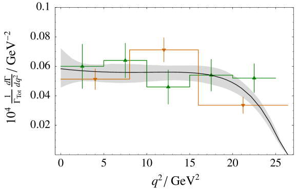
Figure 1: Differential decay rate with $68\%$ CL band (shaded) together with experimental partial branching fractions divided by the appropriate bin-width (histograms and points). Downward triangles denote combined CLEO/Belle/BaBar tagged analysis results, upward triangles BaBar untagged results.

In figure 1 we show the differential decay rate calculated using our fitted form factor and $|V_{ub}|$. Partial branching fractions calculated for the same bins as used experimentally are given in the last column of table 2. Our calculated total branching ratio turns out to be $(1.3\pm 0.08)\times 10^{-4}$, in good agreement with $(1.34\pm 0.08\pm 0.08)\times 10^{-4}$ quoted by the Heavy Flavours Averaging Group (HFAG) [37].

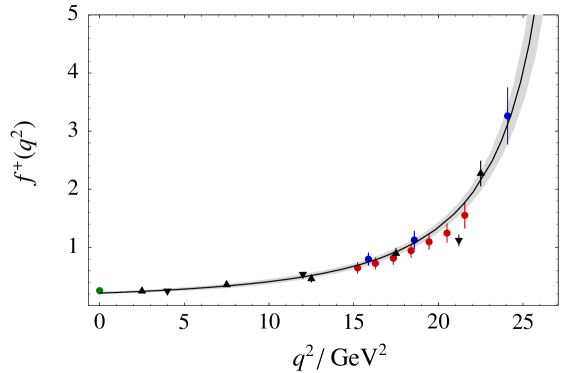
Figure 2: Form factor $f^{+}(q^{2})$ with $68\%$ CL band (shaded) together with LCSR and lattice QCD inputs (circles). Downward (CLEO/Belle/BaBar) and upward (BaBar) triangles show estimates for the form factors deduced from the experimental partial branching fractions assuming a constant $f^{+}$ over each bin and using our central fitted value of $|V_{ub}|$.

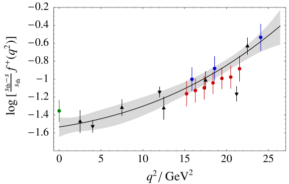
Figure 3: Same as in figure 2 but for the quantity $\log[(s_{\mathrm{th}}-s)f^{+}(q^{2})/s_{\mathrm{th}}]$.

In figure 2 we show the form factor $f^{+}$. Figure 3 shows the quantity $\log[(s_{\mathrm{th}}-s)f^{+}(q^{2})/s_{\mathrm{th}}]$ where the details of the fit and inputs can be better seen. Incorporating the experimental information still allows a fit which is perfectly consistent with the theory form factor inputs. Note that the “experimental” points (shown by triangles) in figures 2, 3 and 4 are obtained from the partial branching fractions by assuming a constant form factor over the corresponding bin and are included as a guide for convenience. The deviation from our curves of the highest $q^{2}$-bin CLEO/Belle/BaBar form factor point is not significant since the form factor varies rapidly in this region and the calculated partial branching fraction agrees within errors with the experimental one (as shown in table 2).

The inclusion of experimental shape information has balanced the tendency for the LCSR point at $q^{2}=0$ to reduce the value of $|V_{ub}|$. To illutrate this, using only the theory inputs and comparing to the total branching fraction allows the fitted form factor to pass through the LCSR point and leads to $|V_{ub}|=(3.73\pm 0.51\pm 0.16)\times 10^{-3}$, where the first error comes from the fit and the second error is from the HFAG total branching fraction quoted above. Moreover calculated partial branching fractions from this fit are above experiment at low $q^{2}$ and below it at high $q^{2}$.

We have checked that our determination of $f^{+}$ is consistent with the dispersive bound. We computed $P\phi f^{+}$ as a function of $z(q^{2},t_{0})$, where $P$, $\phi$, $z$ and $t_{0}=s_{\mathrm{th}}[1-(1-q^{2}_{\mathrm{max}}/s_{\mathrm{th}})^{1/2}]$ are defined in reference [6]. This is shown in figure 4. When $P\phi f^{+}$ is Taylor-expanded in powers of $z$, the constraint is that the sum of squares of the expansion coefficients is bounded above by $1$. We find that a cubic polynomial is an excellent fit (see figure 4) and the coefficients are,

$$a_{0}=0.026\pm 0.002,\quad a_{1}=-0.037\pm 0.021,\quad a_{2}=-0.103\pm 0.041,\quad a_{3}=0.25\pm 0.37.$$ (12)

with $\sum a_{i}^{2}=0.10^{+0.35}_{-0.06}<1$. The errors for the $a_{i}$ coefficients arise from the variation of our form factor Monte-Carlo propagated to $P\phi f^{+}$ (see the bands in figure 4).

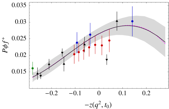
Figure 4: Same as in figure 2 but for the quantity $P\phi f^{+}$ plotted as a function of $-z(q^{2},t_{0})$. The dashed line sitting on top of the central line is a cubic polynomial fit to $P\phi f^{+}$, see text and equation (12).

One may wonder how important the inclusion of the LCSR point is for the fit. Removing this input leads to $|V_{ub}|=4.24(40)\times 10^{-3}$, $f^{+}(0)=0.166(31)$, so $|V_{ub}|$ increases by $6\%$, half its error, while the error itself increases by $15\%$. Moreover, we checked that the output percentage error in $|V_{ub}|$ would decrease about one-eighth as fast as the percentage error on the LCSR input decreases. Hence the LCSR input is important for its effect on the central value, but the overall error in $|V_{ub}|$ is not much reduced. The key to the small overall error, as noted in [5, 6, 7] is to use a model-independent functional form with enough parameter freedom to allow the data to determine the form-factor shape. The Omnès form is relatively simple and is conveniently expressed in terms of form factor inputs at a set of $q^{2}$ values.

We have not included possible statistical correlations within and between the HPQCD and FNAL lattice inputs (the lattice analysis produces statistical correlations between the form factor values at different $q^{2}$, while both simulations are based on the same gauge field ensembles, although they use different heavy-quark formalisms). We modelled correlations of the statistical errors both within and between the HPQCD and FNAL inputs by creating a statistical error matrix

$$C_{\mathrm{stat}\,ij}=r\sigma_{i}\sigma_{j}+(1-r)\sigma_{i}^{2}\delta_{ij}$$

where $r$ is a correlation coefficient and $\sigma_{i}$ are the statistical errors on the individual inputs quoted by the HPQCD and FNAL groups. We added this to the block-diagonal systematic error matrix to create the full covariance matrix. For $r=0.25$ our fit results are essentially unchanged, while for $r=0.81$, the central value of $|V_{ub}|$ moves down by one third of the original error (away from the inclusive determination) while the error itself grows by $10\%$. We conclude that these correlations should be included if they are known, but unless they are strong, they will not have a substantial effect.

On the experimental side, we have replaced the inputs used here with partial branching fraction data from BaBar in $12$ bins of $q^{2}$ [38], for which full correlation matrices are given. We find results completely consistent with those given above, but do not quote them since the data in [38] are still preliminary.

Applying soft collinear effective theory (SCET) to $B\to\pi\pi$ decays allows a factorisation result to be derived which leads to a model-independent extraction of the form factor (multiplied by $|V_{ub}|$) at $q^{2}=0$ [39]. We quote the result from our fit:

$$|V_{ub}|f^{+}(0)=(8.7\pm 1.0)\times 10^{-4}$$ (13)

to be compared to $|V_{ub}|f^{+}(0)=(7.2\pm 1.8)\times 10^{-4}$ in [39]. In view of this, we have tried replacing the LCSR input at $q^{2}=0$ with the $|V_{ub}|f^{+}(0)$ constraint from SCET. The result here, $|V_{ub}|=4.24(40)\times 10^{-3}$, $f^{+}(0)=0.167(27)$, is completely compatible with that using the lattice inputs alone ($|V_{ub}|=4.24(40)\times 10^{-3}$, $f^{+}(0)=0.166(31)$). The SCET and LCSR points are not really compatible with each other when combined separately with the lattice inputs. Not surprisingly, the effects are larger on $f^{+}(0)$ than on $|V_{ub}|$. Finally, we also tried using both LCSR and SCET inputs, for which the results ($|V_{ub}|=3.96(34)\times 10^{-3}$, $f^{+}(0)=0.210(22)$) are compatible with our quoted values above.

To conclude, we have presented a theoretically-based procedure to analyse exclusive $B\to\pi$ semileptonic decays. Starting from very general principles we propose a simple parameterization for the form factor $f^{+}$, equation (6), requiring as input only knowledge of the form factor at a set of points. We have used this to combine theoretical and experimental inputs, allowing a robust determination of $|V_{ub}|$ and of the $q^{2}$ dependence of the form factor itself. Our error for $|V_{ub}|$ is reduced compared to the current exclusive world-average value, $|V_{ub}|=(3.80\pm 0.27\pm 0.47)\times 10^{-3}$, from HFAG [37] and is competitive in precision with the inclusive world-average value, $|V_{ub}|=(4.45\pm 0.20\pm 0.26)\times 10^{-3}$ [37]. Moreover we do not find a discrepancy between our exclusive result and the inclusive world average.

Acknowledgements

We thank Iain Stewart for discussions on dispersive bounds. JMF acknowledges PPARC grant PP/D000211/1, the hospitality of the Universidad de Granada and the Institute for Nuclear Theory at the University of Washington, and thanks the Department of Energy for partial support. JN acknowledges the hospitality of the School of Physics & Astronomy at the University of Southampton, Junta de Andalucia grant FQM0225, MEC grant FIS2005–00810 and MEC financial support for movilidad de Profesores de Universidad españoles PR2006–0403.

References

- [1] CLEO Collaboration, S.B. Athar et al., Phys. Rev. D68, 072003 (2003), hep-ex/0304019.
- [2] BABAR Collaboration, B. Aubert et al., Phys. Rev. D72, 051102 (2005), hep-ex/0507003.
- [3] Belle Collaboration, T. Hokuue et al. (2006), hep-ex/0604024.
- [4] BABAR Collaboration, B. Aubert (2006), hep-ex/0607089.
- [5] M.C. Arnesen, B. Grinstein, I.Z. Rothstein, and I.W. Stewart, Phys. Rev. Lett. 95, 071802 (2005), hep-ph/0504209.
- [6] T. Becher and R.J. Hill, Phys. Lett. B633, 61 (2006), hep-ph/0509090.
- [7] R.J. Hill (2006), hep-ph/0606023.
- [8] E. Gulez et al., Phys. Rev. D73, 074502 (2006), hep-lat/0601021.
- [9] M. Okamoto, PoS LAT2005, 013 (2006), hep-lat/0510113.
- [10] Fermilab Lattice, MILC and HPQCD Collaboration, P.B. Mackenzie et al., PoS LAT2005, 207 (2006).
- [11] P. Ball and R. Zwicky, Phys. Rev. D71, 014015 (2005), hep-ph/0406232.
- [12] UKQCD Collaboration, D.R. Burford et al., Nucl. Phys. B447, 425 (1995), hep-lat/9503002.
- [13] UKQCD Collaboration, L. Del Debbio, J.M. Flynn, L. Lellouch, and J. Nieves, Phys. Lett. B416, 392 (1998), hep-lat/9708008.
- [14] S. Hashimoto, et al., Phys. Rev. D58, 014502 (1998), hep-lat/9711031.
- [15] JLQCD Collaboration, S. Aoki et al., Phys. Rev. D64, 114505 (2001), hep-lat/0106024.
- [16] UKQCD Collaboration, K.C. Bowler et al., Phys. Lett. B486, 111 (2000), hep-lat/9911011.
- [17] A. Abada et al., Nucl. Phys. B619, 565 (2001), hep-lat/0011065.
- [18] A.X. El-Khadra, et al., Phys. Rev. D64, 014502 (2001), hep-ph/0101023.
- [19] P. Ball and V.M. Braun, Phys. Rev. D58, 094016 (1998), hep-ph/9805422.
- [20] P. Ball, JHEP 09, 005 (1998), hep-ph/9802394.
- [21] A. Khodjamirian, et al., Phys. Rev. D62, 114002 (2000), hep-ph/0001297.
- [22] P. Ball and R. Zwicky, JHEP 10, 019 (2001), hep-ph/0110115.
- [23] W.Y. Wang and Y.L. Wu, Phys. Lett. B515, 57 (2001), hep-ph/0105154.
- [24] J.G. Korner, C. Liu, and C.T. Yan, Phys. Rev. D66, 076007 (2002), hep-ph/0207179.
- [25] W.Y. Wang, Y.L. Wu, and M. Zhong, Phys. Rev. D67, 014024 (2003), hep-ph/0205157.
- [26] Z.G. Wang, M.Z. Zhou, and T. Huang, Phys. Rev. D67, 094006 (2003).
- [27] D. Becirevic and A.B. Kaidalov, Phys. Lett. B478, 417 (2000), hep-ph/9904490.
- [28] L.P. Lellouch, Nucl. Phys. B479, 353 (1996), hep-ph/9509358.
- [29] M. Fukunaga and T. Onogi, Phys. Rev. D71, 034506 (2005), hep-lat/0408037.
- [30] S. Mandelstam, Phys. Rev. 112, 1344 (1958).
- [31] K.M. Watson, Phys. Rev. 95, 228 (1954).
- [32] C. Albertus, et al., Phys. Rev. D72, 033002 (2005), hep-ph/0506048.
- [33] E. Pallante and A. Pich, Nucl. Phys. B592, 294 (2001), hep-ph/0007208.
- [34] C. Bourrely, I. Caprini, and L. Micu, Eur. Phys. J. C27, 439 (2003), hep-ph/0212016.
- [35] A.D. Martin and T.D. Spearman, Elementary Particle Theory (North Holland, Amsterdam, 1970) p. 401.
- [36] J.M. Flynn and J. Nieves, Phys. Lett. B505, 82 (2001), hep-ph/0007263.
- [37] Heavy Flavor Averaging Group (HFAG) (2006), hep-ex/0603003.
- [38] BABAR Collaboration, B. Aubert et al. (2006), hep-ex/0607060.
- [39] C.W. Bauer, D. Pirjol, I.Z. Rothstein, and I.W. Stewart, Phys. Rev. D70, 054015 (2004), hep-ph/0401188.