Gravitino Dark Matter Scenarios with Massive Metastable Charged Sparticles at the LHC

Abstract:

We investigate the measurement of supersymmetric particle masses at the LHC in gravitino dark matter (GDM) scenarios where the next-to-lightest supersymmetric partner (NLSP) is the lighter scalar tau, or stau, and is stable on the scale of a detector. Such a massive metastable charged sparticle would have distinctive Time-of-Flight (ToF) and energy-loss ($dE/dx$) signatures. We summarise the documented accuracies expected to be achievable with the ATLAS detector in measurements of the stau mass and its momentum at the LHC. We then use a fast simulation of an LHC detector to demonstrate techniques for reconstructing the cascade decays of supersymmetric particles in GDM scenarios, using a parameterisation of the detector response to staus, taus and jets based on full simulation results. Supersymmetric pair-production events are selected with high redundancy and efficiency, and many valuable measurements can be made starting from stau tracks in the detector. We recalibrate the momenta of taus using transverse-momentum balance, and use kinematic cuts to select combinations of staus, taus, jets and leptons that exhibit peaks in invariant masses that correspond to various heavier sparticle species, with errors often comparable with the jet energy scale uncertainty.

1 Introduction

One of the main motivations for supersymmetry is the existence of a natural candidate for cold dark matter (CDM) [1, 2] in models in which R-parity is conserved, thus making the lightest supersymmetric partner (LSP) stable. Most detector studies of supersymmetric models have focused on the constrained minimal supersymmetric standard model (CMSSM), in which the soft supersymmetry-breaking parameters: the gaugino masses $m_{1/2}$, the scalar masses $m_{0}$ and the trilinear parameters $A_{0}$, are each assumed to be universal at some high scale, and the LSP is assumed to be the lightest neutralino. With the precision measurement of the CDM density obtained by combining data from the WMAP experiment with other cosmological data [3, 4], and taking into account accelerator constraints, the CMSSM parameter space has become quite restricted [5]. Collider signatures of these models typically involve missing energy from escaping neutralinos.

However, there is another plausible CDM candidate in R-conserving supersymmetric models, namely the supersymmetric partner of the graviton, the gravitino [6, 7, 8, 9, 10, 11, 12, 13, 14, 16, 17, 15, 18, 19]. The gravitino mass, $m_{3/2}$, is poorly constrained by accelerator experiments and the astrophysical and cosmological constraints are very different from those on the neutralino. In gravitino dark matter (GDM) scenarios the next-to-lightest supersymmetric partner (NLSP) has a very long lifetime, particularly in gravity-mediated models of supersymmetry breaking, in which the gravitino’s couplings to other particles are suppressed by an inverse power of the Planck mass. In the case of a neutralino NSLP and an arbitrary gravitino mass, the allowed parameter space of CMSSM is expanded and the classic supersymmetric signature of missing energy at colliders remains. Here we study instead the intriguing possibility of a charged NLSP, in particular the case where the NSLP is the lighter stau, $\tilde{\tau}_{1}$. In gravity-mediated models with R conservation, the stau would be stable on the scale of a detector, and every supersymmetric event would contain a pair of massive metastable charged leptons. Because of their large mass and low velocities, these would have distinctive Time-of-Flight (ToF) and energy-loss ($dE/dx$) signatures. Moreover, most supersymmetric events in such stau NLSP scenarios also contain a pair of $\tau$ leptons as well as energetic jets and possibly other leptons [20].

In Section 2 we review the properties of three benchmark points for GDM models with a stau NLSP, which were first proposed in [20]. Subsequently, in Section 3, we summarise the documented expectations for the ATLAS detector response to the metastable $\tilde{\tau}_{1}$ with limited integrated luminosity, focusing on the accuracy achievable at the LHC in measurements of the stau mass and momentum for these benchmark points, taking into account trigger information and looking at cuts to reject possible backgrounds. In Section 4 we use a parametrised fast simulation to investigate the capabilities of ATLAS to measure the masses of other supersymmetric particles in GDM models by reconstructing supersymmetric cascade decays. For this we use as building blocks the staus themselves, the accompanying $\tau$ leptons, whose full momenta we can reconstruct using transverse momentum information, hadronic jets and any accompanying charged leptons. In the benchmark scenario $\epsilon$, with a relatively light spectrum, many different sparticle species may be reconstructed in this way and their masses measured with a high accuracy. In the heavier benchmark scenarios $\zeta,\eta$, fewer sparticles can be reconstructed and with worse accuracy, even at the fairly high integrated luminosity considered. Finally, in Section 5 we draw our main conclusions.

2 The GDM Benchmark Points

Three GDM benchmark points with a $\tilde{\tau}_{1}$ NLSP, named $(\epsilon,\zeta,\eta)$, were proposed in [20]. These were formulated in the framework of minimal supergravity (mSUGRA) models [21], in which the gravitino mass is fixed equal to the universal soft supersymmetry-breaking masses of scalar particles at a GUT input scale: $m_{3/2}=m_{0}$, and there is a simple relation between the soft trilinear and bilinear parameters: $A_{0}=B_{0}+m_{0}$. This relationship can be used to fix the ratio of the Higgs vacuum expectation values $\tan\beta$ from the electroweak vacuum conditions. Further, the value $A_{0}=(3-\sqrt{3})\,m_{0}$ found in the Polonyi model of supersymmetry breaking in a hidden sector is assumed [22]. The resulting allowed GDM parameter space may be displayed as a region in the $(m_{1/2},m_{0})$ plane, subject to theoretical, phenomenological and cosmological constraints.

This region is restricted, in particular, by the requirement of maintaining the cosmological concordance between the values of the baryon-to-entropy ratio inferred from the cosmic microwave background radiation and from astrophysical light-element abundances, which constrain NLSP decays and cut the parameter space down to a wedge in the $(m_{1/2},m_{0})$ plane, throughout which the $\tilde{\tau}_{1}$ is the NLSP and is metastable. The shape of this wedge, taken from [20], is shown in Fig. 1 as the area restricted to lie below the upper black line. The $\epsilon$ benchmark point is a collider-friendly point at low values of $m_{1/2}$ and $m_{0}$ sitting near the apex of the cosmologically-allowed wedge. It features relatively large production cross sections for supersymmetric events at the LHC, as seen in Table 1. The $\zeta$ and $\eta$ points represent more challenging scenarios at higher values of $m_{1/2}$, and hence with lower cross sections. The point $\zeta$ lies at the boundary of the cosmologically-allowed area, where the NLSP lifetime exceeds $10^{6}$ s, whereas $\eta$ is characteristic of models with a relatively low $\tilde{\tau}_{1}$ lifetime $\sim 10^{4}$ s, shown as the lower black line in Fig. 1, below which additional constraints due to hadronic interactions in the early universe become important [25, 26, 27]. A recent analysis indicates that earlier constraints were overly restrictive, so that the point $\eta$ lies well within the allowed region [23]. None of these three benchmark points give the full amount of CDM required by WMAP, if one takes into account only the gravitino abundance due to decays of the NLSP after freeze-out. The missing CDM could be provided by additional gravitino production mechanisms in the early Universe, or other components of CDM such as axions.

Model	$\sigma(\tilde{\tau}_{1}\tilde{\tau}_{1}^{*})$	$\sigma(\tilde{g}\tilde{g})$	$\sigma(\tilde{g}\tilde{q})$	$\sigma(\tilde{q}\tilde{q})$	$\sigma(\tilde{q}\tilde{q}^{*})$	$\sigma(\tilde{\chi}^{0}_{2}\tilde{\chi}^{\pm}_{1})$
$\epsilon$	$0.0242$	$0.220$	$1.36$	$0.755$	$0.445$	$0.114$
$\zeta$	$0.00124$	$0.000194$	$0.00391$	$0.00851$	$0.00148$	$0.00229$
$\eta$	$0.00157$	$0.000195$	$0.00394$	$0.00859$	$0.00150$	$0.00229$

Table 1: The main supersymmetric production cross sections at the LHC, in pb, including Drell-Yan production of $\tilde{\tau}_{1}$ pairs, pair production of strongly-interacting sparticles and associated production of neutralinos and charginos, computed to NLO for the GDM benchmarks using Prospino2 [24]. Note that these differ from those given in [20], mainly because of the larger gluino and squark masses obtained from ISAJET (see below) and partly because we use different parton density functions (see Section 3).

For the purposes of this paper, the effective masses of sparticles at the electroweak scale for these benchmark points were calculated by running the universal high-scale masses down to low scales using ISAJET 7.69 [28]. This gives somewhat larger masses than found in [20] using the SSARD code, in particular for the strongly-interacting sparticles. Both the GUT-scale input parameters and the resulting physical masses are given in Table 2 (as in [20], we assume sign$(\mu)=+$ and $m_{t}=178$ GeV for all three points). The decay widths and branching ratios of the supersymmetric particles were re-calculated from these masses using the decay code SDECAY 1.1a [29], except for the three-body decays of the first- and second-generation right-handed sleptons, which are not included in SDECAY, and whose decays instead are taken from ISAJET.

Model	$\epsilon$	$\zeta$	$\eta$
$m_{1/2}$	440	1000	1000
$m_{0}$	20	100	20
$\tan{\beta}$	15	21.5	23.7
$A_{0}$	-25	-127	-25
Masses
$|\mu|$	569	1186	1171
h0	119	124	124
H0	626	1293	1261
A0	622	1285	1253
H±	632	1296	1264
$\chi^{0}_{1}$	175	417	417
$\chi^{0}_{2}$	339	805	804
$\chi^{0}_{3}$	574	1192	1176
$\chi^{0}_{4}$	587	1200	1184
$\chi^{\pm}_{1}$	340	807	806
$\chi^{\pm}_{2}$	587	1200	1184
$\tilde{g}$	1026	2191	2191
$e_{L}$, $\mu_{L}$	306	684	677
$e_{R}$, $\mu_{R}$	171	387	374
$\nu_{e}$, $\nu_{\mu}$	290	669	662
$\tau_{1}$	153	338	319
$\tau_{2}$	309	677	670
$\nu_{\tau}$	288	660	653
$u_{L}$, $c_{L}$	935	1991	1988
$u_{R}$, $c_{R}$	902	1911	1908
$d_{L}$, $s_{L}$	938	1993	1990
$d_{R}$, $s_{R}$	899	1903	1900
$t_{1}$	710	1545	1553
$t_{2}$	900	1842	1840
$b_{1}$	852	1807	1804
$b_{2}$	883	1851	1846

Table 2: Proposed GDM benchmark points taken from [20]. Mass spectra [GeV] are calculated using ISAJET 7.69 [28].

One of the most important decays of these GDM models, at least for those within the reach of the LHC, is that of the right-handed squark: $\tilde{q}_{R}\to q\tilde{\chi}_{1}^{0}$ with branching ratios of almost 100% at all three points. This is followed by the decay $\tilde{\chi}_{1}^{0}\to\tau\tilde{\tau}_{1}$ in a large fraction of events (92/75/69 % for the three points), so that the decays of two right-handed squarks result in the relatively clean final states $qq\tau\tau\tilde{\tau}_{1}\tilde{\tau}_{1}$ in a large fraction of the events. From the branching ratio of this decay chain shown in the left plot of Fig. 1, we see that this signature is a quite generic feature for the class of GDM models with a $\tilde{\tau}$ NLSP. In the experiments it should be possible to trigger on the pair of high-$p_{T}$ jets produced in the primary $\tilde{q}_{R}\to q\tilde{\chi}_{1}^{0}$ or the pair of tau jets, and one can then identify the stau by its peculiar signature as a slow moving muon and measure its mass and momentum to high precision, as discussed in the next Section. One can also identify the decay products of the $\tau$ and reconstruct the full $\tau$ momenta using transverse momentum balance, as we show in Section 4. Thus, these events can be fully reconstructed and we can make a precise determination of the masses of all three supersymmetric particles involved in the decay cascade. From this decay chain one may also be able think of reconstructing the gluino $\tilde{g}$ from its decays into squark-quark pairs, as we discuss later for benchmark point $\epsilon$.

Figure 1: Total branching ratios for the $\tilde{q}_{R}\to q\tilde{\chi}_{1}^{0}\to q\tau\tilde{\tau}_{1}$ (left) and $\tilde{q}_{L}\to q\tilde{\chi}_{2}^{0}\to q\ell\tilde{\ell}_{L}\to q\ell\ell\tilde{\chi}_{1}^{0}\to q\ell\ell\tau\tilde{\tau}_{1}$ (right) decay chains in the $(m_{1/2},m_{0})$ parameter plane. The solid black lines indicate the boundary of the cosmologically allowed region of parameter space explored in [20].

Figure 2: Branching ratio for the decay chains $\tilde{\chi}_{1}^{\pm}\to\tau\tilde{\nu}_{\tau}\to\tau W\tilde{\tau}_{1}$ (left) and $\tilde{\chi}_{1}^{0}\to\ell\tilde{\ell}_{R}\to\ell\ell\tau\tilde{\tau}_{1}$ (right) in the $(m_{1/2},m_{0})$ parameter plane. The solid black lines indicate the cosmologically allowed region of parameter space explored in [20].

The decays of left-handed squarks have in general more leptons in the final state, for example when decaying via $\tilde{\chi}_{2}^{0}\to\ell\tilde{\ell}_{L}$ and $\tilde{\ell}_{L}\to\ell\tilde{\chi}_{1}^{0}$, with the total branching ratio shown in the right plot of Fig. 1. With knowledge of the $\tilde{\chi}_{1}^{0}$ mass, this makes possible the reconstruction of the left-handed slepton and the $\tilde{\chi}_{2}^{0}$. However, left-handed squark decays into charginos are more difficult to use because of neutrinos in the final state, either directly from the chargino decay, or from the leptonic decay of a $W$.

Whilst the branching ratio of the left-handed squark is too low to search for events with two such decay chains, the considerations for triggering, particle identification and reconstruction are similar to those for the right-handed squark. The appearance of hard leptons help identify the decay chain, but give additional combinatorial difficulties in particle identification as we will see in Section 4. Nevertheless, it seems possible to reconstruct this decay chain, at least for the benchmark point $\epsilon$, as we discuss later.

At the $\epsilon$ benchmark point the supersymmetric events are dominated by gluino/squark production followed by cascade decays. For the low cross-section benchmark points $\zeta$ and $\eta$, we see from Table 1 that these events make up a smaller fraction of the total number of supersymmetric events. Here Drell-Yan and associated neutralino and chargino production become more important. These events feature less jet activity and heavier, slower staus, and may lead to some trigger problems (see Section 3.2). By considering only the Drell-Yan cross-section, taking into consideration triggering and reconstruction efficiencies for stau pair production, one could investigate the reach of the LHC in setting model-independent exclusion limits on the mass of the stau. However, this would require a very detailed understanding of the effects of the background cuts suggested in Section 3.3 on SM events in the limit where the background tends to zero, and is perhaps best left to a full detector simulation. Here we will instead focus on some interesting decay chains starting from the associated production. The branching ratio of the decay $\tilde{\chi}_{1}^{\pm}\to\tau\tilde{\nu}_{\tau}\to\tau W\tilde{\tau}_{1}$ is shown in Fig. 2, and is almost identical to that for the decay $\tilde{\chi}_{2}^{0}\to\nu_{\tau}\tilde{\nu}_{\tau}\to\nu_{\tau}W\tilde{\tau}_{1}$, as the decays differ essentially only by the mass of the tau. If we can reconstruct the $W$ produced in both cases from its hadronic decay and combine with the correct stau candidate, this gives us direct access to the tau-sneutrino and, possibly, chargino masses.

Among the lighter particles of Table 2 that one would expect to be copiously produced at the LHC in the case the $\epsilon$ benchmark, we have not yet discussed decays involving the $\tilde{\ell}_{R}$, the right-handed selectron or smuon. These are dominantly produced in decays of neutralinos, the only exception being the direct pair-production of the sleptons, which have low cross sections. In fact, only in the decay of the lightest neutralino is there a significant rate, due to the preference for decays to left-handed sleptons, and even here it is suppressed relative to decays to the lighter stau. The $\tilde{\ell}_{R}$ decays in turn almost exclusively to the three bodies $\ell\tau\tilde{\tau}_{1}$. In the right plot of Fig. 2 we show the total branching ratio of the decay $\tilde{\chi}_{1}^{0}\to\ell\tilde{\ell}_{R}\to\ell\ell\tau\tilde{\tau}_{1}$. One could hope to reconstruct the $\tilde{\ell}_{R}$ mass from this decay, starting from the stau. However, the low branching ratio at the point $\epsilon$, combined with the soft spectra of the leptons from the decay, due to the small mass differences, makes this very difficult. Our attempts leave us with only a few events. The larger branching ratios and harder leptons of the two other benchmarks are unfortunately balanced out by the overall much lower cross sections. It thus seems to be very challenging to reconstruct the $\tilde{\ell}_{R}$ in GDM models at the LHC, and we do not discuss the $\tilde{\ell}_{R}$ further.

The first four decay chains we discussed above will be the main focus of our attempts at reconstructing supersymmetric masses in Section 4. The fact that, as shown in Figs. 1 and 2, the total branching ratios for these decay chains are relatively high across large regions of the $(m_{1/2},m_{0})$ plane, with a dominating branching ratio for the chain initiated by $\tilde{q}_{R}\to q\tilde{\chi}_{1}^{0}$ in all the explored range of the allowed parameter space, up to values of $m_{1/2}\sim 2$ TeV, suggests that the techniques discussed here would be of wide utility at the LHC.

For the most part, we limit our discussions to simulations of the high-cross-section benchmark point $\epsilon$, and only summarise our results for the other two points. We draw attention to instances where there are important differences between the benchmark points, and we refer the reader to [20] for further details about them.

3 Fast Monte Carlo Simulation

For the fast simulation we have generated proton-proton collisions at the LHC energy using PYTHIA 6.326 [30] and CTEQ 5M1 parton distribution functions [31]. For the $\epsilon$ benchmark point we show results on mass measurements for a total integrated luminosity of $30~{}\text{fb}^{-1}$, corresponding to the planned initial running of the LHC at low luminosity. In the cases of the $\zeta$ and $\eta$ points, which have relatively low cross sections, we show results for statistics equivalent to $300~{}\text{fb}^{-1}$. These may then be viewed as estimates of the ultimate precisions achievable for these benchmark points without an upgrade of the LHC luminosity.

3.1 Parametrisation of Detector

The detector simulation has been carried out using the generic LHC detector simulation AcerDET 1.0 [32], taking the ATLAS detector as our model for a LHC detector. Here we give a short summary of the most important choices made for the AcerDET settings: We consider a lepton to be identified if it has transverse momentum $p_{T}>5(6)$ GeV and $|\eta|<2.5$ for electrons (muons). A lepton is considered isolated if it is at a distance $\Delta R>0.4$, where $\Delta R\equiv\sqrt{(\Delta\phi)^{2}+(\Delta\eta)^{2}}$, from other leptons and jets, and if the transverse energy deposited in a cone $\Delta R=0.2$ around the lepton is less than $10$ GeV. Jets are reconstructed by a cone-based algorithm from clusters and are accepted if the jet has $p_{T}>15$ GeV within a cone $\Delta R=0.4$. The jets are re-calibrated using an included flavour-independent parametrisation, optimised to give the correct resonance mass in dijet decays. We use the $p_{T}$ parametrised $b$-tagging efficiency and light jet rejection, for a low-luminosity environment, given in [33]. For tau jets we use a lower cut on transverse momentum of $p_{T}>20$ GeV, and the parametrised tau-tagging efficiency and rejection factors from [34].

For the detector’s response to staus, we take our parametrisation of the momentum resolution from [35, 36], which performed a full simulation of the response of the ATLAS muon system to a metastable stau of mass $101$ GeV, in a Gauge Mediated Supersymmetry Breaking (GMSB) model. This momentum dependent resolution is used to smear the stau momentum in the detector simulation. We have performed a smearing with width $\sigma_{p}$, given by

$$\frac{\sigma_{p}}{p}=k_{1}p\oplus k_{2}\sqrt{1+\frac{m_{\tilde{\tau}_{1}}^{2}}{p^{2}}}\oplus\frac{k_{3}}{p},$$ (1)

where $k_{1}$ is the parameter of the sagitta measurement error, $k_{2}$ represents the multiple scattering and $k_{3}$ the fluctuation of energy loss in the calorimeter. From [35] we take the values $k_{1}=0.0118$, $k_{2}=0.02$ and $k_{3}=89$.

For the measurement of the velocity of staus and muons, we use the parametrisation of the velocity resolution from [35, 36]. In our simulation we smear the true velocity by:

$$\frac{\sigma_{\beta}}{\beta}=0.028\,\beta,$$ (2)

which was found by looking at the fit quality of tracks in the muon system as a function of the particle’s assumed arrival time in the Monitored Drift Tubes (MDT), subsequently minimising the $\chi^{2}$ as a function of the arrival time to find the correct Time-of-Flight (ToF). This is a conservative estimate of the resolution as the simulation was carried out in the central detector, for $\eta=0.1$. For larger pseudo-rapidities the resolution is expected to improve, due to a longer flight path. An alternative way to measure the ToF would be to use the timing of hits in the Resistive Plate Chambers (RPC), responsible for muon triggering, which may be able to provide similar precision.

3.2 Trigger

It was suggested in [20] that the triggering efficiency for events in GDM scenarios will be high. A full simulation of these benchmark points, which will include triggers, is under way [37], and we have every reason to believe that due to the generically large jet and lepton activity in the supersymmetric events we will have trigger efficiencies in the high $90$% range for all three benchmarks. As an estimate of the trigger, in our fast simulation we have required each event to have at least one of the following:

• A jet with $p_{T}>290$ GeV,

• three jets with $p_{T}>130$ GeV,

• four jets with $p_{T}>90$ GeV,

• one muon or stau with $p_{T}>20$ GeV, or

• two muons or staus with $p_{T}>6$ GeV.

These are the jet and muon trigger thresholds for the ATLAS detector, taken from [38], where we conservatively use the high-luminosity thresholds and ignore electromagnetic, missing-energy and tau triggers. Since one may fail to trigger on a slow stau in the normal running of the LHC detectors because it arrives at the trigger station too late, we additionally require triggering staus to have a velocity of $\beta\gamma>0.9$. This number is a conservative estimate from the ATLAS geometry, to give a trigger in the correct bunch crossing. Staus with $|\eta|\approx 1$ have the longest distance to travel between RPC layers. Given a $25$ ns gap between bunch crossings and a distance of $\approx 15.5$ m to the outer RPC layer the critical velocity is $\beta=0.67$, or $\beta\gamma=0.9$, ignoring any significant energy loss.

3.3 Background

In order to separate the staus from background muons in the supersymmetric events, and to remove the Standard Model background, we use the following cuts, which we will refer to as the standard GDM cuts:

• There should be exactly two stau candidates in each event,

• these should be isolated and within the geometrical acceptance of the muon chambers as per the requirements for the muons listed above,

• they should have $p_{T}>50$ GeV,

• they should have a velocity $\beta\gamma<6.0$, and

• they should have a mass estimate from their momentum and velocity that is consistent with the stau mass after it has been measured (see Section 4.1);

• in addition, the sum of the number of leptons (muons or electrons) with $p_{T}>10$ GeV and tau-tagged jets with $p_{T}>20$ GeV in each event should be exactly two.

The final cut is made on the basis that in GDM scenarios with a $\tilde{\tau}_{1}$ NLSP, the vast majority of events will contain two taus in addition to the pair of staus, and these should be identified to fully reconstruct the particles in the supersymmetric decay chains (see Section 4.2). Note that we have a much looser cut on $\beta\gamma$ than used in [36]. We still expect to remove most SM background because of the requirement of two stau candidates in each event, and in particular because of the extra requirement of two tau candidates.

After our trigger requirements and these cuts, we should have a very powerful rejection on Standard Model background events. We have tested this hypothesis in a fast simulation of a background sample consisting of the equivalent of $30~{}\text{fb}^{-1}$ of $t\bar{t}$ events with an NLO cross section of $737$ pb [39], and samples of $p_{T}$ binned QCD, $W$+jets, $Z$+jets and $WW/WZ/ZZ$ production events. The total numbers of events are $1.75\cdot 10^{6}$ for QCD and $2.5\cdot 10^{5}$ for the other processes. We find no events that survive the cuts listed above, and, in order to find the first events that pass the cuts, we would need to relax the velocity cut to $\beta\gamma<8.3$, after which we find one $WW/WZ/ZZ$ event that passes. However, with the limited statistics available, in particular for QCD, this null result must be interpreted with care. For example, the parametrisation of the $\beta$ resolution assumes a Gaussian shape. If the true distribution has significantly larger tails, this will affect the power of the cut on $\beta\gamma$. A full simulation study of the muon velocity resolution would be required to investigate this possibility. It is partially because of this issue that we prefer to use a loose cut on $\beta\gamma$. Despite these problems, with the additional cuts made in the searches for various supersymmetric particles presented in Section 4, we expect that the cuts presented here will render negligible the Standard Model background in our analysis.

4 Reconstruction of Masses in GDM Models

In this Section, we incorporate the parametrisation of the response of the ATLAS detector to the slow-moving $\tilde{\tau}_{1}$s from Section 3 in a fast simulation of sparticle pair production and cascade decays at an LHC detector. This enables us to assess the possibility of identifying various heavier sparticles and the precision obtainable in mass measurements in GDM models. Since we have no escaping LSP in these GDM models, we are not limited to the standard measurements of the endpoints and shapes of kinematic distributions, see e.g. [40, 41, 42, 43, 44, 45, 46, 47], and we can fully reconstruct sparticles, starting from the stau NLSP.

We begin in Section 4.1 by looking at the starting point of all our mass measurements, the measurement of the stau mass. Then, in Section 4.2 we demonstrate the complete reconstruction of the tau momenta for events with only two taus and no hard neutrinos. Section 4.3 deals with the reconstruction of the decay chain $\tilde{q}_{R}\to q\tilde{\chi}_{1}^{0}\to q\tau\tilde{\tau}_{1}$, and Section 4.4 deals with the reconstruction of the cascade $\tilde{q}_{L}\to q\tilde{\chi}_{2}^{0}\to q\ell\tilde{\ell}\to q\ell\ell\tilde{\chi}_{1}^{0}\to q\ell\ell\tau\tilde{\tau}_{1}$. Finally, in Section 4.5 we discuss the possibility of measuring sneutrino and chargino masses using dijet decays of $W$ bosons produced in supersymmetric cascade decays.

4.1 Measuring the Stau Mass

We first present an estimate of the achievable precision on the measurement of the stau mass for the parametrisation of the momentum and velocity resolution given in Section 3.1. After the trigger simulation presented in Section 3.2, and making the standard GDM cuts of Section 3.3 with the exception of the cut on the stau mass and the requirement of two tau candidates, we plot in Fig. 3 (left) a scatter plot of the measured velocity $\beta\gamma_{\rm{meas}}$ versus the measured mass for single staus, as inferred from

$$m_{\tilde{\tau}_{1}}=\frac{p_{\rm{meas}}}{\beta\gamma_{\rm{meas}}}.$$ (3)

Figure 3: Scatter plot of measured velocity $\beta\gamma_{\rm{meas}}$ versus measured mass (left), with supersymmetric events in black and SM background events in red, and a corresponding plot of the measured stau mass (right) with an additional cut on the velocity of $0.3<\beta\gamma<0.6$.

We see a large spread in the masses for high $\beta\gamma$, corresponding to high momenta. This is expected as the assumed momentum resolution deteriorates significantly above a few hundred GeV, and the velocity resolution worsens at higher velocity due to the shorter ToF. One effect of the momentum dependence of the resolution is that the spread has a clear bias towards higher masses, which would be a systematic effect for a mass measurement using all events passing the cuts. We also see a grouping of events at high $\beta\gamma$ and low masses. These are mis-measured muons that have been assigned velocities that are too low, and thus passed the GDM cuts used. This is particularly clear for the SM background events which are shown in red.

Because the low-velocity events have a much smaller spread and less bias towards higher masses, it would be advantageous to use only these in a mass measurement. As we commented in Section 3.2, the staus from these events will be missed by the trigger system because they are too slow. This does not mean that they would be missed completely by the LHC detectors, since their muon systems are designed sufficiently robustly as to record hits in a large time window after a collision. However, it does mean that we will have to rely on other triggers, e.g., calorimetric triggers, or triggers on muons from the decay of the heavier sparticles. Exactly how far down in velocity it is possible to go must be the subject of full detector studies that lie beyond the scope of this paper. In [35] the velocities of the staus were found to be measurable at least down to $\beta\gamma=0.44$, albeit for a simulation of single staus in the muon system only. However, in [36] a conservative approach to the trigger issue was followed, ignoring events where the staus did not reach the muon chambers inside the time window of the muon triggers, and using a lower cut of $\beta\gamma\geq 0.75$. Assuming that the trigger rates from our simplified trigger cuts are not entirely unrealistic and that we can reconstruct staus with velocities down to $\beta\gamma\approx 0.3$, we make an additional cut on $\beta\gamma<0.6$ for the sample used to measure the stau mass, and plot the corresponding mass distribution in Fig. 3 (right). Fitting the mass distribution with a Gaussian we get a stau mass for the $\epsilon$ benchmark of

$$m_{\tilde{\tau}_{1}}\;=\;152.485\pm 0.021~{}{\rm GeV,}$$ (4)

to be compared with the nominal value of $m_{\tilde{\tau}_{1}}=152.475$ GeV.

To investigate the dependence of the measured stau mass on the lower limit on the velocity of staus that we can identify, we show in Fig. 4 the reconstructed stau mass as a function of the lower $\beta\gamma$ cut value for three different values of the upper cut on $\beta\gamma$. The general tendency is, as could be expected, an increase in the systematic error, represented by the increase in distance from the nominal mass value, as the lower cut value is raised and low-velocity events are discarded . As the lower cut approaches the upper cut value, this effect flattens out, while of course the statistical error increases with the reduction in the number of events. It is clear that, for a lower cut on $\beta\gamma$, in choosing the upper cut one must trade the loss of statistics against the reduction of systematic error from the higher-velocity staus. We see that there is very little change in the stau mass determination if the lower limit on $\beta\gamma$ is increased to 0.44 [35]. We also note that the error in $m_{\tilde{\tau}}$ remains below the per-mille level even if we restrict the analysis to $0.6<\beta\gamma<0.9$. In all the examples shown in Fig. 4, the error in calculating $m_{\tilde{\tau}}$ is negligible compared with the errors encountered in the reconstruction of higher-mass states decaying into staus.

Figure 4: The stau mass from a Gaussian fit as a function of a lower cut on $\beta\gamma$. The solid circles show the results for an upper cut of $\beta\gamma<0.6$, the triangles $\beta\gamma<0.9$ and the squares $\beta\gamma<1.2$. The red line shows the nominal mass value.

Based on the clear separation of muons and staus in the scatter plot of Fig. 3, we require in the further analyses that stau candidates have inferred masses above $100$ GeV. This value was also used in the background analysis of Section 3.3. We use the stau mass of (4) in the following discussions, although the much larger errors involved in the reconstruction of heavier sparticles means that we are insensitive to the exact value, within the errors discussed in this Section. The results for the other two benchmarks are analogous, and the resulting masses can be found in Table 3. The statistical errors are at the sub-permille level, which is below the expected uncertainty on the lepton energy scale of order $0.1$%, and on the same level as the results given for various GMSB scenarios in [36]. From Fig. 4, we conclude that it should be possible also to keep the systematic error from the momentum and velocity measurements at the same level if we are able to reconstruct staus with velocities down to $\beta\gamma=0.6$.

The possibility of making further measurements on the staus by looking for staus trapped in the LHC detectors or in surrounding matter was discussed in [20]. Trapped, decaying staus could make a measurement of the stau lifetime possible, leading to an indirect determination of the gravitino mass, assuming the macroscopically determined value of the Planck scale, and could potentially even lead to a microscopic determination of the Planck scale and a test of supergravity if the gravitino mass could be measured directly from the decay kinematics [45, 48]. However, these exciting possibilities lie somewhat outside of the scope of this paper.

Model	$\epsilon$	$\zeta$	$\eta$
Mass
$\tilde{\tau}_{1}$	$152.485\pm 0.021$	$338.24\pm 0.09$	$319.02\pm 0.09$
$\tilde{\nu}_{\tau}$	$291.8\pm 1.2$	$666.4\pm 1.9$	$659.6\pm 1.1$
$\tilde{\ell}_{L}$	$307.9\pm 2.0$	$674.6\pm 3.4$	$673.5\pm 3.5$
$\tilde{\chi}^{0}_{1}$	$176.6\pm 0.9$	$418.3\pm 1.8$	$419.6\pm 3.7$
$\tilde{\chi}^{0}_{2}$	$339.2\pm 2.0$	$(796.5\pm 6.5)$	$(801.0\pm 7.2)$
$\tilde{q}_{L}$	$923.4\pm 3.7$	-	-
$\tilde{q}_{R}$	$895.8\pm 2.8$	$1811.2\pm 332.3$	-
$\tilde{b}$	$888.9\pm 57.7$	-	-

Table 3: The mass measurements and statistical errors [in GeV] obtained in the simulations of the GDM benchmark points. The numbers in brackets ( ) are obtained from a fit to the edge in the dilepton spectrum. Jet and lepton energy scale errors are not included.

4.2 Recalibrating Taus

Figure 5: Schematic drawing of the $\tau$ decay products $\vec{p}_{j_{1}}$ and $\vec{p}_{j_{2}}$, the missing momentum $\not\!\!\vec{p}_{T}$ and the reconstructed neutrino momenta $\vec{p}_{\nu_{1}}$ and $\vec{p}_{\nu_{2}}$, projected on the transverse plane.

As was already mentioned in Section 3.3, in all R-parity conserving GDM scenarios with a $\tilde{\tau}_{1}$ NLSP, with the exception of Drell-Yan pair productions of staus and some events yielding tau neutrinos, each event will contain two $\tau$s in addition to the pair of $\tilde{\tau}_{1}$s. In Section 4.1 we discussed the measurement of the $\tilde{\tau}_{1}$ mass. We can detect and measure the masses of many of the heavier sparticles by reconstructing decay chains that lead to the $\tilde{\tau}_{1}$s. For example, at benchmark point $\epsilon$, essentially $100$% of the lightest neutralinos ${\tilde{\chi}_{1}^{0}}$ decay into $\tilde{\tau}_{1}+\tau$, and this branching ratio is also very large at the other two points ($\sim 70$%). One can reconstruct a ${\tilde{\chi}_{1}^{0}}$ mass peak by combining $\tilde{\tau}_{1}$-$\tau$ pairs, but to do this one needs to know the momenta of the accompanying $\tau$s, which in turn decay and lose momentum to escaping neutrinos.

Assuming that a $\tau$ is relativistic in the laboratory frame, as will indeed be the case for any $\tau$ that would pass our acceptance criteria, its hadronic decay will give a jet and a neutrino travelling in essentially the same direction. If there are exactly two $\tau$s in an event, and no other source of missing momentum, the sum of the missing transverse momenta from the neutrinos can be projected onto the two axes formed by the hadronic tau-decay jets in the transverse plane, as illustrated in Fig. 5. Knowing the azimuthal angles of the two $\tau$s, one can determine the two components of each of the tau neutrino momenta in the transverse plane, and their momenta in the $z$ direction follow from requiring that the neutrinos travel in the same direction as the jet. The same recalibration procedure can be used for $\tau$ pair decays into one or two leptons, with leptons taking the roles of the hadronic jets, and the sum of two $\tau$ decay neutrino momenta taking the role of the single $\tau$ decay neutrino of the hadronic case.

In our tau recalibration we assume that there are no other large contributions to the missing momentum. Possible sources is the mis-measurement of jet energies or hard neutrinos from the decay of heavy particles. These will change the direction and magnitude of the missing momentum vector in the transverse plane. This can partially be checked for by testing that the direction of the missing momentum lies inside the opening angle of the two taus.

Figure 6: The relative error between the parton-level and measured momenta of $\tau$s at the $\epsilon$ (red), $\zeta$ (green) and $\eta$ (blue) benchmark points. We show the momenta both before (dotted line) and after (solid line) recalibration.

The result of this momentum recalibration is shown in Fig. 6, where we plot the relative error on the tau momentum before (dotted line) and after (solid line) recalibration, for the three benchmark points. We have used a $50$% tau-jet tagging efficiency, and require that for each event the sum of the number of tagged tau jets and leptons (no staus) with $p_{T}>10$ GeV is exactly two, to have an unambiguous pair of tau candidates for the recalibration. No trigger or background cuts have been used.

We observe a dramatic improvement in the momentum resolution compared to uncalibrated taus for all three benchmark points, although with a significant tail of taus with momenta that are too high. The smearing of the tau momentum is partially due to other contributions to the momentum imbalance as already mentioned above, leading to a mis-calibration, but also due to the mis-tagging of tau jets and/or mis-identification of leptons as coming from tau decays. These mis-identifications can also be seen in the pre-recalibration distribution, as a tail to momenta higher than the parton momentum. We see a marked difference between the $\epsilon$ benchmark and the other two, the $\epsilon$ benchmark having a worse resolution. This could be expected from the relatively lower amount of activity in $\zeta$ and $\eta$ events, where the Drell-Yan and associated production is more pervasive, resulting in fewer mis-identifications.

4.3 Reconstructing the Decay $\tilde{q}\to q\tilde{\chi}_{1}^{0}\to q\tau\tilde{\tau}_{1}$

The great majority of right-handed squark, $\tilde{q}_{R}$, decays (92 %) and a few of the left-handed squark, $\tilde{q}_{L}$, decays (4 %) at the $\epsilon$ benchmark point lead directly to the final state $q\tilde{\chi}_{1}^{0}$. To reconstruct the masses of the lightest neutralino $\tilde{\chi}_{1}^{0}$ and the first two, almost degenerate, generations of squarks, we seek to isolate events with two squarks, where both decay according to this clean decay chain 

$$\tilde{q}\to q\tilde{\chi}_{1}^{0}\to q\tau\tilde{\tau}_{1}.$$ (5)

We first select events that survive our trigger requirements and the standard GDM cuts of Section 3.3. These remove the Standard Model background, and leave us with an identified pair of staus. The energies of these staus are then re-calibrated to reflect the mass measured in Section 4.1. Using the parametrised tau-tagging described in [34], with an assumed tau-tagging efficiency of $50$%, we select events where the sum of the number of tau jets with $p_{T}>20$ GeV and leptons with $p_{T}>10$ GeV is exactly two. These are then our basis for reconstructing two taus with the technique discussed in Section 4.2. The staus and taus are matched according to charge, keeping only those events where there is an unambiguous assignment. This implies that all events with same-sign staus and all events with two tau jets are rejected. We do not consider any measurement of tau charge from the hadronic jet, leaving this as a possible improvement. However, one should note that, while this will certainly increase the available statistics, the lower tagging efficiency for hadronic tau decays compared to the efficiency of identifying leptons means that one would have roughly the same number of leptonic and hadronic tau candidates. Moreover, the momenta of the hadronic jets would be known with worse accuracy than those of the leptons.

Calculating the invariant masses of the $\tilde{\tau}$-$\tau$ combinations surviving these cuts we arrive at the distribution shown in the left plot of Fig. 7 for the $\epsilon$ benchmark. In blue we show the distribution due to events with two ${\tilde{\chi}_{1}^{0}}\to\tilde{\tau}_{1}+\tau$ decays, while the red distribution is the supersymmetric background. The total distribution shows a clear peak corresponding to the $\tilde{\chi}_{1}^{0}$ mass. We fit the distribution by a third-degree polynomial assumption for the background and a Breit-Wigner distribution for the peak, giving a $\tilde{\chi}_{1}^{0}$ mass and statistical error of

$$m_{\tilde{\chi}_{1}^{0}}\;=\;176.6\pm 0.9~{}{\rm GeV,}$$ (6)

which is to be compared with the nominal value of $m_{\tilde{\chi}_{1}^{0}}=175.2$ GeV. The wide shape of the signal distribution is due to smearing from the momentum resolution of the staus, and contributes to the overestimate of the $\tilde{\chi}_{1}^{0}$ mass. For the $\zeta$ and $\eta$ points the results are very similar, but with significantly lower statistics, even at $300~{}\text{fb}^{-1}$. The masses and errors found are listed in Table 3.

Figure 7: The $\tilde{\tau}$-$\tau$ (left) and jet-$\tilde{\tau}$-$\tau$ (right) invariant mass distributions for the $\epsilon$ benchmark point. For the left plot the blue distribution is for events containing two decays $\tilde{\chi}_{1}^{0}\to\tau\tilde{\tau}_{1}$, for the right plot events containing two $\tilde{q}\to q\tilde{\chi}_{1}^{0}\to q\tau\tilde{\tau}_{1}$ decay chains. The red distributions include all other events surviving the cuts described in the text.

To find the (right-handed) squark mass, we want to isolate events that contain two of the decays of Eq. (5). This is done by adding to the cuts used above the following:

• We require two jets with $p_{T}>300,150$ GeV,

• no other jets with $p_{T}>150$ GeV,

• missing transverse energy $E_{T}<50$ GeV, and

• to increase statistics we relax the unambiguous assignment requirement for the $\tau$-$\tilde{\tau}$ pairs, keeping those not directly excluded by charge considerations and which have an invariant mass within two times the peak width of the $\tilde{\chi}^{0}_{1}$, $\Gamma_{\tilde{\chi}^{0}_{1}}=25.9$ GeV.

Here the cut on missing energy attempts to remove events with additional hard neutrinos, not coming from the decay of the final taus in the decay chain.

The two hardest jets in the event are then combined with the $\tilde{\tau}$-$\tau$ pairs and the invariant masses of the triples are found. The invariant mass distribution is shown on the right in Fig. 7. The surviving events are very predominantly decays of the $\tilde{q}_{R}$, and the total distribution again shows a clear peak, now corresponding to the $\tilde{q}_{R}$ mass . Fitting the distribution with a second-degree polynomial for the background plus a Breit-Wigner, at the $\epsilon$ benchmark point we find

$$m_{\tilde{q}_{R}}\;=\;895.8\pm 2.8~{}{\rm GeV}.$$ (7)

This can be compared to the nominal value of $m_{\tilde{q}_{R}}=900.8$ GeV at the $\epsilon$ benchmark point. The background tail to wards lower invariant masses tends to result in a small underestimate of the mass. We note that the accuracy of the squark mass measurement is dependent on the jet recalibration routine used. The statistical error after three years at low luminosity is lower than the systematical error expected from the uncertainty in the absolute jet energy scale, which is estimated to be of the order of $1$% (see Chapter 12 of [38]). For the $\zeta$ benchmark point we again have a clear excess of events over background, and we can reconstruct a mass peak, but only containing a few dozen events. The statistical error for $\zeta$ is large, and varies somewhat with binning and fit range. For $\eta$ only two signal events survive all cuts, compared to a background of ten, thus we are not able to reconstruct the $\tilde{q}_{R}$ in this case. We list the numerical results in Table 3.

By using jet-$\tilde{\tau}$-$\tau$ combinations where the jet is tagged as coming from a $b$ quark, we can estimate the $\tilde{b}$ mass. Because of the low statistics obtainable with $30~{}\text{fb}^{-1}$ of luminosity we can provide only a rough estimate of a combined $\tilde{b}_{1}$ and $\tilde{b}_{2}$ mass. Assuming a $53$% b-tagging efficiency, with light jet rejection as discussed in Section 3, we have

$$m_{\tilde{b}}\;=\;888.9\pm 57.7~{}{\rm GeV}$$ (8)

We note that, whilst the production cross sections of the $\tilde{b}_{1}$ and $\tilde{b}_{2}$ are of the same magnitude, the branching ratio of $\tilde{b}_{2}\to b\tilde{\chi}_{1}^{0}$ is much larger than that of $\tilde{b}_{1}$, as $\tilde{b}_{2}$ is mostly $\tilde{b}_{R}$. Consequently, events with $\tilde{b}_{2}$ dominate this mass measurement. We recall that $m_{\tilde{b}_{2}}=883$ GeV at the benchmark point $\epsilon$. For the other two benchmark points we were unable to measure the $b$-squark masses due to the low number of events.

Almost a half of the sparticle pair-production events at the LHC at benchmark point $\epsilon$ would include gluinos, and the great majority of their decays would be into squark-quark pairs. One may therefore hope to reconstruct a $\tilde{g}$ mass peak by plotting the invariant masses of jet-jet-$\tilde{\tau}$-$\tau$ combinations. However, if we take the events lying within twice the width of the squark mass peak found here, and add a second jet to each jet-$\tilde{\tau}$-$\tau$ combination we find that while there is a clear peak at the gluino mass in events which contain the decay of Eq. (5), initiated by a gluino, the supersymmetric background has a similar shape at roughly the same position and is of the same magnitude, thus preventing any gluino mass determination. This can be understood in terms of the softer nature of the jets from the gluino decay as compared to the squark decay; the background jets have a very similar kinematic distribution. One possible idea, which is beyond the scope of this paper to explore further, is the decay $\tilde{g}\to t\tilde{t}_{1}\to tt\tilde{\chi}_{1}^{0}$. This could be used to find the gluino mass if the top decays involved could be fully reconstructed. The decay has the advantage of a large branching ratio, but reconstructing the $W$ involved from hadronic decays will present a formidable challenge. For the other two benchmark points, although the jets from gluino decays are somewhat harder, the background problem still remains.

It might be possible to improve on the above results by refining the event selection, e.g., by using only leptonic $\tau$ decays for high statistics scenarios, and/or by making a more sophisticated analysis of the final states, for example by modelling the expected supersymmetric background in a more sophisticated way than our polynomial assumptions. However, the results in Fig. 7 and Eqs. (6) and (7) already improve significantly on those shown in [20], where no attempt was made to correct for the missing neutrino momenta in $\tau$ decays, and the full kinematics of the decay was not exploited. We also observe that for the $\epsilon$ benchmark point our statistical errors are in general below the expected levels of errors from systematical uncertainties in lepton and jet energy scales at the LHC.

4.4 Reconstructing the Decay $\tilde{q}\to q\tilde{\chi}_{2}^{0}\to q\ell\tilde{\ell}\to q\ell\ell\tilde{\chi}_{1}^{0}\to q\ell\ell\tau\tilde{\tau}_{1}$

Although the long decay chain

$$\tilde{q}\to q\tilde{\chi}_{2}^{0}\to q\ell\tilde{\ell}\to q\ell\ell\tilde{\chi}_{1}^{0}\to q\ell\ell\tau\tilde{\tau}_{1},$$ (9)

predominantly of the left-handed squark via a left-handed slepton, has a much lower branching ratio than the decay of the right-handed squark discussed in the previous Section, it has a distinctive signature of between two and four leptons, depending on the $\tau$ decay modes, in addition to the pair of $\tilde{\tau}$s.

Figure 8: The different-flavour subtracted dilepton invariant mass distribution for the $\epsilon$ benchmark point. We also show the opposite-sign, same-flavour distribution (blue, dashed line) and the opposite-sign, different-flavour distribution (red, dashed line).

It is well known that a very useful step in the reconstruction of analogous decay chains in neutralino dark matter scenarios is the measurement of the dilepton spectrum resulting from $\tilde{\chi}_{2}^{0}\to\ell\ell\tilde{\chi}_{1}^{0}$ decays. Accordingly, we start here by also looking at the dilepton edge for the $\epsilon$ benchmark point, plotting the invariant mass of pairs of same-flavour, opposite-sign leptons in the MC data. After the standard GDM cuts from Section 3 to isolate events with two staus, loosening the cut on tau candidates to allow for more leptons, we pick events with a minimum of two additional leptons, each having $p_{T}>30$ GeV. Combining all pairs of these leptons with the same flavour and opposite sign we arrive at the blue distribution in Fig. 8. We can remove the background of uncorrelated leptons by making the standard subtraction of the same flavour distribution (red) under the lepton universality assumption. The resulting, well known, triangular-shaped distribution from the decay $\tilde{\chi}_{2}^{0}\to\ell\tilde{\ell}\to\ell\ell\tilde{\chi}_{1}^{0}$ appears, and we can perform a fit to the endpoint. Using a straight line fit, smeared by a Gaussian distribution to simulate sparticle finite-width effects and detector smearing at the edge, we measure

$$m_{\ell\ell}^{\max}\;=\;118.6\pm 1.0~{}{\rm GeV},$$ (10)

where $m_{\ell\ell}^{\max}$ is the position of the di-lepton edge, given in terms of the masses of the sparticles in the decay chain by the following formula:

$$(m_{\ell\ell}^{\max})^{2}=\frac{(m_{\tilde{\chi}_{2}^{0}}^{2}-m_{\tilde{\ell}}^{2})(m_{\tilde{\ell}}^{2}-m_{\tilde{\chi}_{1}^{0}}^{2})}{m_{\tilde{\ell}}^{2}}.$$ (11)

The nominal value for the $\epsilon$ benchmark is $m_{\ell\ell}^{\max}=119.7$ GeV. For $\zeta$ and $\eta$ the endpoints are found at $m_{\ell\ell}^{\max}=332.2\pm 9.0$ GeV and $m_{\ell\ell}^{\max}=339.1\pm 9.8$ GeV, respectively.

With this information in hand we start the search for the decay in (9). First we attempt a reconstruction of the slepton mass in the decay $\tilde{\ell}\to\ell\tilde{\chi}_{1}^{0}\to\ell\tau\tilde{\tau}_{1}$, using the standard GDM cuts of Section 3.3 with some modifications:

• We allow for additional leptons to the tau candidates, iterating over the assigment of leptons as tau candidates or as “additional”,

• we require that we have no more than two tau-tagged jets to avoid neutrinos from other tau decays, and

• the tau candidates are paired with staus, and we keep only events where there is at least one pair with consistent charge and invariant mass within two times the width of the $\tilde{\chi}_{1}^{0}$ mass peak, as measured in Section 4.3.

Following these cuts we add the additional lepton(s) to the reconstructed $\tilde{\chi}_{1}^{0}$, and show the resulting invariant mass distribution of the lepton-$\tau$-$\tilde{\tau}$ triples in the left plot of Fig. 9. After fitting the distribution with an assumed linear background and Breit-Wigner resonance we find a slepton mass of

$$m_{\tilde{\ell}}\;=\;307.9\pm 2.0~{}{\rm GeV,}$$ (12)

which can be compared with the nominal value of $m_{\tilde{\ell}_{L}}=305.9$ GeV.

Figure 9: The lepton-$\tilde{\tau}$-$\tau$ (left) and lepton-lepton-$\tilde{\tau}$-$\tau$ (right) invariant-mass distributions for the $\epsilon$ benchmark point. The blue distributions are for signal events, events containing a decay $\tilde{\ell}\to\ell\tilde{\chi}_{1}^{0}\to\ell\tau\tilde{\tau}_{1}$ (left) and $\tilde{\chi}_{2}^{0}\to\ell\tilde{\ell}\to\ell\ell\tilde{\chi}_{1}^{0}\to\ell\ell\tau\tilde{\tau}_{1}$ (right), while the red distributions include all other events that pass the cuts given in the text.

The peak in the blue distribution to the left of the resonance that can be seen in Fig. 9 is due to the combination of $\tilde{\chi}_{1}^{0}$ candidates with the softer lepton coming from $\tilde{\chi}_{2}^{0}$ decays, while the peak in the red distribution is due to generic soft leptons added to the $\tilde{\chi}_{1}^{0}$ resonance. From this we suspect that a scenario with a small $m_{\tilde{l}}-m_{\tilde{\chi}_{1}^{0}}$ mass difference will encounter the same problems as the gluino mass measurement, while the $\tilde{\chi}_{2}^{0}$ mass will still be easily accessible. In such scenarios there will be an advantage in first measuring the $\tilde{\chi}_{2}^{0}$ mass.

For the other two benchmark points we get similar distributions, but again of course with less events and fitted masses with larger statistical errors. For $\zeta$ we get $m_{\tilde{\ell}}=674.6\pm 3.4$ GeV, and for $\eta$, $m_{\tilde{\ell}}=673.5\pm 3.5$ GeV. We note that the value for $\zeta$ is quite some distance from the nominal value of $m_{\tilde{\ell}}=683.8$ GeV. The distribution of the resonance peak is very broad and extends towards lower invariant masses from a maximum around the true maximum.

Starting from the slepton resonance we make the following additional cuts to find the mass of the $\tilde{\chi}_{2}^{0}$ for the $\epsilon$ benchmark point:

• We take events with lepton-$\tilde{\tau}$-$\tau$ combinations within twice the width of the slepton mass peak,

• we require events to have at least two leptons in addition to the tau candidates,

• the additional leptons are required to have opposite sign and same flavour, and to have an invariant mass $m_{\ell\ell}<120$ GeV, on the basis of the measured dilepton edge.

Taking all allowed lepton pairs in an event and plotting the invariant mass of the lepton-lepton-$\tilde{\tau}$-$\tau$ combinations, we arrive at the distribution in the right-hand plot of Fig. 9. Fitting the clear mass peak with a Breit-Wigner function we find a $\tilde{\chi}^{0}_{2}$ mass of

$$m_{\tilde{\chi}^{0}_{2}}\;=\;339.3\pm 2.0~{}{\rm GeV},$$ (13)

to be compared with the nominal value $m_{\tilde{\chi}^{0}_{2}}=339.4$ GeV.

For the $\zeta$ and $\eta$ points, the statistics are very low after all cuts. We find no real mass peak for $\zeta$, with only a handful of events scattered over a large mass interval, and a very broad resonance for $\eta$, from which one can estimate $m_{\tilde{\chi}^{0}_{2}}=800\pm 50$ GeV. However, from the formula for the dilepton edge in Eq. (11) and the $\tilde{\chi}^{0}_{1}$ mass found in the previous Section we can calculate the $\tilde{\chi}^{0}_{2}$ mass and statistical error for $\zeta$ and $\eta$. The results are listed in Table 3.

The information from the dilepton edge could also be used to restrict further the masses at the $\epsilon$ benchmark by a combined $\chi^{2}$ fit, but the effect is small, although the statistical error on the $\tilde{\chi}^{0}_{2}$ mass can be halved. To increase the accuracy of the mass determination, in particular for the benchmark points with low cross sections, it could also be interesting to pursue the other invariant mass distributions that can be constructed from the leptons in this decay chain, e.g., the lepton-stau invariant masses and the lepton-lepton-stau invariant mass. A generalisation of the formulae of [47], which describe the shapes of invariant mass distributions in cascade decays, to include massive stable end-products like the stau is also possible. This is, however, outside the scope of this initial study.

What remains from the decay chain in (9) is to determine the left-handed squark mass. Taking the events in the $\tilde{\chi}_{2}^{0}$ mass peak, we add the two hardest jets of the event to the reconstructed $\tilde{\chi}_{2}^{0}$. Because there is a significant fraction of background events, mostly events where the $\tilde{\chi}_{2}^{0}$ does not come from the decay of a left-handed squark, we additionally require a missing transverse energy $E_{T}<50$ GeV. While statistics are very low as a result of this selection, we find a mass peak and can perform a fit with a Breit-Wigner distribution. The result is plotted in Fig 10, and we find a left-handed squark mass of

$$m_{\tilde{q}_{L}}\;=\;923.4\pm 3.7~{}{\rm GeV},$$ (14)

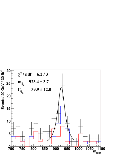
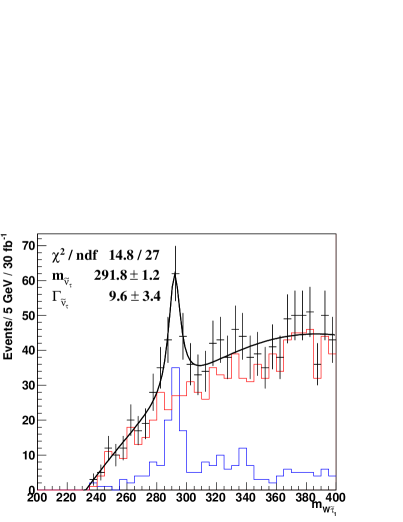
Figure 10: The jet-lepton-lepton-$\tilde{\tau}$-$\tau$ (left) and the $W$-$\tilde{\tau}$ (right) invariant-mass distributions for the $\epsilon$ benchmark point. The blue distribution is for signal events, events containing the decays of Eq. 9 and $\tilde{\nu}_{\tau}\to W\tilde{\tau}_{1}$, respectively, while the red distributions include all other events that pass the cuts given in the text.

Compared to the common mass of the first two generations of both families, $m_{\tilde{d}_{L},\tilde{s}_{L}}=938.2$ GeV and $m_{\tilde{u}_{L},\tilde{c}_{L}}=934.5$ GeV, this fit result is slightly low, indicating that there may be some systematical effect, and with a relative error of the order of 1%. However, comparing with the squark mass found in the previous Section, this analysis clearly demonstrate that there are two different masses and the decay chains allow us to assign the left- and right-handedness as we have done. Since we could not reconstruct a $\tilde{\chi}_{2}^{0}$ mass peak, the $\tilde{q}_{L}$ mass is of course also inaccessible with this technique at the $\zeta$ and $\eta$ benchmarks.

4.5 Reconstructing $\tilde{\nu}_{\tau}$ and $\tilde{\chi}^{\pm}_{1}$ Decays

The high fraction of the total cross section that comes from the associated production of $\tilde{\chi}^{\pm}_{1}\tilde{\chi}^{0}_{2}$ pairs at the $\zeta$ and $\eta$ benchmark points, together with the large production of neutralinos and charginos in the decays of squarks at all three points, makes the dominant decays of $\tilde{\chi}^{\pm}_{1}$ potentially as interesting as the $\tilde{\chi}^{0}_{2}$ decay via a left-handed slepton that was discussed in the previous Section. Accordingly, we look now at the corresponding decays of the chargino.

In the case of the $\epsilon$ benchmark point, the decay chain $\tilde{\chi}^{\pm}_{1}\to\tau\tilde{\nu}_{\tau}\to\tau W\tilde{\tau}_{1}$ has a total branching ratio of $9.5$%, and the decay $\tilde{\chi}^{0}_{2}\to\nu_{\tau}\tilde{\nu}_{\tau}\to\nu_{\tau}W\tilde{\tau}_{1}$, a branching ratio of $9.0$%. This makes the search for a $\tilde{\nu}_{\tau}$ resonance feasible, if we can reconstruct hadronic decays of the $W$ in the supersymmetric events.

The reconstruction of $W$s produced in the decays of heavy particles at the LHC is difficult because of the large jet background in the high multiplicity environment. Additionally, since $W$s will be so copiously produced in SM events at the LHC, it will be difficult to find effective background cuts. When a $W$ is produced with little boost in the laboratory frame, the jets from the decay are relatively soft and easily drown among the other jets of the event. For boosted $W$s the jets are harder, but have a much smaller opening angle in the lab frame, and are thus easily mistaken for a single jet by a cone jet algorithm. The quest for possible improvements in the search for hadronic decays of heavy bosons in supersymmetric events by the use of different jet algorithms is an interesting topic, but lies beyond the scope of this paper. As we shall see, because of the excellent rejection of the Standard Model backgrounds afforded by the properties of the stau, the identification of $W$ candidates is easier in the GDM scenarios.

To isolate events with the decay $\tilde{\nu}_{\tau}\to W\tilde{\tau}_{1}$, we apply the standard GDM cuts of Section 3, with the exception of the requirement of two tau candidates. Instead we tighten the cut on stau velocity to $\beta\gamma<2.7$, which we again find removes all SM background. This allows us a very simple identification of events with $W$s. We require one and only one combination of two jets in the event which has:

• Invariant mass within two times the width, $\Gamma_{W}=2.12$ GeV, of the $W$ mass, $m_{W}=80.42$ GeV, and

• an opening angle $\theta<\frac{\pi}{4}$ in the laboratory frame.

The cut on angle is effective in rejecting the large background of events without a $W$, where by chance two relatively soft jets have the correct invariant mass, while, for reasons discussed above, it is a typical property of $W$s that come from the decays of heavier sparticles. After these cuts and after combining the reconstructed $W$ candidates with the closest stau we arrive at the invariant mass distribution shown in Fig 10. The signal distribution (blue) shows a clear peak above the background (red), which consists mostly of events without a $W$. By fitting the total distribution with the sum of a third-degree polynomial for the background and a Breit-Wigner distribution for the peak, we arrive at a value of the tau-sneutrino mass of

$$m_{\tilde{\nu}_{\tau}}\;=\;291.8\pm 1.2~{}{\rm GeV}$$ (15)

to be compared with the nominal value of $m_{\tilde{\nu}_{\tau}}=288.5$ GeV. The overestimated value for $\epsilon$ is due to the long tails of the signal distribution to the right of the peak, which in turn comes from combinatorial effects, such as pairing the $W$ with the wrong stau candidate.

From events in the tau-sneutrino resonance peak we should in principle be able to reconstruct the chargino mass by adding tau jets to the reconstructed sneutrinos. However, the large background and the soft nature of these taus means that the signal drowns in a background of the same shape and position, much as in the case of the gluinos. For the $\zeta$ and $\eta$ benchmark points the situation is similar, we can reconstruct a $\tilde{\nu}_{\tau}$ mass peak, but no chargino. The sneutrino masses found for these points are listed in Table 3.

5 Conclusions

We have demonstrated in this paper that the LHC detectors (as exemplified here by the ATLAS detector), would have the abilities to make many valuable measurements in benchmark supersymmetric scenarios with gravitino dark matter and a $\tilde{\tau}$ NLSP. The triggers planned would record GDM events with high redundancy and efficiency, and the robust designs of the detectors would enable them to characterise very well $\tilde{\tau}$s produced in LHC collisions. Once recorded, the $\tilde{\tau}$ tracks in GDM events could be identified with high efficiency, and useful momentum, ToF and $dE/dx$ measurements would be made. We find that it should be possible to measure the stau mass with statistical and systematic errors at the sub-permille level, assuming only the reconstruction of staus with velocity down to $\beta\gamma\approx 0.6$. The majority of GDM events with a pair of $\tilde{\tau}$ NLSPs would also contain a pair of $\tau$ leptons, which should be detectable with good efficiency at the LHC. Combining these with the $\tilde{\tau}$ measurements would enable first the $\tilde{\chi}^{0}_{1}$ and subsequently heavier sparticles to be reconstructed and their masses measured with accuracies that often approach the expected systematic energy scale uncertainty of jets and leptons. We demonstrate these abilities with the aid of $\tau$ momentum recalibration using transverse momentum balance, and making appropriate kinematic cuts on the final-state kinematic distributions in sparticle cascade decays. Our results are consistent with the preliminary estimates of sparticle observability made in [20].

The LHC will be the first accelerator to explore a new energy domain, and there are high hopes that it will reveal new physics beyond the Standard Model. Supersymmetry is among the most ‘expected’ new physics surprises, which has been much studied by the LHC collaborations as well as by theorists. Most of these studies have assumed the ‘expected’ missing-energy signature of R-conserving supersymmetry with a neutralino LSP, though other possibilities have also been explored. It has been realised recently that some of these other possibilities may be as generic as missing energy, and the scenario studied here of gravitino dark matter and a stau NLSP is just one of many possible ‘unexpected’ possibilities. Nevertheless, it is encouraging that, although the LHC detectors were not designed with such an exotic scenario explicitly in mind, they seem to be capable also of dealing with such an ‘unexpected’ physics surprise. We have shown here that valuable insight into such a gravitino dark matter scenario could be obtained already with a relatively modest initial amount of LHC luminosity, and so could inform the design of possible future experiments at the high-energy frontier.