UWThPh-2006-15
Fermion masses and mixings
in a renormalizable $SO(10)\times\mathbbm{Z}_{2}$ GUT

Abstract

We investigate a scenario in a supersymmetric $SO(10)$ Grand Unified Theory in which the fermion mass matrices are generated by renormalizable Yukawa couplings of the $\mathbf{10}\oplus\mathbf{120}\oplus\overline{\mathbf{126}}$ representation of scalars. We reduce the number of parameters by assuming spontaneous CP violation and a $\mathbbm{Z}_{2}$ family symmetry, leading to nine real Yukawa coupling constants for three families. Since in the “minimal SUSY $SO(10)$ GUT” an intermediate seesaw scale is ruled out and our scenario lives in the natural extension of this theory by the $\mathbf{120}$, we identify the vacuum expectation value (VEV) $w_{R}$ of $(\mathbf{10},\mathbf{1},\mathbf{3})\in\overline{\mathbf{126}}$ with the GUT scale of $2\times 10^{16}$ GeV. In order to obtain sufficiently large neutrino masses, the coupling matrix of the scalar $\overline{\mathbf{126}}$ is necessarily small and we neglect type II seesaw contributions to the light-neutrino mass matrix. We perform a numerical analysis of this 21-parameter scenario and find an excellent fit to experimentally known fermion masses and mixings. We discuss the properties of our numerical solution, including a consistency check for the VEVs of the Higgs-doublet components in the $SO(10)$ scalar multiplets.

Introduction:

The group $SO(10)$ is a favourite candidate for constructing grand unified theories (GUTs) [1]. The special interest in such theories also stems from the fact that they allow for type I [2] and type II [3] seesaw mechanisms (see also [4]) for the light neutrino masses. Confining oneself to renormalizable $SO(10)$ GUTs, the scalar representations coupling to the chiral fermion fields, which are all assembled for each family in the 16-dimensional irreducible representation (irrep), are determined by the relation [5, 6]

$$\mathbf{16}\otimes\mathbf{16}=\left(\mathbf{10}\oplus\mathbf{126}\right)_{\mathrm{S}}\oplus\mathbf{120}_{\mathrm{AS}},$$ (1)

where the subscripts “S” and “AS” denote, respectively, the symmetric and antisymmetric parts of the tensor product. The so-called “minimal SUSY $SO(10)$ GUT” (MSGUT) [7] makes use of one $\mathbf{10}$ and one $\overline{\mathbf{126}}$ scalar irrep for the Yukawa couplings, to account for all fermion masses and mixings [8]. The MSGUT contains, in addition, one $\mathbf{210}$ and one $\mathbf{126}$ scalar irrep [7]. This model has built-in the gauge-coupling unification of the minimal SUSY extension of the Standard Model (MSSM). Detailed studies of this minimal theory have been performed [9, 10, 11, 12, 13, 14, 15, 16]; in [9, 14, 15] small effects of the 120-plet were considered in addition. It turned out that the MSGUT works surprisingly well in the fermion sector, provided one neglects constraints on the overall scale of the light neutrino masses. This, however, proved to be crucial, since the natural order of the neutrino masses in GUTs is too low, namely $v^{2}/M_{\mathrm{GUT}}\sim 1.5\times 10^{-3}$ eV, with $v\sim 174$ GeV and the GUT scale $M_{\mathrm{GUT}}\sim 2\times 10^{16}$ GeV. Thorough studies of the heavy scalar states [17, 18, 19, 20, 21, 22] have been used to show that this MSGUT is too constrained [23, 24] and does not allow to enhance the neutrino mass scale to a realistic one [25, 26], compatible with the results of the neutrino oscillation experiments (for a review see, e.g., [27]). One aspect of this problem is that a seesaw scale significantly lower than the GUT scale spoils the gauge coupling unification of the MSSM.

An obvious attempt to loosen the corset of the minimal theory is to add the 120-plet of scalars. A study in that direction has been done in [28]. Earlier works considering a prominent 120-plet contribution to the fermion mass matrices are found in [29, 30, 31, 32]. We note that $\mathbf{10}\oplus\mathbf{120}$ alone does not give a good fit in the charged fermion sector [33]. Thus the $\overline{\mathbf{126}}$ scalar irrep is not only needed in the neutrino sector but also for the charged fermion mass matrices. In that case, the mass matrices of the charged fermions and the neutrino Dirac-mass matrix are given, respectively, by

$$M_{d} = k_{d}\,H+\kappa_{d}\,G+v_{d}\,F,$$ (2)

$$M_{u} = k_{u}\,H+\kappa_{u}\,G+v_{u}\,F,$$ (3)

$$M_{\ell} = k_{d}\,H+\kappa_{\ell}\,G-3v_{d}\,F,$$ (4)

$$M_{D} = k_{u}\,H+\kappa_{D}\,G-3v_{u}\,F.$$ (5)

The Yukawa coupling matrices $H$, $G$, $F$ belong to the scalar irreps $\mathbf{10}$, $\mathbf{120}$, $\overline{\mathbf{126}}$, respectively. The coefficients $k_{d}$, $\kappa_{d}$, $\kappa_{\ell}$, $v_{d}$ denote the vacuum expectation values (VEVs) of the Higgs doublet components in the respective $SO(10)$ scalar irreps which contribute to the MSSM Higgs doublet $H_{d}$, the rest of the coefficients refers to $H_{u}$. The light neutrino mass matrix is obtained as

$$\mathcal{M}_{\nu}=M_{L}-M_{D}M_{R}^{-1}M_{D}^{T}\quad\mbox{with}\quad M_{L}=w_{L}\,F,\quad M_{R}=w_{R}\,F,$$ (6)

with scalar triplet VEVs $w_{L}$ and $w_{R}$. The mass Lagrangian of the “light” fermions reads

$$\mathcal{L}_{M}=-\bar{d}_{L}M_{d}\,d_{R}-\bar{u}_{L}M_{u}\,u_{R}-\bar{\ell}_{L}M_{\ell}\,\ell_{R}-\frac{1}{2}\bar{\nu}_{L}\mathcal{M}_{\nu}\left(\nu_{L}\right)^{c}+\mbox{H.c.},$$ (7)

with $\left(\nu_{L}\right)^{c}$ being the charge-conjugate of $\nu_{L}$.

A renormalizable $SO(10)$ scenario:

The goal of this letter is a numerical study of the system of 3-generation mass matrices (2) to (6), taking into account the neutrino-mass suppression factor $v^{2}/M_{\mathrm{GUT}}$. This system does not easily lend itself to such an investigation because it contains many parameters, thus we use some arguments to reduce their number. The scenario we want to investigate is defined by the following assumptions:

1. The Yukawa coupling matrices $H$, $G$, $F$ are real.

2. We impose a $\mathbbm{Z}_{2}$ symmetry, which sets some of the Yukawa couplings to zero and which is spontaneously broken by the VEVs of the $\mathbf{120}$, in particular, by $\kappa_{d}$, $\kappa_{u}$, $\kappa_{\ell}$, $\kappa_{D}$ being non-zero.

3. We assume $w_{R}=M_{\mathrm{GUT}}$, with $M_{\mathrm{GUT}}=2\times 10^{16}$ GeV.

4. We set $w_{L}=0$, i.e., we have pure type I seesaw mechanism.

Let us now comment on these items. Item i) can be motivated by spontaneous CP violation. The $\mathbbm{Z}_{2}$ of item ii) is given by

$$\psi_{2}\to-\psi_{2},\quad\phi_{\mathbf{120}}\to-\phi_{\mathbf{120}},$$ (8)

where the $\psi_{j}$ ($j=1,2,3$) denote the fermionic 16-plets and $\phi_{\mathbf{120}}$ is the scalar 120-plet. All other multiplets, not mentioned in Eq. (8), transform trivially. With the $\mathbbm{Z}_{2}$ symmetry of Eq. (8), the coupling matrices have the form

$$H=\left(\begin{array}[]{ccc}h_{11}&0&0\\ 0&h_{22}&0\\ 0&0&h_{33}\end{array}\right),\quad G=\left(\begin{array}[]{ccc}0&g_{12}&0\\ -g_{12}&0&g_{23}\\ 0&-g_{23}&0\end{array}\right),\quad F=\left(\begin{array}[]{ccc}f_{11}&0&f_{13}\\ 0&f_{22}&0\\ f_{13}&0&f_{33}\end{array}\right).$$ (9)

We have used the freedom of basis choice in the 1–3 sector to set $h_{13}=0$. Of course, this $\mathbbm{Z}_{2}$ symmetry of Eq. (8) is an ad-hoc symmetry, but it enhances the importance of the $\mathbf{120}$ because its Yukawa coupling matrix $G$ is now responsible for mixing of the second family with the other two. Item iii) is motivated by the fact that the MSGUT does not allow to fix the problem of too small neutrino masses by taking $w_{R}$ significantly lower than the GUT scale [23, 24, 25, 26, 28]. Thus our scenario has built in that the natural neutrino mass scale in the MSGUT is too low. Consequently, the neutrino mass scale has to be enhanced by the smallness of the coupling matrix $F$ [28]. Item iv) is a trivial consequence of the previous one: for small $F$, type II seesaw contribution to $\mathcal{M}_{\nu}$ is negligible.

Now we tackle the problem of parameter counting. Without loss of generality, we assume that $k_{d}$, $k_{u}$ and $w_{R}$ are real and positive. Then we define

$$H^{\prime}=k_{d}H,\quad G^{\prime}=\left|\kappa_{d}\right|G,\quad F^{\prime}=\left|v_{d}\right|F.$$ (10)

The primed matrices have the dimension of mass. The phases of the VEVs of the 120 and 126-plets cannot be removed. Thus we write the mass matrices as

$$M_{d} = H^{\prime}+e^{i\xi_{d}}G^{\prime}+e^{i\zeta_{d}}F^{\prime},$$ (11)

$$M_{u} = r_{H}H^{\prime}+r_{u}\,e^{i\xi_{u}}G^{\prime}+r_{F}e^{i\zeta_{u}}F^{\prime},$$ (12)

$$M_{\ell} = H^{\prime}+r_{\ell}\,e^{i\xi_{\ell}}G^{\prime}-3\,e^{i\zeta_{d}}F^{\prime},$$ (13)

$$M_{D} = r_{H}H^{\prime}+r_{D}\,e^{i\xi_{D}}G^{\prime}-3\,r_{F}e^{i\zeta_{u}}F^{\prime},$$ (14)

$$\mathcal{M}_{\nu} = r_{R}\,M_{D}{F^{\prime}}^{-1}M_{D}^{T}.$$ (15)

The ratios $r_{H}$, etc., are real by definition since we have extracted the phases from the VEVs. Now the counting is easily done. Since we have nine real Yukawa couplings, see Eq. (9), there are nine real parameters in $H^{\prime}$, $G^{\prime}$, $F^{\prime}$. Furthermore, there are six phases and six (real) ratios of VEVs, altogether 21 real parameters. On the other hand, we have 18 observables we want to fit: nine charged-fermion masses, three mixing angles and one CP phase in the CKM matrix, two neutrino mass-squared differences $\Delta m^{2}_{\mathrm{atm}}$ and $\Delta m^{2}_{\odot}$, and three lepton mixing angles.

Suppose, we have obtained a good fit for the 18 observables. Then we still have to check if the fit allows for reasonable VEVs and Yukawa coupling constants. A detailed discussion of this issue is found in Appendix A. Here it is sufficient to note that $w_{R}=M_{\mathrm{GUT}}$ and the determination of $r_{R}$ and $r_{F}$ by the fit fix $\left|v_{d}\right|$ and $\left|v_{u}\right|$ via $\left|v_{d}\right|=r_{R}M_{\mathrm{GUT}}$ and $\left|v_{u}\right|=r_{F}\left|v_{d}\right|$. Therefore, as a first test we check

$$\left|v_{d}\right|^{2}+\left|v_{u}\right|^{2}=\left|v_{d}\right|^{2}\left(1+r_{F}^{2}\right)<v^{2}\quad\mbox{with}\quad v=174\>\mathrm{GeV}$$ (16)

for every fit. Clearly, this inequality holds at the electroweak scale, and we assume that approximately it is valid at the GUT scale too.

Quarks $m_{d}$ $1.5036\!\begin{array}[]{l}\scriptstyle+0.4235\\[-8.53581pt] \scriptstyle-0.2304\end{array}$ $m_{s}$ $29.9454\!\begin{array}[]{l}\scriptstyle+4.3001\\[-8.53581pt] \scriptstyle-4.5444\end{array}$ $m_{b}$ $1063.6\!\begin{array}[]{l}\scriptstyle+141.4\\[-8.53581pt] \scriptstyle-086.5\end{array}$ $m_{u}$ $0.7238\!\begin{array}[]{l}\scriptstyle+0.1365\\[-8.53581pt] \scriptstyle-0.1467\end{array}$ $m_{c}$ $210.3273\!\begin{array}[]{l}\scriptstyle+19.0036\\[-8.53581pt] \scriptstyle-21.2264\end{array}$ $m_{t}$ $82433.3\!\begin{array}[]{l}\scriptstyle+30267.6\\[-8.53581pt] \scriptstyle-14768.6\end{array}$ $s_{12}$ $0.2243\pm 0.0016$ $s_{23}$ $0.0351\pm 0.0013$ $s_{13}$ $0.0032\pm 0.0005$ $\delta_{CKM}$ $60^{\circ}\pm 14^{\circ}$

Leptons $m_{e}$ $0.3585\!\begin{array}[]{l}\scriptstyle+0.0003\\[-8.53581pt] \scriptstyle-0.0003\end{array}$ $m_{\mu}$ $75.6715\!\begin{array}[]{l}\scriptstyle+0.0578\\[-8.53581pt] \scriptstyle-0.0501\end{array}$ $m_{\tau}$ $1292.2\!\begin{array}[]{l}\scriptstyle+0.0013\\[-8.53581pt] \scriptstyle-0.0012\end{array}$ $\Delta m^{2}_{\odot}$ $(7.9\pm 0.3)\times 10^{-5}$ $\Delta m^{2}_{\mathrm{atm}}$ $\Big{(}2.2\!\begin{array}[]{l}\scriptstyle+0.37\\[-8.53581pt] \scriptstyle-0.27\end{array}\Big{)}\times 10^{-3}$ $s_{12}^{2}$ $0.31\pm 0.025$ $s_{23}^{2}$ $0.50\pm 0.065$ $s_{13}^{2}$ $<0.0155$

Table 1: Input data at the GUT scale for $M_{\mathrm{GUT}}=2\times 10^{16}$ GeV and $\tan\beta=10$. The charged-fermion masses are taken from [35], the remaining input from Table I in [26]. Charged-fermion masses are in units of MeV, neutrino mass-squared differences in eV². We have used the abbreviations $s_{12}\equiv\sin\theta_{12}$, etc. The angles in the left table refer to the CKM matrix, in the right table to the PMNS matrix.

A numerical solution:

To find a numerical solution, we employ the downhill simplex method [34] for minimizing a $\chi^{2}$-function of the parameters—for an explanation of the method see [26, 33]. Actually, the $\chi^{2}$-function can be minimized analytically with respect to the parameter $r_{R}$ of Eq. (15), which results in a $\chi^{2}$-function depending the remaining 20 parameters, and we apply our numerical method to that function. To build in the inequality (16) in our search for the minimum, we add a suitable penalty function to our $\chi^{2}$. Our scenario is fitted against the values of the 18 observables at the GUT scale; for an MSSM parameter $\tan\beta=10$, these values are displayed in Table 1.

Choosing the normal ordering $m_{1}<m_{2}<m_{3}$ of the neutrino masses ($\Delta m^{2}_{\odot}=m_{2}^{2}-m_{1}^{2}$, $\Delta m^{2}_{\mathrm{atm}}=m_{3}^{2}-m_{1}^{2}$), we have found a fit with a $\chi^{2}=0.0087$, which is a perfect fit for all practical purposes. This fit is so good that it does not make sense to show the pulls. The matrices $H^{\prime}$, $G^{\prime}$ and $F^{\prime}$ for our fit are given by

$$H^{\prime} = \left(\begin{array}[]{ccc}0.716986&0&0\\ 0&-40.6278&0\\ 0&0&1114.41\end{array}\right),$$ (20)

$$G^{\prime} = \left(\begin{array}[]{ccc}0&7.56737&0\\ -7.56737&0&36.8224\\ 0&-36.8224&0\end{array}\right),$$ (24)

$$F^{\prime} = \left(\begin{array}[]{ccc}-0.0966851&0&4.25282\\ 0&12.3136&0\\ 4.25282&0&-61.6491\end{array}\right),$$ (28)

where all numerical values are in units of MeV; the values of the ratios of VEVs and the phases are shown in Table 2.

$r_{H}$	91.0759	-	-
-	-	$\zeta_{d}$	$19.66974^{\circ}$
$r_{F}$	297.758	$\zeta_{u}$	$-2.96594^{\circ}$
-	-	$\xi_{d}$	$189.12385^{\circ}$
$r_{u}$	7.14572	$\xi_{u}$	$226.65689^{\circ}$
$r_{\ell}$	1.33897	$\xi_{\ell}$	$6.24258^{\circ}$
$r_{D}$	3008.88	$\xi_{D}$	$179.85271^{\circ}$
$r_{R}$	$2.90553\times 10^{-17}$	-	-

Table 2: The values of the phases and ratios appearing in the mass matrices (11)–(15) in the case of our fit. Hyphens in the left two columns indicate that the ratio corresponding to the phase has been absorbed in one of the primed matrices, whereas hyphens in the right two columns signify that there is no physical phase associated with that ratio.

The neutrino mass spectrum turns out to be hierarchical with $m_{1}=1.57\times 10^{-3}\>\mbox{eV}\ll m_{2}=9.03\times 10^{-3}\>\mbox{eV}\ll m_{3}=46.96\times 10^{-3}\>\mbox{eV}$, and the PMNS phase is $12^{\circ}$. We want to stress, however, that our fit solution is perhaps not unique, because with the numerical method used here we could miss other minima of $\chi^{2}$.

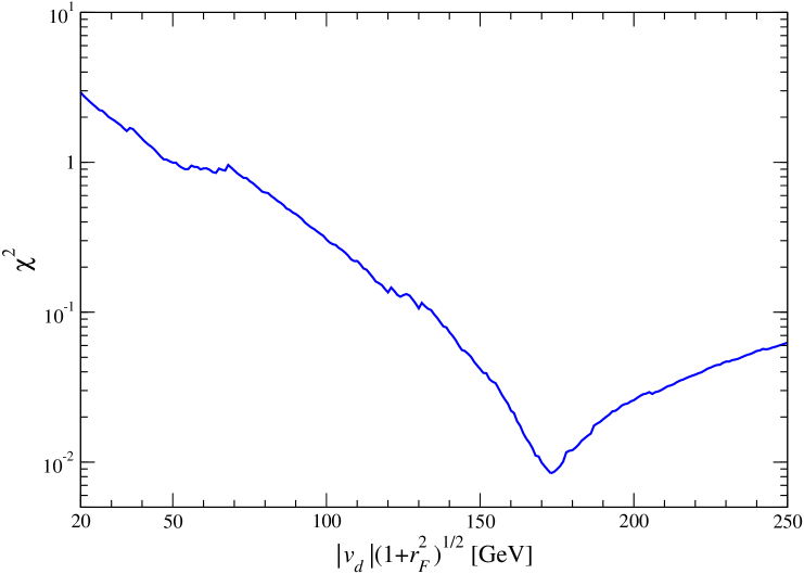
Figure 1: The $\chi^{2}$ as a function of $\left|v_{d}\right|\sqrt{1+r_{F}^{2}}$.

For our fit, it turns out that $y\equiv\left|v_{d}\right|\sqrt{1+r_{F}^{2}}=173.0$ GeV. This looks dangerously close to the upper bound of Eq. (16). To check if this danger is serious, we have plotted in Fig. 1 the minimal $\chi^{2}$ as a function of $y$. In order to pin $y$ down to a given value $\bar{y}$ we have extended the $\chi^{2}$ function to $(\chi^{2})_{y}=\chi^{2}+\left\{(y-\bar{y})/(0.01\bar{y})\right\}^{2}$, minimized $(\chi^{2})_{y}$ and plotted $\chi^{2}$ at this minimum versus $\bar{y}$—for previous uses of this method see, for instance, [26]. We read off from Fig. 1 that $\chi^{2}$ is minimal at $y=173$ GeV, however, this minimum is rather flat; note that $\chi^{2}$ is plotted on a logarithmic scale. Thus we still obtain excellent fits if we go to lower values of $y$. In Appendix A, a consistency condition is worked out which the $SO(10)$ GUT has to fulfill in order to reproduce the VEV ratios of Table 2. There we also show that for our fit all Yukawa couplings stay in the perturbative regime.

In order to find out if our scenario makes a prediction for the PMNS phase $\delta$, we treat it in the same way as $y$ in the previous paragraph, i.e., we consider $(\chi^{2})_{\delta}=\chi^{2}+\left\{(\delta-\bar{\delta})/(0.01\bar{\delta})\right\}^{2}$. Departing from $\bar{\delta}=12^{\circ}$ for our numerical solution given by Eq. (24) and Table 2, and going stepwise down close to $\bar{\delta}=0^{\circ}$ and up to $\bar{\delta}=360^{\circ}$, the quality of the fits remains excellent, with $(\chi^{2})_{\delta}$ always below 0.3. Thus, in our scenario all values of the PMNS phase are possible.

One may ask the question how large enough neutrino masses and an atmospheric mixing angle which is close to maximal are accomplished with the numerical values given by Eq. (24) and Table 2. We concentrate on achieving $\sqrt{\Delta m^{2}_{\mathrm{atm}}}\sim 0.05$ eV. With the value of $r_{R}$ we find that $r_{R}\times 10^{9}\>\mbox{MeV}\simeq 0.029\>\mbox{eV}$. Thus we take into account all contributions to $\mathcal{M}_{\nu}/r_{R}$ which are of order $10^{9}$ MeV. Rewriting Eq. (15) in the form

$$\mathcal{M}_{\nu}=r_{R}\left\{\left(r_{H}H^{\prime}+r_{D}\,e^{\xi_{D}}G^{\prime}\right){F^{\prime}}^{-1}\left(r_{H}H^{\prime}+r_{D}\,e^{i\xi_{D}}G^{\prime}\right)^{T}-6\,r_{H}r_{F}\,e^{i\zeta_{u}}H^{\prime}+9\,r_{F}^{2}\,e^{2i\zeta_{u}}F^{\prime}\right\},$$ (29)

a numerical analysis shows that all elements of the second and third term on the right-hand side are smaller than $1.8\times 10^{8}$ MeV and $0.5\times 10^{8}$ MeV, respectively. Thus the dominant matrix elements in $\mathcal{M}_{\nu}$ stem from the first term and are given by

$$\mathcal{M}_{\nu}^{(\mathrm{dom})}=r_{R}\,r_{D}\left(\begin{array}[]{ccc}0&0&0\\ 0&r_{D}\left(2g^{\prime}_{23}g^{\prime}_{12}f^{\prime}_{13}+f^{\prime}_{33}\left(g^{\prime}_{12}\right)^{2}\right)/d&-r_{H}h^{\prime}_{33}g^{\prime}_{12}f^{\prime}_{13}/d\\ 0&-r_{H}h^{\prime}_{33}g^{\prime}_{12}f^{\prime}_{13}/d&r_{D}\left(g^{\prime}_{23}\right)^{2}/f^{\prime}_{22}\end{array}\right).$$ (30)

Here, $d=f^{\prime}_{11}f^{\prime}_{33}-\left(f^{\prime}_{13}\right)^{2}$ is the determinant of the corresponding $2\times 2$ submatrix of $F^{\prime}$ and we have used the approximation $\xi_{D}=180^{\circ}$. Apart from the common factor $r_{R}$, in this matrix there are four products of three matrix elements: one matrix element is always from ${F^{\prime}}^{-1}$, the other two are either both from $r_{D}G^{\prime}$ or one from $r_{D}G^{\prime}$ and one from $r_{H}H^{\prime}$. Looking at Eq. (24) and Table 2, we find that products of the largest elements, for instance $\left(g^{\prime}_{23}\right)^{2}f^{\prime}_{33}$, never occur, these would be too large. Plugging in the numerical values of the parameters, we find that all non-zero terms in $\mathcal{M}_{\nu}^{(\mathrm{dom})}$ are similar in magnitude:

$$r_{R}\times 10^{9}\,\mbox{MeV}\,\left(\begin{array}[]{cc}(-1.77+2.64)&-0.81\\ -0.81&1.00\end{array}\right).$$ (31)

Due to the minus sign in the first term, we end up with $-1.77+2.64=0.87$, close to $1.00$ and thus leading to nearly maximal mixing. In this crude approximation, which is only relevant for the largest mass and the atmospheric mixing angle, we obtain $m_{3}\simeq 0.05$ eV and $\theta_{23}\simeq 43^{\circ}$. Apart from the smallness of $F^{\prime}$, it is the large factor $r_{D}$ in $M_{D}$ which gives the correct magnitude of the neutrino masses. Maximal atmospheric neutrino mixing rather looks like a numerical contrivance in our scenario.

Finally, a word concerning the low-energy values of the quark masses is at order. Ref. [35] takes the quark mass values at $m_{Z}$ from Ref. [37] as input for the renormalization group evolution up to $M_{\mathrm{GUT}}$, whereas Ref. [37] uses the input

$$m_{u}(1\,\mbox{GeV})=4.88\pm 0.57,\quad m_{d}(1\,\mbox{GeV})=9.81\pm 0.65,\quad m_{s}(1\,\mbox{GeV})=195.4\pm 12.5$$ (32)

and

$$m_{c}(m_{c})=1.302\begin{array}[]{c}\scriptstyle+0.037\\[-4.2679pt] \scriptstyle-0.038\end{array}\!,\quad m_{b}(m_{b})=4.34\begin{array}[]{c}\scriptstyle+0.07\\[-4.2679pt] \scriptstyle-0.08\end{array}\!,\quad m_{t}(m_{t})=171\pm 12,$$ (33)

see Tables I and II in [37]. The light quark masses are given in MeV, the heavy ones in GeV. Comparing these values with those given in the Review of Particle Properties of 2006 (RPP) [36], we find that the heavy quark masses are in reasonable agreement. However, in the last years the values of the light quark masses have become significantly lower [36]:

$$m_{u}(2\,\mbox{GeV})=1.5\div 3.0,\quad m_{d}(2\,\mbox{GeV})=3\div 7,\quad m_{s}(2\,\mbox{GeV})=95\pm 25,$$ (34)

Note that one has to take into account the scaling factor $m_{i}(1\,\mbox{GeV})/m_{i}(2\,\mbox{GeV})=1.35$ ($i=u,\,d,\,s$) to compare Eq. (32) with Eq. (34) [36]. In order to assess the influence of lowering the light quark masses, we have performed a second fit, using the values of Eq. (34) as input, scaled to $M_{\mathrm{GUT}}$ with the factor 0.200 for $m_{u}$ and 0.207 for $m_{d}$ and $m_{s}$ (see [35, 37]), but leaving the previous values for the heavy quark masses. We found an excellent fit with $\chi^{2}=0.052$, which means that our scenario is able to reproduce the lower values of the light quark masses as well. The second fit has some qualitative differences in comparison with the first one, which reinforces the suspicion that, for given input values of the 18 observables, the fit solution in our scenario is not unique.

Summary:

In this paper we have investigated fermion masses and mixings in the $SO(10)$ MSGUT, augmented by a 120-plet of scalars. The main purpose was to show that in this setting it is possible to reconcile the type I seesaw mechanism (see Eq. (6)) with a triplet VEV $w_{R}$ equal to the GUT scale of $2\times 10^{16}$ GeV, provided the theory admits that the MSSM Higgs doublet $H_{d}$ is composed mainly of the corresponding doublet components in the $\mathbf{126}$ and $\mathbf{210}$ scalar irreps—see Eq. (A11); those are the irreps which have no Yukawa couplings. This reconciliation was feasible within the scenario defined in points i)–iv), in which we have used symmetries to significantly reduce the number of degrees of freedom in the Yukawa couplings—see Eq. (9). Within this scenario we were able to find an excellent fit for all fermion masses and mixings; in this fit we have a hierarchical neutrino mass spectrum.

Thus we have obtained the following results for the minimal renormalizable $SO(10)$ GUT, with Yukawa couplings according to the relation (1):

• It is possible to reproduce the correct neutrino mass scale.

• Nevertheless, gauge coupling unification is not spoiled.

• The concrete $SO(10)$ scenario with type I seesaw mechanism, we treated in this paper, has 21 parameters, just as the MSGUT with type I+II seesaw mechanism and general complex Yukawa couplings.

It remains to be studied if our scenario allows a sufficient suppression of proton decay. In [32] it was shown that the scalar 120-plet plays a crucial role for that purpose; a certain texture of the Yukawa coupling matrices—similar to our numerical solution (24)—enables that suppression even for large $\tan\beta$.

Acknowledgments: W.G. thanks C.S. Aulakh for illuminating discussions and L. Lavoura for reading the manuscript.

Appendix A The MSSM Higgs doublets and the mass matrices

The MSSM contains two Higgs doublets, $H_{d}$ and $H_{u}$, with hypercharges $+1$ and $-1$, respectively. Their corresponding VEVs are denoted by $v\cos\beta$ and $v\sin\beta$ ($v=174$ GeV), respectively. Neglecting effects of the electroweak scale, these doublets are, by assumption, the only scalar zero modes extant at the GUT scale; this requires a minimal finetuning condition [17, 19]. The scalar irreps $\mathbf{10}$, $\overline{\mathbf{126}}$, $\mathbf{126}$, $\mathbf{210}$ contain each one doublet with the quantum numbers of $H_{d}$, whereas the $\mathbf{120}$ contains two such doublets. The $H_{d}$ is composed of these doublets [19] with the corresponding amplitudes [25] $\bar{\alpha}_{j}$ ($j=1,\ldots,6$). The analogous coefficients for $H_{u}$ are denoted by $\alpha_{j}$. The normalization conditions are

$$\sum_{j=1}^{6}\left|\alpha_{j}\right|^{2}=\sum_{j=1}^{6}\left|\bar{\alpha}_{j}\right|^{2}=1.$$ (A1)

The Dirac mass matrices, taking into account that the $\mathbf{126}$ and $\mathbf{210}$ have no Yukawa couplings, are given by

$$M_{a} = v\cos\beta\left(c^{a}_{1}\bar{\alpha}_{1}Y_{10}+c^{a}_{2}\bar{\alpha}_{2}Y_{\overline{126}}+\left(c^{a}_{5}\bar{\alpha}_{5}+c^{a}_{6}\bar{\alpha}_{6}\right)Y_{120}\right)\quad(a=d,\ell),$$ (A2)

$$M_{b} = v\sin\beta\left(c^{b}_{1}\alpha_{1}Y_{10}+c^{b}_{2}\alpha_{2}Y_{\overline{126}}+\left(c^{b}_{5}\alpha_{5}+c^{b}_{6}\alpha_{6}\right)Y_{120}\right)\quad(b=u,D),$$ (A3)

with Yukawa coupling matrices $Y_{10}$, $Y_{\overline{126}}$, $Y_{120}$ and Clebsch-Gordan coefficients $c^{a,b}_{j}$ deriving from the $SO(10)$-invariant Yukawa couplings [20, 23]. The absolute values of the Clebsch-Gordan coefficients have no physical meaning and some of their phases are convention-dependent. With our conventions, the required information reads

$$\begin{array}[]{l}c^{d}_{1}=c^{u}_{1}=c^{\ell}_{1}=c^{D}_{1},\\ c^{d}_{2}=-c^{u}_{2}=-\frac{1}{3}\,c^{\ell}_{2}=\frac{1}{3}\,c^{D}_{2},\\ c^{d}_{5}=-c^{u}_{5}=c^{\ell}_{5}=-c^{D}_{5},\\ c^{d}_{6}=c^{u}_{6}=-\frac{1}{3}\,c^{\ell}_{6}=-\frac{1}{3}\,c^{D}_{6},\\ c^{d}_{5}/c^{d}_{6}=\sqrt{3}.\end{array}$$ (A4)

Equations (A2) and (A3) together with this equation lead to the mass matrices (2)–(5). Furthermore, comparing Eqs. (A2) and (A3) with Eq. (10), we find

$$H^{\prime}=v\cos\beta\,c^{d}_{1}\left|\bar{\alpha}_{1}\right|Y_{10},\quad F^{\prime}=v\cos\beta\,c^{d}_{2}\left|\bar{\alpha}_{2}\right|Y_{\overline{126}},\quad G^{\prime}=v\cos\beta\left|c^{d}_{5}\bar{\alpha}_{5}+c^{d}_{6}\bar{\alpha}_{6}\right|Y_{120}.$$ (A5)

Comparison with Eqs. (11)–(14) and using Eq. (A4) delivers the coefficients

$$r_{H}=\tan\beta\left|\frac{\alpha_{1}}{\bar{\alpha}_{1}}\right|, \displaystyle r_{F}=\tan\beta\left|\frac{\alpha_{2}}{\bar{\alpha}_{2}}\right|,$$ (A6)

$$r_{u}=\tan\beta\left|\frac{\alpha_{6}-\sqrt{3}\,\alpha_{5}}{\bar{\alpha}_{6}-\sqrt{3}\,\bar{\alpha}_{5}}\right|, \displaystyle r_{\ell}=\left|1-\frac{2\,\bar{\alpha}_{6}}{\bar{\alpha}_{6}-\sqrt{3}\,\bar{\alpha}_{5}}\right|, r_{D}=\tan\beta\left|\frac{3\,\alpha_{6}+\sqrt{3}\,\alpha_{5}}{\bar{\alpha}_{6}-\sqrt{3}\,\bar{\alpha}_{5}}\right|.$$ (A7)

Now we want to check the consistency of our numerical solution given by Eq. (24) and Table 2. From $r_{D}\gg r_{u}$, it follows that

$$\sqrt{3}\,\alpha_{5}\simeq\alpha_{6}\simeq\frac{r_{D}}{4\,\tan\beta}\left|\bar{\alpha}_{6}-\sqrt{3}\,\bar{\alpha}_{5}\right|.$$ (A8)

Furthermore, using $r_{\ell}\sim 1$, we find the order-of-magnitude relations

$$\bar{\alpha}_{5}\sim\bar{\alpha}_{6}\sim\tan\beta/r_{D}.$$ (A9)

Then the first of the normalization conditions (A1) reads approximately

$$\sum_{j}\left|\alpha_{j}\right|^{2}\simeq\frac{1}{\tan^{2}\beta}\left(r_{H}^{2}\left|\bar{\alpha}_{1}\right|^{2}+r_{F}^{2}\left|\bar{\alpha}_{2}\right|^{2}+\frac{1}{12}\,r_{D}^{2}\left|\bar{\alpha}_{6}-\sqrt{3}\,\bar{\alpha}_{5}\right|^{2}\right)+\left|\alpha_{3}\right|^{2}+\left|\alpha_{4}\right|^{2}\simeq 1.$$ (A10)

This means that $\left|\bar{\alpha}_{j}\right|^{2}\ll 1$ for $j=1,2,5,6$. Therefore, the second normalization condition is given by

$$\sum_{j}\left|\bar{\alpha}_{j}\right|^{2}\simeq\left|\bar{\alpha}_{3}\right|^{2}+\left|\bar{\alpha}_{4}\right|^{2}\simeq 1,$$ (A11)

and the brunt of the normalization has to be supplied by the components of $H_{d}$ in the $\mathbf{126}$ and $\mathbf{210}$, which do not couple to the fermions. This is a consistency condition for the scenario presented in this paper.

To translate the condition (16) into the formalism presented here, we note that $\left|v_{d}\right|^{2}\ll\left|v_{u}\right|^{2}$ and $\sin\beta\simeq 1$ for $\tan\beta=10$. Therefore, Eq. (16) effectively checks if the necessary condition $\left|\alpha_{2}\right|<1$ is fulfilled.

Finally, it remains to see if our numerical solution respects the perturbative regime of the Yukawa sector. It suffices to consider the largest elements of the Yukawa couplings

$$Y_{d}=\frac{1}{v\cos\beta}\,M_{d},\quad Y_{u}=\frac{1}{v\sin\beta}\,M_{u},\quad Y_{\ell}=\frac{1}{v\cos\beta}\,M_{\ell},\quad Y_{D}=\frac{1}{v\sin\beta}\,M_{D},$$ (A12)

which reside in $Y_{u}$ and $Y_{D}$. The largest entry in $Y_{u}$ is the 33-element with the main contribution from $r_{H}h^{\prime}_{33}/(v\sin\beta)\simeq 0.59$. The 23-element with $r_{D}g^{\prime}_{23}/(v\sin\beta)\simeq 0.64$ dominates in $Y_{D}$. These numbers demonstrate that for our numerical solution the Yukawa couplings remain in the perturbative regime.

References

- [1] H. Fritzsch, P. Minkowski, Ann. Phys. 93 (1975) 193.
-
[2]
P. Minkowski,
Phys. Lett. B 67 (1977) 421;
T.Yanagida, in Proceedings of the Workshop on Unified Theory and Baryon Number in the Universe, O. Sawata and A. Sugamoto eds., KEK report 79-18, Tsukuba, Japan, 1979;
S.L. Glashow, in Quarks and Leptons, Proceedings of the Advanced Study Institute (Cargèse, Corsica, 1979), J.-L. Basdevant et al. eds., Plenum, New York, 1981;
M. Gell-Mann, P. Ramond, and R. Slansky, in Supergravity, D.Z. Freedman and F. van Nieuwenhuizen eds., North Holland, Amsterdam, 1979;
R.N. Mohapatra, G. Senjanović, Phys. Rev. Lett. 44 (1980) 912. -
[3]
G. Lazarides, Q. Shafi, C. Wetterich,
Nucl. Phys. B 181 (1981) 287;
R.N. Mohapatra, G. Senjanović, Phys. Rev. D 23 (1981) 165;
R.N. Mohapatra, P. Pal, Massive Neutrinos in Physics and Astrophysics, World Scientific, Singapore, 1991, p. 127. -
[4]
J. Schechter, J.W.F. Valle,
Phys. Rev. D 22 (1980) 2227;
S.M. Bilenky, J. Hošek, S.T. Petcov, Phys. Lett. 94B (1980) 495;
I.Yu. Kobzarev, B.V. Martemyanov, L.B. Okun, M.G. Shchepkin, Yad. Phys. 32 (1980) 1590 [Sov. J. Nucl. Phys. 32 (1981) 823];
J. Schechter, J.W.F. Valle, Phys. Rev. D 25 (1982) 774. - [5] R.N. Mohapatra, B. Sakita, Phys. Rev. D 21 (1980) 1062.
- [6] R. Slansky, Phys. Rep. 79 (1981) 1.
-
[7]
C.S. Aulakh, R.N. Mohapatra,
Phys. Rev. D 28 (1983) 217;
T.E. Clark, T.K. Kuo, N. Nakagawa, Phys. Lett 115B (1982) 26;
C.S. Aulakh, B. Bajc, A. Melfo, G. Senjanović, F. Vissani, Phys. Lett. B 588 (2004) 196 [hep-ph/0306242]. - [8] K.S. Babu, R.N. Mohapatra, Phys. Rev. Lett. 70 (1993) 2845 [hep-ph/9209215].
- [9] K. Matsuda, T. Fukuyama, H. Nishiura, Phys. Rev. D 61 (2000) 053001 [hep-ph/9906433].
-
[10]
K. Matsuda, Y. Koide, T. Fukuyama,
Phys. Rev. D 64 (2001) 053015
[hep-ph/0010026];
K. Matsuda, Y. Koide, T. Fukuyama, H. Nishiura, Phys. Rev. D 65 (2002) 033008 (Erratum-ibid. D 65 (2002) 079904) [hep-ph/0108202]. - [11] T. Fukuyama, N. Okada, JHEP 11 (2002) 011 [hep-ph/0205066].
-
[12]
B. Bajc, G. Senjanović, F. Vissani,
Phys. Rev. Lett. 90 (2003) 051802
[hep-ph/0210207];
B. Bajc, G. Senjanović, F. Vissani, Phys. Rev. D 70 (2004) 093002 [hep-ph/0402140]. -
[13]
H.S. Goh, R.N. Mohapatra, S.P. Ng,
Phys. Lett. B 570 (2003) 215
[hep-ph/0303055];
H.S. Goh, R.N. Mohapatra, S.P. Ng, Phys. Rev. D 68 (2003) 115008 [hep-ph/0308197]. - [14] S. Bertolini, M. Frigerio, M. Malinský, Phys. Rev. D 70 (2004) 095002 [hep-ph/0406117].
- [15] S. Bertolini, M. Malinský, Phys. Rev. D 72 (2005) 055021 [hep-ph/0504241].
- [16] K.S. Babu, C. Macesanu, Phys. Rev. D 72 (2005) 115003 [hep-ph/0505200].
- [17] C.S. Aulakh, A. Girdar, Int. J. Mod. Phys. A 20 (2005) 865 [hep-ph/0204097].
- [18] T. Fukuyama, A. Ilakovac, T. Kikuchi, S. Meljanac, N. Okada, Eur. Phys. J. C 42 (2005) 191 [hep-ph/0401213].
- [19] B. Bajc, A. Melfo, G. Senjanović, F. Vissani, Phys. Rev. D 70 (2004) 035007 [hep-ph/0402122].
- [20] C.S. Aulakh, A. Girdar, Nucl. Phys. B 711 (2005) 275 [hep-ph/0405074].
-
[21]
T. Fukuyama, A. Ilakovac, T. Kikuchi, S. Meljanac, N. Okada,
J. Math. Phys. 46 (2005) 033505
[hep-ph/0405300];
T. Fukuyama, A. Ilakovac, T. Kikuchi, S. Meljanac, N. Okada, Phys. Rev. D 72 (2005) 051701 [hep-ph/0412348]. - [22] C.S. Aulakh, Phys. Rev. D 72 (2005) 051702 [hep-ph/0501025].
- [23] C.S. Aulakh, expanded version of the plenary talks at the Workshop Series on Theoretical High Energy Physics, IIT Roorkee, Uttaranchal, India, March 16–20, 2005, and at the 8th European Meeting “From the Planck Scale to the Electroweak Scale” (PLANCK05), ICTP, Trieste, Italy, May 23–28, 2005, hep-ph/0506291.
- [24] B. Bajc, A. Melfo, G. Senjanović, F. Vissani, Phys. Lett. B 634 (2006) 272 [hep-ph/0511352].
- [25] C.S. Aulakh, S.K. Garg, hep-ph/0512224.
- [26] S. Bertolini, T. Schwetz, M. Malinský, Phys. Rev. D 73 (2006) 115012 [hep-ph/0605006].
- [27] M. Maltoni, T. Schwetz, M.A. Tórtola, J.W.F. Valle, New. J. Phys. 6 (2004) 122 [hep-ph/0405172].
- [28] C.S. Aulakh, hep-ph/0602132.
-
[29]
N. Oshimo,
Phys. Rev. D 66 (2002) 0950
[hep-ph/0206239];
N. Oshimo, Nucl. Phys. B 668 (2003) 258 [hep-ph/0305166]. - [30] Wei-Min Yang, Zhi-Gang Wang, Nucl. Phys. 707 (2005) 87 [hep-ph/0406221].
- [31] B. Dutta, Y. Mimura, R.N. Mohapatra, Phys. Lett. B 603 (2004) 35 [hep-ph/0406262].
-
[32]
B. Dutta, Y. Mimura, R.N. Mohapatra,
Phys. Rev. Lett. 94 (2005) 091804
[hep-ph/0412105];
B. Dutta, Y. Mimura, R.N. Mohapatra, Phys. Rev. D 72 (2005) 075009 [hep-ph/0507319]. - [33] L. Lavoura, H. Kühböck, W. Grimus, Nucl. Phys. B 754 (2006) 1 [hep-ph/0603259].
-
[34]
J.A. Nelder, R. Mead,
Comp. J. 7 (1965) 306;
W.H. Press, B.P. Flannery, S.A. Teukolsky, and W.T. Vetterling, Numerical recipes in C: The art of scientific computing, Cambridge University Press, 1992. - [35] C.R. Das, M.K. Parida, Eur. Phys. J. C 20 (2001) 121 [hep-ph/0010004].
- [36] W.-M. Yao et al., Review of Particle Physics, J. Phys. G 33 (2006) 1.
- [37] H. Fusaoka, Y. Koide, Phys. Rev. D 57 (1998) 3986 [hep-ph/9712201].