Dynamical chiral symmetry breaking with Minkowski space integral representations

Abstract

The fermion propagator is studied in the whole Minkowski space with the help of the Schwinger-Dyson equations. Various integral representations are employed to get solutions for the dynamical breaking of chiral symmetry in different regimes of the coupling constant. In particular, in the case of massive boson, we extend the singularity structure of the fermion propagator to the two real pole Ansatz.

In this brief report we investigate a possible scenario of dynamical mass generation and estimate the timelike structure of the fermion propagator. This phenomenon, dubbed also as dynamical chiral symmetry breaking, requires intrinsically non-perturbative tools since the particle masses can be fully generated via loop contributions. In the framework of Schwinger-Dyson equations (SDEs) we explore the fermion mass function and the fermion propagator in Minkowski space. We develop a novel integral technique to solve with reasonable precision a SDE which has only been addressed at one-loop order BICUDO (for Yukawa model). Here, we consider a gauge theory and resort to a simple quenched approximation with the massive gauge boson transverse mode. The effective coupling is then regulated by a Pauli-Villars cutoff $\Lambda$.

The main result of this paper is to show that for the scaling $M/\Lambda<<1$ (walking Technicolor) the analytical structure of the exact propagator is given the Lehmann representation with one real pole in this propagator. Increasing the ratio $M/\Lambda$, we explicitly show that two pole Ansatz plus the corresponding generalized integral representation for the exact propagator is fully adequate for the description of dynamical chiral symmetry breaking in this phase. The novel integral representation which goes beyond the Lehmann representation is introduced for this purpose. Within the presented framework we achieve larger value of the scaling $M/\Lambda\simeq 0.1$.

In a parity conserving theory the general form of the fermion propagator reads

$$S(p)=\frac{F(p^{2})}{\not p-M(p^{2})}\,.$$ (1)

For simplicity we assume $F(p^{2})=1$, which is reasonable approximation for gauge theories in the Landau gauge. The SDE for the mass function $M$ is modeled in the following manner

$$M(p^{2})=S^{-1}_{0}(p)-S^{-1}(p)=ig^{2}\int\frac{d^{4}q}{(2\pi)^{4}}\gamma^{\alpha}S(q)\gamma^{\beta}$$

$$\left[-g^{\alpha\beta}+\frac{l_{\alpha}l_{\beta}}{l^{2}}\right]\left[\frac{1}{l^{2}-m_{B}^{2}+i\epsilon}-\frac{1}{l^{2}-{\Lambda}^{2}+i\epsilon}\right]\,,$$

where $l=p-q$, the constant $g^{2}$ implicitly absorbs a possible group prefactor, and $S_{0}(p)$ represents the free fermion propagator. In such approximation the effective coupling does not run logarithmically, but it is constant up to a scale $\Lambda$ where it rapidly vanishes (i.e. it runs with power behaviour). Notice that in what concerns QCD, lowering the cutoff to the scale of $\Lambda_{QCD}\simeq 250$ MeV and keeping the coupling large enough such that constituent (infrared) quark mass $M\simeq\Lambda$ can be regarded as an approximation of QCD, while when $M<<\Lambda$, the limit of walking Technicolors is modeled HOLDOM1985 ; YABAMA1986 , for a recent treatment within the SDEs framework see JAPONCI .

A little is known about the full Minkowski solution of SDEs in strong coupling field theories, hence we can refer here the paper of Fukuda and Kugo FUKKUG Furthermore, the timelike structure of Greens function as it is read from the Euclidean counterparts is not reliably known FISCHER . The main aim of this report is to present the direct solutions in Minkowski space, assuming a spectral and a generalized integral representation of the propagator for this purpose.

In order to carefully compare our Minkowski solutions with the spacelike part obtained independently in Euclidean space, we also perform the Wick rotation $iq_{0}\rightarrow q_{4}$ and solve SDE in Euclidean space After the angular integration the Euclidean SDE reads MANA1974 ,

$$M(p_{E}^{2})=\frac{3\alpha}{8\pi}\,\int_{0}^{\infty}dq^{2}_{E}\,\frac{M(q^{2}_{E})\left[B(q,p,m_{B})-B(q,p,\Lambda)\right]}{p_{E}^{2}\left[q^{2}_{E}+M^{2}(q_{E}^{2})\right]}$$

$$B(q,p,x)=-x^{2}+\sqrt{\lambda(-p^{2}_{E},-q^{2}_{E},x^{2})}\,,$$ (2)

where $q^{2}_{E}=-q^{2}$ (and similarly for $p$), $\alpha=g^{2}/(4\pi)$ and the symbol $\lambda$ stands for the triangle Källen function, $\lambda(x,y,z)=(x-y-z)^{2}-4yz$ .

The solution of the Eq.  (Dynamical chiral symmetry breaking with Minkowski space integral representations) is well known: for the coupling below certain critical value $\alpha_{c}$ there exists only a trivial solution $M(p_{E}^{2})=0$, while for $\alpha>\alpha_{c}$ we get a non-trivial mass function. The value of the critical coupling $\alpha_{c}$ depends on the details of the kernel, especially on the finite ratio $R=m_{B}/\Lambda$, noting that for $m_{B}<<\Lambda$ the critical coupling constant $\alpha_{c}\simeq\pi/3$ coincides with the one obtained in the ladder approximation for the electron propagator in the strong coupling QED, where the well-known exponential Miransky scaling is exhibited:

$$M(0)\simeq const\cdot\Lambda e^{-\left[\pi(\alpha/\alpha_{c}-1)^{-1/2}\right]}\,.$$ (3)

In the first part of our SDE Minkowski study we assume spectral representation with a single real pole in the propagator and derive the Unitary Equations in their full non-linearized form. The solutions of Schwinger-Dyson equations obtained by the spectral method has been already calculated for several models LACO ; SAULIJHEP . Stressed that in any case, the resulting spacelike parts of Greens functions under consideration LACO ; SAULIJHEP , were in a good agreement with the solutions based on the Euclidean formalism.

Assumed Lehmann spectral representation reads,

$$S(p)=\int_{R^{+}}dx\,\frac{\not p\sigma_{v}(x)+\sigma_{s}(x)}{p^{2}-x+i\epsilon}\,,$$ (4)

where $S$ has a pole at $p^{2}=m^{2}$, i.e., $\sigma_{s}(x)=rm\delta(x-m^{2})+\sigma_{s}^{c}(x)$, where $r$ represents the residuum. The function $\sigma_{s}^{c}(x)$ is a continuous part of the spectral function starting to be non-zero from the first branch point. Substituting the integral representation (4) into our gap equation written in Minkowski space,

$$M(p^{2})=i3g^{2}\int dx\int\frac{d^{4}q}{(2\pi)^{4}}G(p-q)\frac{\sigma_{s}(x)}{q^{2}-x+i\epsilon}\,,$$ (5)

one arrives to the following dispersion relation for the mass function $M$,

$$M(p^{2})=\int d\omega\frac{\rho_{s}(\omega)}{p^{2}-\omega+i\epsilon}\,,$$ (6)

$$\rho_{s}(\omega)=\frac{\alpha}{(4\pi)}\int dx\sigma_{s}(x)\left[X_{0}(\omega;m_{B}^{2},x)-X_{0}(\omega;\Lambda^{2},x)\right]\,,$$

$$X_{0}(\omega;a,b)=\frac{\sqrt{\lambda(\omega,a,b)}}{\omega}\Theta\left(\omega-(\sqrt{a}-\sqrt{b})^{2}\right)\,.$$

The imaginary part of the propagator and the imaginary part of the dynamical mass function are simply related, this relation closes the system of the equations (6) employed. In our approximation $Z=1$ and it is sufficient to consider the $S_{s}$ part of the propagator,

$$S_{s}(p^{2}) = \frac{M(p^{2})}{p^{2}-M^{2}(p^{2})}$$ (7)

$$= \Sigma_{R}\frac{p^{2}-\Sigma_{R}^{2}-\Sigma_{I}^{2}}{\left(p^{2}-\Sigma_{R}^{2}+\Sigma_{I}^{2}\right)^{2}+4\Sigma_{R}^{2}\Sigma_{I}^{2}}$$

$$+ i\,\Sigma_{I}\frac{p^{2}+\Sigma_{R}^{2}+\Sigma_{I}^{2}}{\left(p^{2}-\Sigma_{R}^{2}+\Sigma_{I}^{2}\right)^{2}+4\Sigma_{R}^{2}\Sigma_{I}^{2}}$$

where we use a shorthand notation, $\Sigma_{R}={\rm Re}\ M(p^{2})\,;\Sigma_{I}={\rm Im}\ M(p^{2})=-\pi\rho(p^{2})$. Comparing imaginary part of (7) with the imaginary part of the propagator ${\rm Im}\,S_{s}(p^{2})=-\pi\sigma_{s}^{c}(p^{2})$, we immediately get

$$\sigma_{s}^{c}(p^{2})=\rho_{s}(p^{2})\frac{p^{2}+\Sigma_{R}^{2}+\Sigma_{I}^{2}}{\left(p^{2}-\Sigma_{R}^{2}+\Sigma_{I}^{2}\right)^{2}+4\Sigma_{R}^{2}\Sigma_{I}^{2}}\,,$$ (8)

which is nonzero for time-like momenta above the threshold. The derivation of more general “Unitary equations” which takes into account the wave function renormalization is straightforward (see for instance LACO ).

The dispersive (real) part of the mass functions is given by the principal value integral

$$\Sigma_{R}(p^{2})=P\cdot\int d\omega\frac{\rho_{s}(\omega)}{p^{2}-\omega}\,.$$ (9)

The principal value can be avoided by using $\rho$ as given in (6), which yields an ordinary regular integral over the new kernel,

$$\Sigma_{R}(p^{2})=\frac{3\alpha}{4\pi}\int dx\sigma_{s}(x)\left[J(p^{2},x,m_{B}^{2})-J(p^{2},x,\Lambda^{2})\right]\,,$$

where $J$ results from the principal value integration of the dispersion relation for $M$,

$$J(p^{2},x,z)=-\frac{\Theta(-\lambda_{p})\sqrt{-\lambda_{p}}}{p^{2}}\left[\frac{\pi}{2}+{\rm arctg}\frac{p^{2}-x-z}{\sqrt{-\lambda_{p}}}\right]$$

$$-\frac{\Theta(\lambda_{p})\sqrt{(}\lambda_{p})}{p^{2}}\ln\left|\frac{p^{2}-x-z+\frac{\lambda_{p}}{(\sqrt{x}+\sqrt{z})^{2}-p^{2}}}{p^{2}-x-z+\sqrt{\lambda_{p}}}\right|+$$

$$\frac{\Theta(\lambda_{0})\sqrt{\lambda_{0}}}{p^{2}}\ln\left|\frac{-x-z+\frac{\lambda_{0}}{(\sqrt{x}+\sqrt{z})^{2}}}{-x-z+\sqrt{\lambda_{0}}}\right|+\frac{1}{2}\ln(16xz)\,,$$

where we have shortly written $\lambda_{p,(0)}=\lambda(p^{2}(0),x,z)$.

The residuum $r$ and the pole mass function $m$ are obtained evaluating the dispersion relation and its derivative. The coupled set of the integral equations above has been solved numerically by iterations.

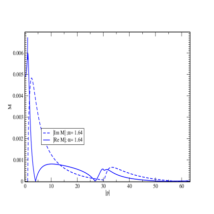
Figure 1: Absolute value of the mass function at time-like momenta with single pole in the propagator.

The Unitary equations provide solutions for time-like momenta above the branch point $p^{2}>(m_{B}+m)^{2}$, below which the propagator is real. The results on the negative axis of $p^{2}$ are easily obtained by a regular integration either from (6) or from the dispersion relation for $M$ (4). The resulting timelike solution is presented in Fig. 1). The results presented here are calculated with ${\Lambda}/{m_{B}}=30$.

and we use the mass $m_{B}$ as a scale for all dimensionfull quantities. The comparison of spectral Minkowski and Euclidean solutions is shown in Fig. 2. Thus, solving the Unitary Equations and comparing the Minkowski solution to the Euclidean one, we find rather nice agreement near the critical coupling. However, when the coupling becomes larger (say when $\alpha$ exceeds $\alpha_{c}$, about $\alpha$ 10 %) a discrepancy appears, since the employed spectral representation for the propagator, with just one pole, is no longer valid. Retrospectively, the previous one loop analytical calculations BICUDO already found evidence for a more complex structure in the propagator. Apparently new singularities appear in the propagator for $\alpha>\alpha_{T}\,$ The coupling $\alpha_{T}$ was determined to be $\,\alpha_{T}=1.73\pm 0.02$ in our case. .

In what follows we continue with our study of the SDE in Minkowski space relaxing our assumption on the spectral representation of the fermion propagator.

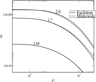
Figure 2: Dynamical mass function for space-like momenta for various coupling $\alpha=1.64;\,1.7,\,2.0$. Solid (dashed) lines stand for Euclidean (Minkowski) solutions.

The reason for the fail of one pole Ansatz is easy to understand: the dynamical mass is an increasing function in the regime from $p^{2}=0$ to the branch point $p_{B}^{2}=(m+m_{B})^{2}$. When the coupling is large enough, then the large enhancement below the branch point maintains and the dynamical mass function necessarily crosses the line $\sqrt{p^{2}}$. Thus, for a certain set of parameters the propagator develops two real poles which should be taken into account in the integral Ansatz. The second real pole first appears at the branch point $p_{B}^{2}=(m+m_{B})^{2}$ and moves down towards the first one as the coupling increases. To get a better view we draw this scenario in in Fig. 3. The lines displayed represent our numerical findings.

The new integral Ansatz, which is consistent with the solution of SDE in the regime where the two poles are present, reads

$$S_{s}(p^{2}) = \frac{m_{-}}{p^{2}-m^{2}_{+}+i0}-\frac{m_{-}}{p^{2}-m^{2}_{-}+i0}$$ (10)

$$+ \frac{1}{p^{2}-m^{2}_{-}+i0}\int d\omega\frac{\sigma_{s}^{-}(\omega)}{p^{2}-\omega+i0}\ .$$

The alternative equivalent representation can be obtained by replacements $m_{-}\rightarrow-m_{+},\sigma_{s}^{-}\rightarrow\sigma_{s}^{-}$.

This Ansatz immediately implies the dispersive relation for the dynamical mass function. Taking $F=1$ approximation again and substituting the formula (10) into the SDE it leads after the integration over the momenta to the following result for the function $\rho_{s}(p^{2})$

$$- \rho_{s}(\omega)\frac{(4\pi)^{2}}{g^{2}}=m_{-}\left[X_{0}(\omega;m_{+}^{2},m_{B}^{2})-X_{0}(\omega;m_{+}^{2},\Lambda^{2})\right.$$ (11)

$$-\left.X_{0}(\omega;m_{-}^{2},m_{B}^{2})+X_{0}(\omega;m_{-}^{2},\Lambda^{2})\right]$$

$$+ \int dx\,\frac{\sigma_{s}^{-}(x)}{m_{-}^{2}-x}\left[X_{0}(\omega;m_{-}^{2},m_{B}^{2})-X_{0}(\omega;{\Lambda}^{2},m_{-}^{2})\right]$$

$$-\int dx\frac{\sigma_{s}^{-}(x)}{m_{-}^{2}-x}\left[X_{0}(\omega;m_{B}^{2},x)-X_{0}(\omega;{\Lambda}^{2},x)\right]\,,$$

where the first line in (11) follows from the first two terms in (10) and the second line follows from the third term in (10). The derivation of (11) is straightforward and follows the same lines as in the case of the standard Lehmann representation. The integration over the momentum is finite and it remains finite even when $\Lambda$ is sent to infinity, which is a consequence of the momentum behavior of our Ansatz (10).

The Unitary equations are modified since the integral representation has changed. To derive them let us compare the imaginary and the real parts of the propagator above the branch point $(m_{B}+m_{+})^{2}$ (by definition, $m_{-}>m_{+}$).

On one side we get from the imaginary part of (10)

$${\rm Im}\,S_{s}(p^{2})=-\frac{\pi\sigma_{s}^{-}(p^{2})}{p^{2}-m_{-}^{2}}$$ (12)

and the imaginary part of this function, computed with the SDE, is still given by Eq. (7). This implies that $S_{s}$ is real up to the $p^{2}=(m_{-}+m_{B})^{2}$.

Thus we get for the time-like momenta, such that $p^{2}>(m_{-}+m_{B})^{2}$, the following equation,

$$\sigma_{s}^{-}(p^{2})=\rho(p^{2})\frac{(p^{2}-m_{-}^{2})(p^{2}+\Sigma_{R}^{2}+\Sigma_{I}^{2})}{\left(p^{2}-\Sigma_{R}^{2}+\Sigma_{I}^{2}\right)^{2}+4\Sigma_{R}^{2}\Sigma_{I}^{2}}\,.$$ (13)

This means that the momentum space Schwinger-Dyson equation turns into two coupled regular equations (11) and (13) relating the absorptive and dispersive parts of the propagator and its inverse.

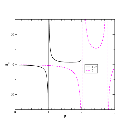
Figure 3: (Color online) Propagator singularities bellow threshold shown for two different coupling constant. The dashed (solid) line stands for the case when the propagator function $S_{s}$ exhibits two (one) real poles below the branch points.

The pole masses are necessarily expected below the threshold and they are determined by the zeroes of the inverse of the propagator i.e., $m_{\pm}=M(m_{\pm}^{2})\,$ . The real part of the mass $\Sigma_{R}$ entering Eq. (13) is given by the principal value integration over $\rho$ in Eq. (11) . This leads to the following compact regular integral equation for $\Sigma_{R}$,

$$- \Sigma_{R}(p^{2})\frac{(4\pi)^{2}}{g^{2}}=m_{-}\left[J(p^{2},m_{-}^{2},m_{B}^{2})-J(p^{2},m_{-}^{2},\Lambda^{2})\right.$$ (14)

$$\left.-J(p^{2},m_{+}^{2},m_{B}^{2})+J(p^{2},m_{+}^{2},\Lambda^{2})\right]$$

$$+ \int dx\,\frac{\sigma_{s}^{-}(x)}{m_{-}^{2}-x}\left[J(p^{2},m_{-}^{2},m_{B}^{2})-J(p^{2},m_{-}^{2},{\Lambda}^{2})\right.$$

$$-\left.J(p^{2},x,m_{B}^{2})+J(p^{2},x,\Lambda^{2})\right]\,.$$

The second pole appears for couplings stronger than $\alpha_{T}\simeq 1.73$. In the interval of the couplings $1.73<\alpha<2.0$ the two-pole representation of the propagator leads to solutions which, for space-like momenta, agree rather well with the Euclidean ones.

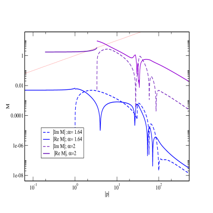
Figure 4: (Color online) Absolute value of the mass function at time-like regime of the momenta in log-log plot. The upper two lines represent the real and imaginary parts of the mass function $M$ for $\alpha=2$, the two lines below coincide with the data plotted in Fig. 2.

Our solution for the coupling $\alpha=2$ is added in the Fig. 2 for spacelike and it is displayed in the Fig.  4 for timelike momenta. Our Minkowski solution becomes unstable for $\alpha>2$ and starts to disagree with the spacelike Euclidean results for $\alpha>2$. To dive more deep into the chiral breaking phase and thus achieve enhancement of the infrared mass would require a new reanalysis of up to now unknown, possibly complex, propagator singularities.

To conclude, the one-pole case is adequate to solve dynamical chiral symmetry breaking near to the critical coupling, while the two pole fit is adequate to work with moderate couplings, well into the phase transition region where the standard spectral representation deviates from the correct solution. For the later case, a suitable integral representation of the propagator has been proposed.

References

(1)
P. Bicudo, Phys. Rev. D69, 074003 (2004).
(2)
B. Holdom, Phys. Lett. B150, 301 (1985).
(3)
K. Yamawaki, M. Bando, and K. Matumato,
Phys. Rev. Lett. 56, 1335 (1986).
(4)
M. Harada, M. Kurachi, K. Yamawaki,Phys. Rev. D68, 076001 (2003);
M. Kurachi and R. Shrock, JHEP 0612, 034 (2006).
(5)
T. Maskawa and H. Nakajima,
Prog. Theor. Phys. 52, 1326 (1974).
(6)
R. Fukuda, T. Kugo, Nucl. Phys. B 117, 250 (1976).
(7)
R. Alkofer, W. Detmold, C.S. Fischer, P. Maris,
Phys. Rev. D70, 014014 (2004).
(8)
V. Šauli, Few Body Systems39, 1-2, hep-ph/0412188.