BU-HEPP-05-07
July, 2006

Exact Quantum Loop Results in the Theory of General Relativity^†

B.F.L. Ward
Department of Physics,
Baylor University, Waco, Texas, 76798-7316, USA

Abstract

We present a new approach to quantum general relativity based on the idea of Feynman to treat the graviton in Einstein’s theory as a point particle field subject to quantum fluctuations just as any such field is in the well-known Standard Model of the electroweak and strong interactions. We show that, by using resummation techniques based on the extension of the methods of Yennie, Frautschi and Suura to Feynman’s formulation of Einstein’s theory, we get calculable loop corrections that are even free of UV divergences. One further by-product of our analysis is that we can apply it to a large class of interacting field theories, both renormalizable and non-renormalizable, to render their UV divergences finite as well. We illustrate our results with applications of some phenomenological interest.

• Work partly supported by the US Department of Energy grant DE-FG02-05ER41399 and by NATO Grant PST.CLG.980342.

1 Introduction

The many successes of Einstein’s classical theory of general relativity are well-known [1, 2]. Given the outstanding success of the Standard Model(SM) [3, 4, 5] point particle quantum field theory for the other three known forces, the electromagnetic, weak and strong interactions, where the non-Abelian loop corrections predicted by the ’t Hooft-Veltman [4] renormalization theory for Yang-Mills fields [6] have recently been corroborated by the precision SM tests [7] at the CERN LEP Collider, we have to agree that the union of quantum mechanics and the classical theory of general relativity is one key piece of unfinished business left-over for the 21st century. At this writing, the only accepted complete treatment of quantum general relativity, superstring theory [8, 9], involves many hitherto unseen degrees of freedom, some at masses well-beyond the Planck mass, and this latter property is understandably a bit unsettling to some. Is it possible that such degrees of freedom are anything more than a mathematical artifact?

Why can we not apply the ’t Hooft-Veltman calculus for non-Abelian loop corrections to quantum general relativity(QGR)? After all, the Feynman-Faddeev-Popov ghost field technique, so crucial to the ’t Hooft-Veltman renormalization program, was invented by Feynman [11, 12] in his pioneering work on Einstein’s theory. Is it really true, as Einstein suggested, that Bohr’s quantum mechanics is just too incomplete to include general relativity in its domain of applicability? The superstring theory [8, 9] candidate approach to quantum general relativity would suggest this as well, as one of its predictions is that one of the basic results in quantum mechanics, the Heisenberg uncertainty principle, is in fact modified [13]. Here, we take a different view which we base on the original work of Feynman [11, 12]. The idea is that the graviton field should be treated as any other point particle field in the successful SM theory.Just like the famous Higgs field, which has a non-zero vacuum expectation value about which the physical Higgs field executes quantum fluctuations, so too the graviton field, the metric tensor $g_{\mu\nu}$, has a vacuum expectation value, which we will take following Feynman to be the Minkowski value $\eta_{\mu\nu}$, about which the physical graviton particle executes quantum fluctuations. When these fluctuations are large, the quantum fluctuations dominate the metric of space-time and give rise to a regime that has been called a space-time foam [14]. We do not discuss this regime in what follows. When the graviton field fluctuations are small, we expect to be able to calculate perturbatively in them using the standard Feynman-Schwinger-Tomonaga methods if we can find the appropriate representation of the corresponding Feynman series. It is in finding the latter representation that we extend the pioneering ideas of Feynman in our new approach.

Our basic objective is to use resummation of large higher order effects to cure the bad UV behavior of Einstein’s theory as formulated by Feynman. There are essentially two kinds of resummation algebras that have had some significant amount of success in the precision theoretical work used in comparing the SM predictions with the precision LEP data. In the first kind, at each order in the perturbative expansion, only the terms which are being resummed are retained, so that what one gets is the exact lowest order term and the resummation of the large terms from each order of the loop expansion. While the result is an improvement over the lowest order term, it is intrinsically an approximate expression. We call such a resummation an “approximate resummation”. Examples are the results in Refs. [15, 16, 17]. The second type of resummation that has proved useful in precision SM physics has the property that, while one isolates the terms to be resummed order by order in perturbation theory, one does not drop the residual terms in those orders so that one ends up with an exact expression in which some or all large terms from each order of perturbation theory are resummed. We call this an “exact resummation”. It is an exact re-arrangement of the original Feynman series. Examples are the theory of Yennie, Frautschi and Suura for QED in Ref. [18], its extension to Monte Carlo event generators in Refs. [19], and the QCD and QED$\otimes$QCD exponentiation in Refs. [20, 21], which are extensions of the YFS theory to non-Abelian gauge theories. It is this latter type of resummation which we employ for QGR here; for, we do not wish to drop any of the effects in theory. For the record, the results in Refs. [15, 16, 17, 19] have played significant roles in precision tests of SM physics.

There are good physical reasons why resummation of the YFS type properly extended to quantum general relativity may help to tame the bad UV behavior of the latter theory. Indeed, this at first sight might even seem counter-intuitive, as the YFS type of resummation resums large infrared (IR), large distance, effects and the bad UV behavior of quantum general relativity is characteristic of the short distance behavior of the theory. We make two observations here. First, in the propagation of a particle between a point $x$ and another point $x^{\prime}$ in the deep Euclidean regime, the effective mass squared involved in that propagation is large and negative, turning the normally attractive Newtonian force for large positive masses into a large repulsion – we expect such repulsion to cause the attendant propagation to be damped severely in the exact solutions of the theory. While we can not solve the theory exactly, if we can re-arrange the Feynman series by resumming a dominant part of the large repulsion we can hope to improve greatly the convergence properties of the Feynman series. Second, in the Feynman loop integration in 4-momentum space, there are three regimes in which we may obtain the big logs that represent dominant behavior: the collinear(CL), infrared (IR) and ultra-violet (UV) regimes. The CL regime is definitely important but even in Abelian gauge theory we know that it is difficult to resum into a simple closed form result with exact residuals. The UV regime carries the renormalization algebra for the theory and will, after being tamed, provide us with the relationship between the bare and physical parameters of the theory. Thus, we do not wish to resum the UV regime. This leaves us the IR regime, for which we do have a representation , that of the YFS-type, which is an exact re-arrangement with closed-form results. We can hope that these resummed 1PI vertices will result in an improved convergence of the theory. Indeed, in Ref. [18], it has already been pointed-out that YFS resummation in QED leads to improved UV behavior for the fermion two-point Green function. Here, we exploit this phenomenon applied to quantum general relativity; for, as gravity couples in the IR regime the same way to all particles, we can hope that the improvement we find will apply to all particles’ two-point functions.

We recall for reference that, as pointed-out in Ref. [22], there are four basic approaches to the bad UV behavior of QGR:

• extended theories of gravitation such as supersymmetric theories (superstrings and supergravity [23]) and loop quantum gravity;

• resummation, a new version of which we discuss presently;

• composite gravitons; and,

• asymptotic safety – fixed point theory, recently pursued with success in Refs. [24, 25, 26, 27].

Our approach will allow us to make contact both with the extended theories and with the phenomenological asymptotic safety approach results in Refs. [24, 25, 26, 27]. Moreover, we note that the recent results in Refs. [28, 29, 30] on the large distance behavior of QGR are not inconsistent with our approach just as chiral perturbation theory in QCD is not inconsistent with the application of perturbative QCD to short distance QCD effects.

Ultimately, any approach to QGR has to confront experimental tests for confirmation. In this paper, we will start this process by addressing some issues in black hole physics, culminating with an answer to the fate of the final state of Hawking [31] radiation by an originally massive black hole. These ’tests’ give us some confidence that our methods may indeed represent a pure union of the ideas of Bohr and Einstein, a union which is not in any contradiction with any well-established experimental or theoretical result.

We shall use resummation based on the extension to quantum general relativity of the theory developed by Yennie, Frautschi and Suura (YFS) [18] originally for QED. In Refs. [19], we have extended the YFS methods to the SM electroweak theory and used these extended methods to achieve high precision predictions for SM processes at LEP1 and LEP2, which have played important roles in the precision SM tests of the electroweak theory [7]. Recently [20, 21], we have made a preliminary extension of the YFS methods to soft gluon effects in the QCD sector of the SM, with an eye toward the high energy processes at the LHC. In this paper, we extend the YFS methods to treat the bad UV behavior of quantum general relativity.

More specifically, in Refs. [32, 33, 34, 35], we have presented initial discussions of our new approach. Here we present the detailed extensions and the complete derivations as needed of the results in Refs. [32, 33, 34, 35], as well as several new results. To make this paper self-contained, we start with the defining Einstein Lagrangian as formulated by Feynman in Refs [11, 12] in the context of the Standard Model. This we do in the next section. In Section 3, we develop and explain the extension of the resummation theory of Yennie, Frautschi and Suura to quantum general relativity. In Section 4, we work out some of the implications of our new approach to quantum general relativity and make contact with related work in the literature. Section 5 contains our summary remarks and our outlook. Technical details are relegated to the Appendices.

2 Einstein’s Theory as Formulated by Feynman

In this section, we formulate Einstein’s theory following the approach of Feynman. This will allow us to set our notation and conventions and to reveal the true issues one confronts in quantizing the general theory of relativity.

More precisely, if we denote by $L^{\cal G}_{SM}(x)$ the generally covariant Standard Model Lagrangian of the electroweak and strong interactions, then the theory of the currently known elementary particle interactions has the point particle field theory Lagrangian

$${\cal L}(x)=-\frac{1}{2\kappa^{2}}\sqrt{-g}R+\sqrt{-g}L^{\cal G}_{SM}(x)$$ (1)

where $R$ is the curvature scalar, $-g$ is the negative of the determinant of the metric of space-time $g_{\mu\nu}$, $\kappa=\sqrt{8\pi G_{N}}\equiv\sqrt{8\pi/M_{Pl}^{2}}$, where $G_{N}$ is Newton’s constant, and the SM Lagrangian density, $L^{\cal G}_{SM}(x)$, which is well-known ( see for example, Ref. [3, 4, 5, 36] ) when invariance under local Poincare symmetry is not required, is readily obtained from the familiar SM Lagrangian density as follows: since $\partial_{\mu}\phi(x)$ is already generally covariant for any scalar field $\phi$ and since the only derivatives of the vector fields in the SM Lagrangian density occur in their curls, $\partial_{\mu}A^{J}_{\nu}(x)-\partial_{\nu}A^{J}_{\mu}(x)$, which are also already generally covariant, we only need to give a rule for making the fermionic terms in usual SM Lagrangian density generally covariant. For this, we introduce a differentiable structure with $\{\xi^{a}(x)\}$ as locally inertial coordinates and an attendant vierbein field $e^{a}_{\mu}\equiv\partial\xi^{a}/\partial x^{\mu}$ with indices that carry the vector representation for the flat locally inertial space, $a$, and for the manifold of space-time, $\mu$, with the identification of the space-time base manifold metric as $g_{\mu\nu}=e^{a}_{\mu}e_{a\nu}$ where the flat locally inertial space indices are to be raised and lowered with Minkowski’s metric $\eta_{ab}$ as usual. Associating the usual Dirac gamma matrices $\{\gamma_{a}\}$ with the flat locally inertial space at x, we define base manifold Dirac gamma matrices by $\Gamma_{\mu}(x)=e^{a}_{\mu}(x)\gamma_{a}$. Then the spin connection, $\omega_{\mu b}^{a}=-\frac{1}{2}e^{a\nu}\left(\partial_{\mu}e^{b}_{\nu}-\partial_{\nu}e^{b}_{\mu}\right)+\frac{1}{2}e^{b\nu}\left(\partial_{\mu}e^{a}_{\nu}-\partial_{\nu}e^{a}_{\mu}\right)+\frac{1}{2}e^{a\rho}e^{b\sigma}\left(\partial_{\rho}e_{c\sigma}-\partial_{\sigma}e_{c\rho}\right)e^{c}_{\mu}$ when there is no torsion, allows us to identify the generally covariant Dirac operator for the SM fields by the substitution ${i\!\not\!{\partial}}\rightarrow i\Gamma(x)^{\mu}\left(\partial_{\mu}+\frac{1}{2}{\omega_{\mu b}}^{a}{\Sigma^{b}}_{a}\right)$, where we have ${\Sigma^{b}}_{a}=\frac{1}{4}\left[\gamma^{b},\gamma_{a}\right]$ everywhere in the SM Lagrangian density. This will generate $L^{\cal G}_{SM}(x)$ from the usual SM Lagrangian density $L_{SM}(x)$ as it is given in Refs. [3, 4, 5, 36], for example. The Lagrangian in (1) will now be treated following the pioneering work of Feynman [11, 12].

First, we note that, although the SM Lagrangian is known to contain many point particle fields, as we are studying the basic interplay between quantum mechanics and general relativity, for pedagogical reasons, we focus the the simplest aspect of $L^{\cal G}_{SM}(x)$, namely that part which involves the massive spinless physical Higgs particle with only its gravitational interactions – it will presumably be observed directly at the LHC in the near future [37]. The major difficulties in developing a consistent quantum theory of general relativity are all present in this simplification of (1), as has been emphasized by Feynman [11, 12]. We can return to the treatment of the rest of (1) elsewhere [38].

In this way we are led to consider here the same theory studied by Feynman in Refs. [11, 12],

$$\begin{split}{\cal L}(x)&=-\frac{1}{2\kappa^{2}}R\sqrt{-g}+\frac{1}{2}\left(g^{\mu\nu}\partial_{\mu}\varphi\partial_{\nu}\varphi-m_{o}^{2}\varphi^{2}\right)\sqrt{-g}\\ &=\quad\frac{1}{2}\left\{h^{\mu\nu,\lambda}\bar{h}_{\mu\nu,\lambda}-2\eta^{\mu\mu^{\prime}}\eta^{\lambda\lambda^{\prime}}\bar{h}_{\mu_{\lambda},\lambda^{\prime}}\eta^{\sigma\sigma^{\prime}}\bar{h}_{\mu^{\prime}\sigma,\sigma^{\prime}}\right\}\\ &\qquad+\frac{1}{2}\left\{\varphi_{,\mu}\varphi^{,\mu}-m_{o}^{2}\varphi^{2}\right\}-\kappa{h}^{\mu\nu}\left[\overline{\varphi_{,\mu}\varphi_{,\nu}}+\frac{1}{2}m_{o}^{2}\varphi^{2}\eta_{\mu\nu}\right]\\ &\quad-\kappa^{2}\left[\frac{1}{2}h_{\lambda\rho}\bar{h}^{\rho\lambda}\left(\varphi_{,\mu}\varphi^{,\mu}-m_{o}^{2}\varphi^{2}\right)-2\eta_{\rho\rho^{\prime}}h^{\mu\rho}\bar{h}^{\rho^{\prime}\nu}\varphi_{,\mu}\varphi_{,\nu}\right]+\cdots\\ \end{split}$$ (2)

Here, $\varphi(x)$ is the physical Higgs field as our representative scalar field for matter, $\varphi(x)_{,\mu}\equiv\partial_{\mu}\varphi(x)$, and $g_{\mu\nu}(x)=\eta_{\mu\nu}+2\kappa h_{\mu\nu}(x)$ where we follow Feynman and expand about Minkowski space so that $\eta_{\mu\nu}=diag\{1,-1,-1,-1\}$. Following Feynman, we have introduced the notation $\bar{y}_{\mu\nu}\equiv\frac{1}{2}\left(y_{\mu\nu}+y_{\nu\mu}-\eta_{\mu\nu}{y_{\rho}}^{\rho}\right)$ for any tensor $y_{\mu\nu}$. Thus, $m_{o}$ is the bare mass of our free Higgs field and we set the small tentatively observed [39] value of the cosmological constant to zero so that our quantum graviton has zero rest mass. We return to this point, however, when we discuss phenomenology. The Feynman rules for (2) have been essentially worked out by Feynman [11, 12], including the rule for the famous Feynman-Faddeev-Popov [11, 41] ghost contribution that must be added to it to achieve a unitary theory with the fixing of the gauge ( we use the gauge of Feynman in Ref. [11], $\partial^{\mu}\bar{h}_{\nu\mu}=0$ ), so we do not repeat this material here. We turn instead directly to the issue of the effect of quantum loop corrections in the theory in (2).

3 Resummation Theory for Quantum General Relativity

In this section, we develop the resummation theory which we wish to employ in the context of quantum general relativity. We will follow the approach of Yennie, Frautschi and Suura in Ref. [19]. This choice is made possible by the formulation of Feynman for Einstein’s theory, as the entire theory is a local, point particle field theory, albeit with an infinite number of interaction vertices. Perturbation theory methods can be relevant because, to any finite order in the respective Feynman series, only a finite number of these interaction terms can contribute.

For the scalar field in (2), consider the contributions to the 1PI 2-point function illustrated in Fig. 1.

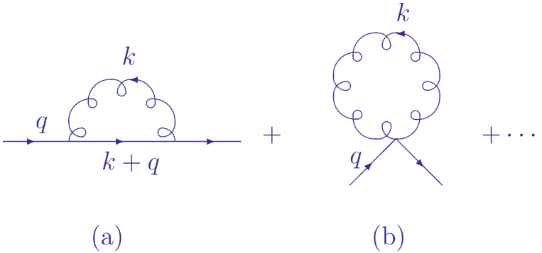
Figure 1: Graviton loop contributions to the scalar propagator. $q$ is the 4-momentum of the scalar.

We would like to take advantage of the following physical effect that is intrinsic in Einstein’s formulation of Newton’s law: for large Euclidean momenta, where the squared momentum transfer in Fig. 1 has a large negative value, the gravitational self-energy from Newton’s law is strongly repulsive, so that propagation of the particle in this regime should be severely damped in the exact solutions of the theory in (2). This is an intuitive explanation for the success of Weinberg’s asymptotic safety approach as recently realized phenomenologically in Refs. [24, 25, 26, 27] and leads us to try to resum the large parts of the quantum gravitational loop corrections in order to improve the convergence of the respective Feynman series.

We, however, do not wish to drop-out pieces of this Feynman series. We wish to make an exact re-arrangement of the series in which some of the large gravitational quantum loop effects are resummed to all orders in the loop expansion. Which large gravitational effects shall we resum? In the general Feynman one-loop integral, enhanced contributions arise from three regimes:

• the ultra-violet regime

• the collinear regime

• the infrared regime

The ultra-violet regime will be treated by the renormalization program which we seek to establish here. The collinear regime has been addressed in non-Abelian gauge theories by many authors [42] and we would expect to be able to apply the respective methods to the improved loop expansion that we seek to establish here as well. These methods are as yet generally approximate in the sense of our discussion, they are generically not exact re-arrangements of the Feynman series. We thus look to the infrared regime, for which exact re-arrangement of the loop expansion has been achieved by Yennie, Frautschi and Suura (YFS) in Ref. [18] for Abelian massless gauge theories. In Refs. [20], we have shown that the YFS methods can be extended to non-Abelian gauge theories with the understanding that only the leading IR singular terms actually exponentiate in the YFS sense and that the remaining non-leading and genuinely non-Abelian IR singular terms are treated order by order in the loop expansion. Physically, resummimg this leading IR singular part of the loop expansion in quantum general relativity offers the possibility of improving the convergence of the resummed loop expansion and curing the long standing problem of the non-renormalizability of Einstein’s theory. That is what we will argue actually happens in the following.

We note here that, already in Ref. [18], it has been pointed-out that YFS resummation of the IR effects in QED improves the UV convergence for the Feynman series for QED. This occurs for the electron propagator but not for the photon propagator and , as the coupling parameter in the soft regime is just $\alpha_{em}\cong\frac{1}{137}$, the improvement in the convergence via the electron propagator is very marginal, for it is the asymptotic behavior $\frac{1}{p^{1+{\cal O}(\alpha_{em})}}$ vs $\frac{1}{p}$ in the deep Euclidean regime. For quantum general general relativity, we will see below that all particles’ propagators are improved and that the improvement becomes pronounced in the deep Euclidean regime and causes all propagators to fall faster than any power of the respective momentum transfer $p$.

Returning to Fig. 1, we write the respective contributions to the 1PI proper 2-point vertex function, $-i\Sigma(p)$, the proper self-energy contribution to inverse propagator here, as

$$-i\left(\Delta_{F}(p)^{-1}-\Sigma(p)\right)=i\sum_{n=o}^{\infty}\Sigma_{n}(p)$$ (3)

where $-i\Sigma_{n}(p)$ is the respective n-loop contribution with the agreement that for $n=0$ we have $-\Sigma_{0}(p)=\Delta_{F}(p)^{-1}=p^{2}-m^{2}+i\epsilon$ For the latter n-loop contribution, we first represent it as follows:

$$i\Sigma_{n}(p)=\frac{1}{n!}\int\cdots\int\prod_{i=1}^{n}\frac{dk_{i}}{k_{i}^{2}-\lambda^{2}+i\epsilon}\rho_{n}(k_{1},\cdots,k_{n})$$ (4)

where the function $\rho_{n}$ is symmetric under the interchange of any two of the n virtual graviton 4-momenta that are exchanged in (4), by the Bose symmetry obeyed by the spin 2 gravitons and the symmetry of the respective multiple integration volume. Here is the point in the discussion where the power of exact rearrangement techniques such as those in Ref. [18] enters. For the case $n=1$, let $S^{\prime\prime}_{g}(k)\rho_{0}$ represent the leading contribution in the the limit $k\rightarrow 0$ to $\rho_{1}$. We have

$$\rho_{1}(k)=S^{\prime\prime}_{g}(k)\rho_{0}+\beta_{1}(k)$$ (5)

where this equation is exact and serves to define $\beta_{1}$ if we specify $S^{\prime\prime}_{g}(k)$, the soft graviton emission factor, and recall that

$$\rho_{0}=i\Sigma_{0}(p)=-i\Delta_{F}(p)^{-1}.$$ (6)

This can be determined from the Feynman rules for (2) or one can also use the off-shell extension of the formulas in Ref. [2]. We get [32]

$$\begin{split}S^{\prime\prime}_{g}(p,p,k)&=\frac{1}{(2\pi)^{4}}\frac{i\frac{1}{2}(\eta^{\mu\nu}\eta^{\bar{\mu}\bar{\nu}}+\eta^{\mu\bar{\nu}}\eta^{\bar{\mu}\nu}-\eta^{\mu\bar{\mu}}\eta^{\nu\bar{\nu}})(-i\kappa p_{\bar{\mu}})(2ip_{\mu})(-i\kappa{p^{\prime}}_{\bar{\nu}})(2i{p^{\prime}}_{\nu})}{(k^{2}-2kp+\Delta+i\epsilon)(k^{2}-2kp^{\prime}+\Delta^{\prime}+i\epsilon)}{\Big{|}}_{p=p^{\prime}}\\ &=\frac{2i\kappa^{2}p^{4}}{16\pi^{4}}\frac{1}{(k^{2}-2kp+\Delta+i\epsilon)^{2}}\end{split}$$ (7)

where $\Delta=p^{2}-m^{2}$, $\Delta^{\prime}={p^{\prime}}^{2}-m^{2}$. To see this, from Fig. 1, note that the Feynman rules give us the following result

$$\begin{split}i\Sigma_{1}(p)&=\Big{\{}-\frac{\int d^{4}k}{(2\pi)^{4}}iv_{3}(p,p-k)_{\mu\bar{\mu}}\frac{i}{(p-k)^{2}-m^{2}+i\epsilon}iv_{3}(p-k,p^{\prime})_{\nu\bar{\nu}}\\ &\qquad\qquad\frac{i\frac{1}{2}(\eta^{\mu\nu}\eta^{\bar{\mu}\bar{\nu}}+\eta^{\mu\bar{\nu}}\eta^{\bar{\mu}\nu}-\eta^{\mu\bar{\mu}}\eta^{\nu\bar{\nu}})}{k^{2}-\lambda^{2}+i\epsilon}\\ &\qquad-\frac{\int d^{4}k}{2(2\pi)^{4}}iv_{4}(p,p^{\prime})_{\mu\bar{\mu};\nu\bar{\nu}}\frac{i\frac{1}{2}(\eta^{\mu\nu}\eta^{\bar{\mu}\bar{\nu}}+\eta^{\mu\bar{\nu}}\eta^{\bar{\mu}\nu}-\eta^{\mu\bar{\mu}}\eta^{\nu\bar{\nu}})}{k^{2}-\lambda^{2}+i\epsilon}\Big{\}}\Big{|}_{p=p^{\prime}},\end{split}$$ (8)

where we have defined from the Feynman rules the respective 3-point($h\varphi\varphi$ and 4-point($hh\varphi\varphi$) vertices

$$\begin{split}iv_{3}(p,p^{\prime})_{\nu\bar{\nu}}&=-i\kappa\left(p_{\nu}{p^{\prime}}_{\bar{\nu}}+p_{\bar{\nu}}{p^{\prime}}_{\nu}-g_{\nu\bar{\nu}}(pp^{\prime}-m^{2})\right)\\ iv_{4}(p,p^{\prime})_{\mu\bar{\mu};\nu\bar{\nu}}&=-4i\kappa^{2}[(pp^{\prime}-m^{2})(\eta_{\mu\bar{\nu}}\eta_{\bar{\mu}\nu}+\eta_{\bar{\mu}\bar{\nu}}\eta_{\mu\nu}-\eta_{\mu\bar{\mu}}\eta_{\nu\bar{\nu}})\\ &\qquad\qquad-(p^{\mu^{\prime}}{p^{\prime}}^{\nu^{\prime}}+p^{\nu^{\prime}}{p^{\prime}}^{\mu^{\prime}})\{\eta_{\mu\mu^{\prime}}(\eta_{\bar{\mu}\nu}\eta_{\nu^{\prime}\bar{\nu}}+\eta_{\bar{\mu}\bar{\nu}}\eta_{\nu^{\prime}\nu}-\eta_{\nu^{\prime}\bar{\mu}}\eta_{\nu\bar{\nu}})\\ &\qquad\qquad+\eta_{\bar{\mu}\mu^{\prime}}(\eta_{\mu\nu}\eta_{\nu^{\prime}\bar{\nu}}+\eta_{\mu\bar{\nu}}\eta_{\nu^{\prime}\nu}-\eta_{\nu^{\prime}\mu}\eta_{\nu\bar{\nu}})\}]\end{split}$$ (9)

using the standard conventions so that p is incoming and p’ is outgoing for the scalar particle momenta at the respective vertices. In this way, we see that we may isolate the IR dominant part of $i\Sigma_{1}(p)$ by the separation

$$\begin{split}\frac{1}{k^{2}-2kp+\Delta+i\epsilon}&=-\frac{\Delta}{(k^{2}-2kp+\Delta+i\epsilon)^{2}}+\frac{1}{k^{2}-2kp+i\epsilon}\\ &\qquad-\frac{2\Delta^{2}}{(k^{2}-2kp+\Delta+i\epsilon)^{2}(k^{2}-2kp+i\epsilon)}\\ &\qquad-\frac{\Delta^{3}}{(k^{2}-2kp+\Delta+i\epsilon)^{2}(k^{2}-2kp+i\epsilon)^{2}}\\ &\qquad+\sum_{n=2}^{\infty}(-1)^{n}\frac{\Delta^{n}}{(k^{2}-2kp+i\epsilon)^{n+1}}\end{split}$$ (10)

from which we can see that the first term on the RHS gives, upon insertion into (8), the IR-divergent contribution for the coefficient of the lowest order inverse propagator for the on-shell limit $\Delta\rightarrow 0$. The second term does not produce an IR-divergence and the remaining terms vanish faster than $\Delta$ in the on-shell limit so that they do not contribute to the field renormalization factor which we seek to isolate. In this way we get finally

$$\begin{split}i\Sigma_{1}(p)&=\Big{\{}-\frac{\int d^{4}k}{(2\pi)^{4}}(-2i\kappa p_{\mu}p_{\bar{\mu}}+i\delta{v_{3}(p,p-k)_{\mu\bar{\mu}}})(\frac{-i\Delta}{(k^{2}-2kp+\Delta+i\epsilon)^{2}}+i~{}R\Delta_{F}(k,p))\\ &\qquad\qquad(-2i\kappa{p}^{\prime}_{\nu}{p^{\prime}}_{\bar{\nu}}+i\delta{v_{3}(p^{\prime}-k,p^{\prime})_{\nu\bar{\nu}}})\frac{i\frac{1}{2}(\eta^{\mu\nu}\eta^{\bar{\mu}\bar{\nu}}+\eta^{\mu\bar{\nu}}\eta^{\bar{\mu}\nu}-\eta^{\mu\bar{\mu}}\eta^{\nu\bar{\nu}})}{k^{2}-\lambda^{2}+i\epsilon}\\ &\qquad-\frac{\int d^{4}k}{2(2\pi)^{4}}iv_{4}(p,p^{\prime})_{\mu\bar{\mu};\nu\bar{\nu}}\frac{i\frac{1}{2}(\eta^{\mu\nu}\eta^{\bar{\mu}\bar{\nu}}+\eta^{\mu\bar{\nu}}\eta^{\bar{\mu}\nu}-\eta^{\mu\bar{\mu}}\eta^{\nu\bar{\nu}})}{k^{2}-\lambda^{2}+i\epsilon}\Big{\}}\Big{|}_{p=p^{\prime}}\\ &\qquad=\Big{\{}\frac{\int d^{4}k}{(2\pi)^{4}}[(-i\kappa p_{\bar{\mu}})(2ip_{\mu})\frac{-i\Delta}{(k^{2}-2kp+\Delta+i\epsilon)^{2}}(-i\kappa{p^{\prime}}_{\bar{\nu}})(2i{p^{\prime}}_{\nu})\\ &\qquad\qquad\frac{i\frac{1}{2}(\eta^{\mu\nu}\eta^{\bar{\mu}\bar{\nu}}+\eta^{\mu\bar{\nu}}\eta^{\bar{\mu}\nu}-\eta^{\mu\bar{\mu}}\eta^{\nu\bar{\nu}})}{k^{2}-\lambda^{2}+i\epsilon}+\frac{(2\pi)^{4}\beta_{1}(k)}{k^{2}-\lambda^{2}+i\epsilon}]\Big{\}}\Big{|}_{p=p^{\prime}},\end{split}$$ (11)

which agrees with (5,6,7) with

$$\begin{split}R\Delta_{F}(k,p)&=\frac{1}{k^{2}-2kp+i\epsilon}-\frac{2\Delta^{2}}{(k^{2}-2kp+\Delta+i\epsilon)^{2}(k^{2}-2kp+i\epsilon)}\\ &\qquad-\frac{\Delta^{3}}{(k^{2}-2kp+\Delta+i\epsilon)^{2}(k^{2}-2kp+i\epsilon)^{2}}\\ &\qquad+\sum_{n=2}^{\infty}(-1)^{n}\frac{\Delta^{n}}{(k^{2}-2kp+i\epsilon)^{n+1}},\\ i\delta{v_{3}(p,p-k)_{\mu\bar{\mu}}}&=iv_{3}(p,p-k)_{\mu\bar{\mu}}-\{-2i\kappa p_{\mu}p_{\bar{\mu}}\},\\ \beta_{1}(k)&=\Big{\{}-\frac{1}{(2\pi)^{4}}(-2i\kappa p_{\mu}p_{\bar{\mu}}+i\delta{v_{3}(p,p-k)_{\mu\bar{\mu}}})[\frac{-i\Delta}{(k^{2}-2kp+\Delta+i\epsilon)^{2}}\\ &\qquad\qquad+i~{}R\Delta_{F}(k,p)](i\delta{v_{3}(p^{\prime}-k,p^{\prime})_{\nu\bar{\nu}}})\{i\frac{1}{2}(\eta^{\mu\nu}\eta^{\bar{\mu}\bar{\nu}}+\eta^{\mu\bar{\nu}}\eta^{\bar{\mu}\nu}-\eta^{\mu\bar{\mu}}\eta^{\nu\bar{\nu}})\}\\ &\qquad\qquad-\frac{1}{(2\pi)^{4}}(-2i\kappa p_{\mu}p_{\bar{\mu}}+i\delta{v_{3}(p,p-k)_{\mu\bar{\mu}}})(i~{}R\Delta_{F}(k,p))\\ &\qquad\qquad(-2i\kappa{p}^{\prime}_{\nu}{p^{\prime}}_{\bar{\nu}})\{i\frac{1}{2}(\eta^{\mu\nu}\eta^{\bar{\mu}\bar{\nu}}+\eta^{\mu\bar{\nu}}\eta^{\bar{\mu}\nu}-\eta^{\mu\bar{\mu}}\eta^{\nu\bar{\nu}})\}\\ &\qquad\qquad-\frac{1}{(2\pi)^{4}}(i\delta{v_{3}(p,p-k)_{\mu\bar{\mu}}})(\frac{-i\Delta}{(k^{2}-2kp+\Delta+i\epsilon)^{2}})\\ &\qquad\qquad(-2i\kappa{p}^{\prime}_{\nu}{p^{\prime}}_{\bar{\nu}})\{i\frac{1}{2}(\eta^{\mu\nu}\eta^{\bar{\mu}\bar{\nu}}+\eta^{\mu\bar{\nu}}\eta^{\bar{\mu}\nu}-\eta^{\mu\bar{\mu}}\eta^{\nu\bar{\nu}})\}\\ &\qquad\qquad-\frac{1}{2(2\pi)^{4}}iv_{4}(p,p^{\prime})_{\mu\bar{\mu};\nu\bar{\nu}}\{i\frac{1}{2}(\eta^{\mu\nu}\eta^{\bar{\mu}\bar{\nu}}+\eta^{\mu\bar{\nu}}\eta^{\bar{\mu}\nu}-\eta^{\mu\bar{\mu}}\eta^{\nu\bar{\nu}})\}\Big{\}}\Big{|}_{p=p^{\prime}}.\end{split}$$ (12)

One can see that the result in (7) differs from the corresponding result in QED in eq.(5.13) of Ref. [18] by the replacement of the electron charges $e$ by the gravity charges $\kappa p_{\bar{\mu}},~{}\kappa{p^{\prime}}_{\bar{\nu}}$ with the corresponding replacement of the photon propagator numerator $-i\eta_{\mu\nu}$ by the graviton propagator numerator $i\frac{1}{2}(\eta^{\mu\nu}\eta^{\bar{\mu}\bar{\nu}}+\eta^{\mu\bar{\nu}}\eta^{\bar{\mu}\nu}-\eta^{\mu\bar{\mu}}\eta^{\nu\bar{\nu}})$. That the squared modulus of these gravity charges grows quadratically in the deep Euclidean regime is what makes their effect therein in the quantum theory of general relativity fundamentally different from the effect of the QED charges in the deep Euclidean regime of QED, where the latter charges are constants order-by-order in perturbation theory.

Indeed, proceeding recursively, we write

$$\rho_{n}(k_{1},\cdots,k_{n})=S^{\prime\prime}_{g}(k_{n})\rho_{n-1}(k_{1},\cdots,k_{n-1})+\beta^{(1)}_{n}(k_{1},\cdots,k_{n-1};k_{n})$$ (13)

where here the notation indicates that the residual $\beta^{(1)}_{n}$ does not contain the leading infrared contribution for $k_{n}$ that is given by the first term on the RHS of (13). We iterate (13) to get

$$\begin{split}\rho_{n}(k_{1},\cdots,k_{n})&=S^{\prime\prime}_{g}(k_{n})S^{\prime\prime}_{g}(k_{n-1})\rho_{n-2}(k_{1},\cdots,k_{n-2})\\ &+S^{\prime\prime}_{g}(k_{n})\beta^{(1)}_{n-1}(k_{1},\cdots,k_{n-2};k_{n-1})\\ &+S^{\prime\prime}_{g}(k_{n-1})\beta^{(1)}_{n-1}(k_{1},\cdots,k_{n-2};k_{n})\\ &+\{-S^{\prime\prime}_{g}(k_{n-1})\beta^{(1)}_{n-1}(k_{1},\cdots,k_{n-2};k_{n})+\beta^{(1)}_{n}(k_{1},\cdots,k_{n-1};k_{n})\}\end{split}$$ (14)

The symmetry of $\rho_{n}$ implies that the quantity in curly brackets is also symmetric in the interchange of $k_{n-1}$ and $k_{n}$. We indicate this explicitly with the notation

$$\{-S^{\prime\prime}_{g}(k_{n-1})\beta^{(1)}_{n-1}(k_{1},\cdots,k_{n-2};k_{n})+\beta^{(1)}_{n}(k_{1},\cdots,k_{n-1};k_{n})\}=\beta^{(2)}_{n}(k_{1},\cdots,k_{n-2};k_{n-1},k_{n}).$$ (15)

Repeated application of (13) and use of the symmetry of $\rho_{n}$ leads us finally to the exact result

$$\begin{split}\rho_{n}(k_{1},\cdots,k_{n})&=S^{\prime\prime}_{g}(k_{1})\cdots S^{\prime\prime}_{g}(k_{n})\beta_{0}\\ &+\sum_{i=1}^{n}S^{\prime\prime}_{g}(k_{1})\cdots S^{\prime\prime}_{g}(k_{i-1})S^{\prime\prime}_{g}(k_{i+1})\cdots S^{\prime\prime}_{g}(k_{n})\beta_{1}(k_{i})\\ &+\cdots+\sum_{i=1}^{n}S^{\prime\prime}_{g}(k_{i})\beta_{n-1}(k_{1},\cdots,k_{i-1},k_{i+1},\cdots,k_{n})+\beta_{n}(k_{1},\cdots,k_{n})\end{split}$$ (16)

where the case n=1 has already been considered in (5) with $\rho_{0}\equiv\beta_{0}$. Here, we defined as well $\beta^{(i)}_{i}\equiv\beta_{i}$.

We can use the symmetry of the residuals $\beta_{i}$ to re-write $\rho_{n}$ as

$$\rho_{n}(k_{1},\cdots,k_{n})=\sum_{perm}\sum_{r=0}^{n}\frac{1}{r!(n-r)!}\prod_{i=1}^{r}S^{\prime\prime}_{g}(k_{i})\beta_{n-r}(k_{r+1},\cdots,k_{n})$$ (17)

so that we finally obtain, upon substitution into (4),

$$i\Sigma_{n}(p)=\sum_{r=0}^{n}\frac{1}{r!(n-r)!}\left(\int\frac{d^{4}k~{}S^{\prime\prime}_{g}(k)}{k^{2}-\lambda^{2}+i\epsilon}\right)^{r}\int\prod_{i=1}^{n-r}\frac{d^{4}k_{i}}{{k_{i}}^{2}-\lambda^{2}+i\epsilon}\beta_{n-r}(k_{1},\cdots,k_{n-r}).$$ (18)

With the definition

$$-B^{\prime\prime}_{g}(p)=\int\frac{d^{4}k~{}S^{\prime\prime}_{g}(k)}{k^{2}-\lambda^{2}+i\epsilon}$$ (19)

and the identification

$$i\Sigma^{\prime}_{r}(p)=\frac{1}{r!}\int\prod_{i=1}^{r}\frac{d^{4}k_{i}}{k_{i}^{2}-\lambda^{2}+i\epsilon}\beta_{r}(k_{1},\cdots,k_{r})$$ (20)

we introduce the result (18) into (3) to get

$$\begin{split}-i\left(\Delta_{F}(p)^{-1}-\Sigma(p)\right)&=i\sum_{n=0}^{\infty}\sum_{r=0}^{n}\Sigma^{\prime}_{n-r}(p)\frac{(-B^{\prime\prime}_{g}(p))^{r}}{r!}\\ &=ie^{-B^{\prime\prime}_{g}(p)}\sum_{\ell=0}^{\infty}\Sigma^{\prime}_{\ell}(p)\\ &=-ie^{-B^{\prime\prime}_{g}(p)}\left(\Delta_{F}(p)^{-1}-\sum_{\ell=1}^{\infty}\Sigma^{\prime}_{\ell}(p)\right).\end{split}$$ (21)

In this way, our resummed exact result for the complete propagator in quantum general relativity is seen to be [32, 33, 34]

$$i\Delta^{\prime}_{F}(p)|_{\text{resummed}}=\frac{ie^{B^{\prime\prime}_{g}(p)}}{(p^{2}-m^{2}-\Sigma^{\prime}_{s}(p)+i\epsilon)}$$ (22)

where

$$\Sigma^{\prime}_{s}(p)\equiv\sum_{\ell=1}^{\infty}\Sigma^{\prime}_{\ell}(p).$$ (23)

Some observations are in order before we turn to the consequences of (22). First, we have not modified Einstein’s theory at all. This means we are developing a very conservative approach to treat the UV behavior of of quantum general relativity. This makes our approach interesting in its own right, as we have noted in the Introduction. Second, because we did not modify the theory, what we have done is necessarily gauge invariant, as the original theory was gauge invariant. Third, the IR-improved $\Sigma^{\prime}_{s}(p)$ is already organized in a loop expansion by our derivation of (23). We expect therefore to be able to treat it perturbatively when the physics allows us to so do.

To see the effect of the exponential factor in (22), we evaluate the exponent as follows for Euclidean momenta ( see Appendix 1 for the details of the attendant evaluation )

$$B^{\prime\prime}_{g}(k)=\frac{\kappa^{2}|k^{2}|}{8\pi^{2}}\ln\left(\frac{m^{2}}{m^{2}+|k^{2}|}\right).$$ (24)

The latter result establishes the advertised behavior: in the deep Euclidean regime, the resummed propagator falls faster than any finite power of $|k^{2}|$. This is exactly the type of behavior we need to tame the bad UV behavior of quantum general relativity.

We have in fact shown in Ref. [32] that the exponentially damped behavior in the the propagator in (22), which holds for all particles because gravity couples in the infrared universally to all particles, leads to the UV finiteness of quantum general relativity, which is completely consistent with asymptotic safety [22]. The proof is given explicitly in Ref. [32] – see especially pages 6-8 of the latter reference – for completeness, we record it in Appendix 3 here. In the next section, we turn to some of the further consequences of the improved propagator behavior and UV finiteness we have found in our new approach to quantum general relativity.

4 Resummed Quantum Gravity and Newton’s Law: Some Consequences

An immediate consequence of our new UV finite quantum loop results for QGR is that we can make exact, UV finite, predictions for the quantum loop corrections [32, 33, 34, 35] to Newton’s law. These results are then unique because we do not modify Einstein’s theory or quantum mechanics to obtain them and we have no free parameters. We now present our prediction for the quantum loop corrections to Newton’s law in this Section.

Specifically, consider the diagrams in Figs. 2 and 3. These graphs have a superficial degree of divergence in the UV of +4 and in the usual treatment of the theory they are well-known to generate a UV divergence in the respective 1PI 2-point function for the coefficient of $q^{4}$, a divergence that thus can not be removed by the standard field and mass renormalizations. Any successful treatment of the UV behavior of QGR must therefore render this divergence finite. Indeed, when the graphs Figs. 2 and 3 are computed in our resummed quantum gravity

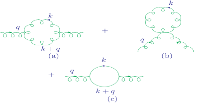
Figure 2: The graviton((a),(b)) and its ghost((c)) one-loop contributions to the graviton propagator. $q$ is the 4-momentum of the graviton.

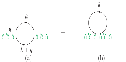
Figure 3: The scalar one-loop contribution to the graviton propagator. $q$ is the 4-momentum of the graviton.

theory, this is precisely what happens.

For example, consider the graph in Fig. 3a. When we use our resummed propagators, we get (here, $k\rightarrow(ik^{0},\vec{k})$ by Wick rotation, and we work in the transverse-traceless space)

$$\begin{split}i\Sigma(q)^{1a}_{\bar{\mu}\bar{\nu};\mu\nu}&=i\kappa^{2}\frac{\int d^{4}k}{2(2\pi)^{4}}\frac{\left(k^{\prime}_{\bar{\mu}}k_{\bar{\nu}}+k^{\prime}_{\bar{\nu}}k_{\bar{\mu}}\right)e^{\frac{\kappa^{2}|{k^{\prime}}^{2}|}{8\pi^{2}}\ln\left(\frac{m^{2}}{m^{2}+|{k^{\prime}}^{2}|}\right)}}{\left({k^{\prime}}^{2}-m^{2}+i\epsilon\right)}\\ &\qquad\frac{\left(k^{\prime}_{\mu}k_{\nu}+k^{\prime}_{\nu}k_{\mu}\right)e^{\frac{\kappa^{2}|k^{2}|}{8\pi^{2}}\ln\left(\frac{m^{2}}{m^{2}+|k^{2}|}\right)}}{\left(k^{2}-m^{2}+i\epsilon\right)}.\end{split}$$ (25)

We see explicitly that the exponential damping in the deep Euclidean regime has rendered the graph in Fig. 3a finite in the UV. Similarly are all the graphs in Figs. 2 and 3 UV finite when we use our respective resummed propagators to compute them.

To evaluate the effect of the corrections in Figs. 2 and 3 on the graviton propagator, we continue to work in the transverse, traceless space and isolate the effects from Figs. 2 and 3 on the coefficient of the $q^{4}$ in the graviton propagator denominator,

$$q^{2}+\frac{1}{2}q^{4}\Sigma^{T(2)}+i\epsilon,$$ (26)

so that we need to evaluate the transverse, traceless self-energy function $\Sigma^{T}(q^{2})$ that follows from eq.(25) for Fig. 3a and its analogs for Figs. 3b and 2 by the standard methods. Here, we work in the expectation that, in consequence to the newly UV finite calculated quantum loop effects in Figs. 2 and 3, the Fourier transform of the graviton propagator that enters Newton’s law, our ultimate goal here, will receive support from from $|q|^{2}<<M_{Pl}^{2}$. We will therefore work in the limit that $q^{2}/M_{Pl}^{2}$ is relatively small, $\lesssim.1$, for example. This will allow us to see the dominant effects of our new finite quantum loop effects. In other words, we will work to $\sim 10\%$ accuracy in what follows.

First let us dispense with the contributions from Figs. 2b and Fig. 3b. These are independent of $q^{2}$ so that we use a mass counter-term to remove them and set the graviton mass to $0$. Following the suggestion of Feynman in Ref. [12], we will change this to a small non-zero value below to take into account the recently established small value of the cosmological constant [39]. See also the discussion in Ref. [40] where it is shown that the quantum fluctuations in the exact de Sitter metric implied by the non-zero cosmological constant correspond in general to a mass for the graviton. Here, as we expand about a flat background, we take this effect into account as a small infrared regulator for the graviton. The deviations from flat space in the deep Euclidean region that we study due to the observed value of the cosmological constant are at the level of $e^{10^{-61}}-1$! This is safely well beyond the accuracy of our methods.

Returning to Fig. 3a, when we project onto the transverse, traceless space, that is to say, the graviton helicity space $\{e^{\mu\nu}(\pm 2)=\epsilon^{\mu}_{\pm}\epsilon^{\nu}_{\pm},\,\text{where}\,\epsilon^{\nu}_{\pm}=\pm(\hat{x}\pm i\hat{y})/\sqrt{2}\,\text{when}\,\\ \hat{x},~{}\hat{y}\,\text{are purely space-like and}(\vec{\hat{x}},\vec{\hat{y}},\vec{q}/|\vec{q}|)\,\text{form a right-handed coordinate basis}\}$, we get (see the Appendix 2) the result

$$i\Sigma^{T}(q^{2})_{3a}=\frac{-i\kappa^{2}m^{4}}{96\pi^{2}}\int^{1}_{0}d\alpha\int^{\infty}_{0}dx\frac{x^{3}(2(x+1)\bar{d}+\bar{d}^{2})}{(x+1)^{2}(x+1+\bar{d})^{2}}(1+x)^{-\lambda_{c}x}$$ (27)

where $\lambda_{c}=\frac{2m^{2}}{\pi M_{Pl}^{2}}$, $\bar{d}=\alpha(1-\alpha)\vec{q}^{2}/m^{2}$ so that we have made the substitution $x=k^{2}$ and imposed the mass counter-term as we noted. We have taken for definiteness $q=(0,\vec{q})$. We also use $q=|\vec{q}|$ when there is no chance for confusion. We are evaluating (27) in the deep UV where $m^{2}/q^{2}<<1$ and where $q^{2}/M_{Pl}^{2}\lesssim 0.1$. In this case, we get

$$i\Sigma^{T}(q^{2})_{3a}=\frac{-i\kappa^{2}}{96\pi^{2}}\left(\frac{|\vec{q}|^{2}m^{2}c_{1}}{3}+\frac{|\vec{q}|^{4}c_{2}}{30}\right)$$ (28)

where

$$\begin{split}c_{1}=I_{1}(\lambda_{c})&=\int^{\infty}_{0}dxx^{3}(1+x)^{-3-\lambda_{c}x}\\ c_{2}=I_{2}(\lambda_{c})&=\int^{\infty}_{0}dxx^{3}(1+x)^{-4-\lambda_{c}x}.\end{split}$$ (29)

Using the usual field renormalization, we see that Fig. 3a makes the contribution

$$i\tilde{\Sigma}^{T}(q^{2})_{3a}\cong\frac{-i\kappa^{2}|\vec{q}|^{4}c_{2}}{2880\pi^{2}}$$ (30)

to the transverse traceless graviton proper self-energy function.

Turning now to Figs. 2, the pure gravity loops, we use a contact between our work and that of Refs. [43]. In Refs. [43], the entire set of one-loop divergences have been computed for the theory in (2). The basic observation is the following. As we work only to the leading logarithmic accuracy in $\ln\lambda_{c}$, it is sufficient to identify the correspondence between the divergences as calculated in the n-dimensional regularization scheme in Ref. [43] and as they would occur when $\lambda_{c}\rightarrow 0$. This we do by comparing our result for (27) when $q^{2}\rightarrow 0$ with the corresponding result in Ref. [43] for the same theory. In this way we see that we have the correspondence

$$-\ln\lambda_{c}\leftrightarrow\frac{1}{2-n/2}.$$ (31)

This allows us to read-off the leading log result for the pure gravity loops directly from the results in Ref. [43]. Since $-\ln\lambda_{c}=\ln{M_{Pl}}^{2}-\ln m^{2}-\ln\frac{2}{\pi}$, we see that our exponentiated propagators have cut-off our UV divergences at the scale $\sim M_{Pl}$ and the correspondence in (31) shows the usual relation between the effective UV cut-off scale and the pole in $(2-n/2)$ in dimensional regularization.

Specifically, the result in Ref. [43], when interpreted as we have just explained, is that the pure gravity loops give a factor of 42 times the scalar loops for the coefficient $a_{2}$ above when we work in the regime where $|q^{2}|$ is relatively small compared to $M_{Pl}^{2}$. Here, we also take into account the recent significant evidence for a non-zero cosmological constant [39], which can be seen to provide a small non-zero rest mass for the graviton, $m_{g}\cong 3.1\times 10^{-33}$eV, which serves as an IR regulator for the graviton. This is the value of rest mass in $\lambda_{c}$ which should be used for pure gravitational loops. See the Appendix 1 for the derivation of the corresponding infrared exponents.

We note that, for $\lambda_{c}=0$, the constant $c_{2}$ is infinite and, as we have already imposed both the mass and field renormalization counter-terms, there would be no physical parameter into which that infinity could be absorbed: this is just another manifestation that QGR, without our resummation, is a non-renormalizable theory.

Using the universality of the coupling of the graviton when the momentum transfer scale is relatively small compared to $M_{Pl}$, we can extend the result for the scalar field above to the remaining known particles in the Standard Model by counting the number of physical degrees of freedom for each such particle and replacing the mass of the scalar with the respective mass of that particle. For a massive fermion we get a factor of 4 relative to the scalar result with the appropriate change in the mass parameter from $m$ to $m_{f}$, the mass of that fermion, for a massive vector, we get a factor of 3 relative to the scalar result, with the corresponding change in the mass from $m$ to $m_{V}$, the mass of that vector, etc. In this way, we arrive at the result that the denominator of the graviton propagator becomes, in the Standard Model,

$$q^{2}+\Sigma^{T}(q^{2})+i\epsilon\cong q^{2}-q^{4}\frac{c_{2,eff}}{360\pi M_{Pl}^{2}},$$ (32)

where we have defined

$$\begin{split}c_{2,eff}&=\sum_{\text{SM particles j}}n_{j}I_{2}(\lambda_{c}(j))\\ &\cong 2.56\times 10^{4}\end{split}$$ (33)

with $I_{2}$ defined above and with $\lambda_{c}(j)=\frac{2m_{j}^{2}}{\pi M_{Pl}^{2}}$ and [34] $n_{j}$ equal to the number of effective degrees of particle $j$ as already illustrated. In arriving at (33), we take the SM masses as follows: for the now presumed three massive neutrinos [44], we estimate a mass at $\sim 3$ eV; for the remaining members of the known three generations of Dirac fermions $\{e,\mu,\tau,u,d,s,c,b,t\}$, we use [45, 46] $m_{e}\cong 0.51$ MeV, $m_{\mu}\cong 0.106$ GeV, $m_{\tau}\cong 1.78$ GeV, $m_{u}\cong 5.1$ MeV, $m_{d}\cong 8.9$ MeV, $m_{s}\cong 0.17$ GeV, $m_{c}\cong 1.3$ GeV, $m_{b}\cong 4.5$ GeV and $m_{t}\cong 174$ GeV and for the massive vector bosons $W^{\pm},~{}Z$ we use the masses $M_{W}\cong 80.4$ GeV, $M_{Z}\cong 91.19$ GeV, respectively. We note that (see the Appendix 1) when the rest mass of particle $j$ is zero, the value of $m_{j}$ turns-out to be $\sqrt{2}$ times the gravitational infrared cut-off mass [39], which is $m_{g}\cong 3.1\times 10^{-33}$eV. We further note that, from the exact one-loop analysis of Ref.[43], it also follows that the value of $n_{j}$ for the graviton and its attendant ghost is $42$. For $\lambda_{c}\rightarrow 0$, we have found the approximate representation

$$I_{2}(\lambda_{c})\cong\ln\frac{1}{\lambda_{c}}-\ln\ln\frac{1}{\lambda_{c}}-\frac{\ln\ln\frac{1}{\lambda_{c}}}{\ln\frac{1}{\lambda_{c}}-\ln\ln\frac{1}{\lambda_{c}}}-\frac{11}{6}.$$ (34)

If we use the standard Fourier transform of the respective graviton propagator we obtain the improved Newton potential

$$\Phi_{N}(r)=-\frac{G_{N}M}{r}(1-e^{-ar}),$$ (35)

where with

$$a\cong(\frac{360\pi M_{Pl}^{2}}{c_{2,eff}})^{\frac{1}{2}}$$ (36)

we have that

$$a\cong 0.210M_{Pl}.$$ (37)

We note that the implied behavior of the running Newton constant, $G_{N}(k)$, that corresponds to our resummed graviton propagator denominator,

$$G_{N}(k)=\frac{G_{N}}{1+k^{2}/a^{2}},$$ (38)

agrees with the large (Euclidean) $k^{2}$ limit of $G_{N}(k)$ found by the authors in Ref. [25] using the asymptotic safety approach as realized by phenomenological exact renormalization group methods – we agree as well on the generic size of $a$. The connection between k and position space in our analysis is given by the usual Fourier transformation method whereas that in Ref. [25] involves a phenomenological parameter which is ideally determined self-consistently. Thus, as we will see below, while our results and the results in Ref. [25] agree on $G_{N}(k)$ for large values of $k$, our forms for the corresponding Newton potential differ in position space: we expect our result to hold in the deep Euclidean regime whereas at larger distances the result in Ref. [25] should be preferred.

We also note that the behavior of the graviton propagator found by our analysis and by that in Ref. [25] agrees for large Euclidean $k^{2}$ with that in the $R^{2}-$quantum gravity theory [47]. However, unlike the latter theory, in our work unitarity has not been lost, as we quantize the theory using the methods of Refs. [11, 12, 4].

We discuss now two consequences of the improved Newton potential:

4.1 Elementary Particles and Black Holes

One of the issues that confronts the theory of point particle fields is that fact that a massive point particle of rest mass $m$ has its mass entirely inside of its Schwarzschild radius $r_{S}=2m/M_{Pl}^{2}$ so that classically it should be a black hole. We expect this conclusion to be modified by quantum mechanics, where the mass of such a particle seems readily accessible in experiments. Note that we distinguish here the uncertainty in the position of the particle, which is connected to its Compton wavelength when the particle is at rest, from the accessibility of the mass of that particle, which is connected to its black hole character. The situation can be addressed by focusing on the lapse function in the metric class

$$ds^{2}=f(r)dt^{2}-f(r)^{-1}dr^{2}-r^{2}d\Omega^{2},$$ (39)

with

$$f(r)=1-\frac{2G(r)m}{r}$$ (40)

and $G(r)$, using (35), given by

$$G(r)=G_{N}(1-e^{-ar}).$$ (41)

We see that the Standard Model massive particles all have the property that $f(r)$ remains positive as $r$ passes through their respective Schwarzschild radii and goes to $r=0$, so that the particle is no longer [33, 34] a black hole as it was classically. Refs. [25, 48] have also found that sub-Planck mass black holes do not exist in quantum field theory.

4.2 Final State of Hawking Radiation – Planck Scale Cosmic Rays

The situation that then naturally comes to mind is the evaporation of massive black holes. In Ref. [25], following Weinberg’s [22] asymptotic safety approach as realized by phenomenological exact renormalization group methods, it has been shown that the attendant running of Newton’s constant leads to the lapse function representation, in the metric class in (39)

$$f(r)=1-\frac{2G(r)M}{r}$$ (42)

where $M$ is the mass of the black hole and now

$$G(r)\equiv G_{BR}(r)=\frac{G_{N}r^{3}}{r^{3}+\tilde{\omega}G_{N}\left[r+\gamma G_{N}M\right]}$$ (43)

where $\gamma$ is a phenomenological parameter [25] satisfying $0\leq\gamma\leq\frac{9}{2}$ and $\tilde{\omega}=\frac{118}{15\pi}$. It can be shown that (43) leads as well to the conclusion that black holes with mass less than a critical mass $M_{cr}\sim M_{Pl}$ have no horizon, as we have argued for massive SM elementary particles. When we join our result in (40) onto that in (43) at the outermost solution, $r_{>}$, of the equation

$$G_{BR}(r)=G_{N}(1-e^{-ar}),$$ (44)

we have a result for the final state of the Hawking process for an originally very massive black hole: for $r<r_{>}$, in the lapse function we use our result in (40) for $G(r)$ and for $r>r_{>}$ we use $G_{BR}(r)$ for $G(r)$ after the originally massive black hole has Hawking radiated down to the appropriate scale. For example, for the self-consistent value $\gamma=0$ and $0.2=\Omega\equiv\frac{\tilde{\omega}}{G_{N}M^{2}}=\frac{\tilde{\omega}M_{Pl}^{2}}{M^{2}}$ for definiteness we find [35] that the inner horizon found in Ref. [25] moves to negative values of $r$ and that the outer horizon moves to $r=0$, so that the entire mass of the originally very massive black hole radiates away until a Planck scale remnant of mass $M_{cr}^{\prime}=2.38~{}M_{Pl}$ is left [25, 50] , which then is completely accessible to our universe. It would be expected to decay into n-body final states, $n=2,3,\cdots$, leading in general to Planck scale cosmic rays [34, 35]. The data in Ref. [51, 52] are not inconsistent with this conclusion, which also agrees with recent results by Hawking [53].

5 Conclusions

In this paper we have introduced a new paradigm in the history of point particle field theory: a UV finite theory of the quantum general relativity. It appears to be a solution to most of the outstanding problems in the union of the ideas of Bohr and Einstein. More importantly, it shows that quantum mechanics, while not necessarily the ultimate theory, is not an incomplete theory.

Our paradigm does not contradict any known experimental or theoretical fact; rather, it allows us to better understand the known physics and, hopefully, to make new testable predictions. Our paradigm does not contradict string theory or loop quantum gravity, to the best of our knowledge. In principle, all three approaches to quantum general relativity should agree in the appropriate regimes, where we would stress that, unlike what is suggested by the other two approaches, sub-Planck scale phenomena do exist in our approach. Further work on establishing the precise relationship between the three approaches is in progress.

Evidently, formulations for supergravity theories in Refs. [23, 54] which were abandoned as complete theories of quantum gravity because they proved to be non-renormalizable are now, with the resummation methods of this paper, rendered UV finite and thus are again phenomenologically interesting in their own right rather than as low energy approximations to surperstring theory. Of course, they may still have other problems. We will pursue this line of phenomenology elsewhere.

Appendix 1: Evaluation of Gravitational Infrared Exponent

In the text, we use several limits of the gravitational infrared exponent $B^{\prime\prime}_{g}$ defined in (19). Here, we present these evaluations for completeness.

We have to consider

$$\begin{split}-B^{\prime\prime}_{g}(p)&=\int\frac{d^{4}k~{}S^{\prime\prime}_{g}(k)}{k^{2}-\lambda^{2}+i\epsilon}\\ &=\int\frac{d^{4}k}{(2\pi)^{4}(k^{2}-\lambda^{2}+i\epsilon)}\frac{i\frac{1}{2}(\eta^{\mu\nu}\eta^{\bar{\mu}\bar{\nu}}+\eta^{\mu\bar{\nu}}\eta^{\bar{\mu}\nu}-\eta^{\mu\bar{\mu}}\eta^{\nu\bar{\nu}})(-i\kappa p_{\bar{\mu}})(2ip_{\mu})(-i\kappa{p^{\prime}}_{\bar{\nu}})(2i{p^{\prime}}_{\nu})}{(k^{2}-2kp+\Delta+i\epsilon)(k^{2}-2kp^{\prime}+\Delta^{\prime}+i\epsilon)}{\Big{|}}_{p=p^{\prime}}\\ &=\frac{2i\kappa^{2}p^{4}}{16\pi^{4}}\int\frac{d^{4}k}{(k^{2}-\lambda^{2}+i\epsilon)}\frac{1}{(k^{2}-2kp+\Delta+i\epsilon)^{2}}\end{split}$$ (45)

where $\Delta=p^{2}-m^{2}$. The integral on the RHS of (45) is given by

$$\begin{split}I&=\int\frac{d^{4}k}{(k^{2}-\lambda^{2}+i\epsilon)}\frac{1}{(k^{2}-2kp+\Delta+i\epsilon)^{2}}\\ &=\frac{-i\pi^{2}}{p^{2}}\frac{1}{x_{+}-x_{-}}{\big{[}}x_{+}\ln(1-1/(\sqrt{2}x_{+}))-x_{-}\ln(1-1/(\sqrt{2}x_{-})){\big{]}}\end{split}$$

with

$$x_{\pm}=\frac{1}{2\sqrt{2}}\left(\bar{\Delta}+\bar{\lambda}^{2}\pm((\bar{\Delta}+\bar{\lambda}^{2})^{2}-4(\bar{\lambda}^{2}-i\bar{\epsilon}))^{\small 1/2}\right)$$ (46)

for $\bar{\Delta}=1-m^{2}/p^{2},~{}\bar{\lambda}^{2}=\lambda^{2}/p^{2}\text{and}~{}\bar{\epsilon}=\epsilon/p^{2}$. In this way, we arrive at the results, for $p^{2}<0$,

$$B^{\prime\prime}_{g}(p)=\begin{cases}&\frac{\kappa^{2}|p^{2}|}{8\pi^{2}}\ln\left(\frac{m^{2}}{m^{2}+|p^{2}|}\right),~{}~{}m\neq 0\\ &\frac{\kappa^{2}|p^{2}|}{8\pi^{2}}\ln\left(\frac{m_{g}^{2}}{m_{g}^{2}+|p^{2}|}\right),~{}~{}m=m_{g}=\lambda\\ &\frac{2\kappa^{2}|p^{2}|}{8\pi^{2}}\ln\left(\frac{m_{g}^{2}}{|p^{2}|}\right),~{}~{}m=0,~{}m_{g}=\lambda\end{cases}$$ (47)

where we have made more explicit the presence of the observed small mass, $m_{g}$, of the graviton.

Appendix 2: Evaluation of Gravitationally Regulated Loop Integrals

In this section we present the derivation of the representations which we have used in the text in evaluating the gravitationally regulated loop integrals in Figs. 2,3.

Considering the integrals in Fig. 3 to show the methods, we need the result for

$$\begin{split}{\cal I}_{\bar{\mu}\bar{\nu};\mu\nu}&=i\frac{\int d^{4}k}{(2\pi)^{4}}\frac{\left(k^{\prime}_{\bar{\mu}}k_{\bar{\nu}}+k^{\prime}_{\bar{\nu}}k_{\bar{\mu}}\right)e^{\frac{\kappa^{2}|{k^{\prime}}^{2}|}{8\pi^{2}}\ln\left(\frac{m^{2}}{m^{2}+|{k^{\prime}}^{2}|}\right)}}{\left({k^{\prime}}^{2}-m^{2}+i\epsilon\right)}\\ &\qquad\frac{\left(k^{\prime}_{\mu}k_{\nu}+k^{\prime}_{\nu}k_{\mu}\right)e^{\frac{\kappa^{2}|k^{2}|}{8\pi^{2}}\ln\left(\frac{m^{2}}{m^{2}+|k^{2}|}\right)}}{\left(k^{2}-m^{2}+i\epsilon\right)}.\end{split}$$ (48)

In the limit that $|q^{2}|<<M_{Pl}^{2}$, standard symmetric integration methods give us, for the transverse parts,

$${\cal I}_{\bar{\mu}\bar{\nu};\mu\nu}=\frac{i\pi^{2}}{12}\{g_{\bar{\mu}\bar{\nu}}g_{\mu\nu}+permutations\}I_{0}$$ (49)

where we have

$$I_{0}\cong\frac{\int_{0}^{1}d\alpha\int_{0}^{\infty}dkk^{3}}{(2\pi)^{4}}\frac{k^{4}e^{\lambda_{c}(k^{2}/m^{2})\ln(m^{2}/(m^{2}+k^{2}))}}{[k^{2}+m^{2}+|q^{2}|\alpha(1-\alpha)]^{2}}$$ (50)

and where we used the symmetrization, valid under the respective integral sign,

$$k_{\bar{\mu}}k_{\bar{\nu}}k_{\mu}k_{\nu}\rightarrow\frac{k^{4}}{24}\{g_{\bar{\mu}\bar{\nu}}g_{\mu\nu}+permutations\}$$ (51)

and $\lambda_{c}=2m^{2}/(\pi M_{Pl}^{2})$. The integral $I_{0}$, with the use of the mass counter-term, then leads us to evaluate the difference,

$$\Delta I=I_{0}(q)-I_{0}(0)\cong\frac{\int_{0}^{1}d\alpha\int_{0}^{\infty}dx}{2(2\pi)^{4}}\frac{x^{3}(x+1)^{-\lambda_{c}x}}{(x+1)^{2}(x+1+\bar{d})^{2}}\left(-2\bar{d}(x+1)-\bar{d}^{2}\right)$$ (52)

where we define here $\bar{d}=|q^{2}|\alpha(1-\alpha)$. It is seen that the dominant part of the integrals comes from the regime where $x\sim 1/(\rho\lambda_{c})$ with $\rho=-\ln\lambda_{c}$, so that we may finally write

$$\begin{split}\Delta I&=I_{0}(q)-I_{0}(0)\\ &\cong\frac{\int_{0}^{1}d\alpha\int_{0}^{\infty}dx}{2(2\pi)^{4}}\frac{x^{3}(x+1)^{-\lambda x}}{(x+1)^{2}(x+1+\bar{d})^{2}}\left(-2\bar{d}(x+1)-\bar{d}^{2}\right)\\ &\cong-\frac{|q|^{2}I_{1}}{6(2\pi)^{4}}-\frac{|q|^{4}I_{2}}{60(2\pi)^{4}}\end{split}$$ (53)

where we have defined

$$\begin{split}I_{1}(\lambda_{c})&=\int^{\infty}_{0}dxx^{3}(1+x)^{-3-\lambda_{c}x},\\ I_{2}(\lambda_{c})&=\int^{\infty}_{0}dxx^{3}(1+x)^{-4-\lambda_{c}x}.\end{split}$$

The result (53) has been used in the text.

For the limit in practice, where we have $\lambda_{c}\rightarrow 0$, we can get accurate estimates for the integrals $I_{1},I_{2}$ as follows. Consider first $I_{2}$. Write $x^{3}=(x+1-1)^{3}=(x+1)^{3}-3(x+1)^{2}+3(x+1)-1$ to get

$$\begin{split}I_{2}(\lambda_{c})&=\int^{\infty}_{0}dx\left((1+x)^{-1}-3(x+1)^{-2}+3(x+1)^{-3}-(x+1)^{-4}\right)(1+x)^{-\lambda_{c}x}\\ &\cong\int^{\infty}_{0}dx(x+1)^{-1-\lambda_{c}x}-\frac{11}{6}.\end{split}$$

Use then the change of variable $r=\lambda_{c}x$ to get, for $\rho=\ln(1/\lambda_{c})$,

$$\begin{split}\int^{\infty}_{0}dx(x+1)^{-1-\lambda_{c}x}&=\int^{\infty}_{0}dr\frac{e^{-r\ln(r+\lambda_{c})-\rho r}}{r+\lambda_{c}}\\ &=-\ln\lambda_{c}+\int^{\infty}_{0}dr\ln(r+\lambda_{c})(\ln(r+\lambda_{c})+r/(r+\lambda_{c})+\rho)e^{-r\ln(r+\lambda_{c})-\rho r}\\ &\cong\rho+\int^{\infty}_{0}dr\sum_{j=0}^{\infty}\frac{1}{j!}((\rho+1)(\partial/\partial\alpha)^{j+1}+(\partial/\partial\alpha)^{j+2})(\partial/\partial\rho)^{j}r^{\alpha}e^{-\rho r}|_{\alpha=0}\\ &=\rho+\sum_{j=0}^{\infty}\frac{1}{j!}((\rho+1)(\partial/\partial\alpha)^{j+1}+(\partial/\partial\alpha)^{j+2})(\partial/\partial\rho)^{j}\Gamma(\alpha+1)\rho^{-\alpha-1}|_{\alpha=0}\\ &\cong\rho+\frac{-(\rho+1)\ln\rho+\ln^{2}\rho}{\rho-\ln\rho}\\ &=\rho-\ln\rho-\frac{\ln\rho}{\rho-\ln\rho}.\end{split}$$ (54)

This gives us the approximation

$$I_{2}(\lambda_{c})=\rho-\ln\rho-\frac{\ln\rho}{\rho-\ln\rho}-\frac{11}{6}$$ (55)

when $\lambda_{c}\rightarrow 0$, as we noted in the text.

The integral $I_{1}$ is a field renormalization constant so, in the usual renormalization program, we do not need it for most of the applications. Here, we will discuss it as well for completeness. We get

$$\begin{split}I_{1}(\lambda_{c})&=\int_{0}^{\infty}dx(1+x)^{-\lambda_{c}x}-3\left(I_{2}(\lambda_{c})+\frac{11}{6}\right)+\frac{5}{2}\\ &=\int_{0}^{\infty}dx(1+x)^{-\lambda_{c}x}-3I_{2}(\lambda_{c})-3,\end{split}$$

where, as above, we use

$$\begin{split}\int_{0}^{\infty}dx(1+x)^{-\lambda_{c}x}&=\frac{\int_{0}^{\infty}dr}{\lambda_{c}}e^{-r\ln(r+\lambda_{c})-r\rho}\\ &\cong\frac{\int_{0}^{\infty}dr}{\lambda_{c}}\sum_{j=0}^{\infty}\frac{1}{j!}(\partial/\partial\rho)^{j}(\partial/\partial\alpha)^{j}r^{\alpha}e^{-\rho r}|_{\alpha=0}\\ &=\frac{1}{\lambda_{c}}\sum_{j=0}^{\infty}\frac{1}{j!}(\partial/\partial\rho)^{j}(\partial/\partial\alpha)^{j}\Gamma(1+\alpha)\rho^{-\alpha-1}|_{\alpha=0}\\ &\cong\frac{1}{\lambda_{c}}\frac{1}{\rho-\ln\rho}.\end{split}$$

Thus, we get

$$I_{1}(\lambda_{c})\cong\frac{1}{\lambda_{c}}\frac{1}{\rho-\ln\rho}-3I_{2}(\lambda_{c})-3.$$ (56)

Finally, let us show why we can neglect the terms $\bar{d}$ that were in the denominators of $I_{j},~{}j=1,2$. It is enough to look into the differences

$$\Delta I_{j}=\frac{\int_{0}^{\infty}dxx^{3}}{(x+1)^{j}}\left(\frac{1}{(x+1)^{2}}-\frac{1}{(x+1+\bar{d})^{2}}\right)(x+1)^{-\lambda_{c}x},~{}j=1,2$$ (57)

where we note that the integral $I_{1}$ is absorbed by the standard field renormalization where here for convenience we do this at $|q^{2}|=0$ when we neglect $\bar{d}$ in the denominator of $I_{1}$ or at the zero of the respective graviton propagator away from the origin otherwise. From this perspective, the main integral to examine to illustrate the level of our approximation becomes

$$\begin{split}\Delta I_{2}&=\frac{\int_{0}^{\infty}dx}{(x+1)^{2}}\{\frac{(x+1)^{-\lambda_{c}x}}{(x+1)^{2}}-\frac{(x+1)^{-\lambda_{c}x}}{(x+1+\bar{d})^{2}}\}\\ &=\frac{\int_{0}^{\infty}dr\,e^{-r\ln(r+\lambda_{c})-r\rho}}{(r+\lambda_{c})^{2}}\{\frac{1}{(r+\lambda_{c})^{2}}-\frac{1}{(r+\lambda_{c}+\sigma)^{2}}\}\\ &\cong\int_{0}^{\infty}dr\int_{0}^{\infty}d\alpha_{1}\alpha_{1}\int_{0}^{\infty}d\alpha_{2}\alpha_{2}e^{-r\ln r-r\rho-\alpha_{1}(r+\lambda_{c})-\alpha_{2}(r+\lambda_{c})}\left(1-e^{-\alpha_{2}\sigma}\right),\end{split}$$ (58)

where we have defined $\sigma=\lambda_{c}\bar{d}$. The approximation

$$\begin{split}\left(1-e^{-\alpha_{2}\sigma}\right)&=2e^{-\alpha_{2}\sigma/2}\sinh(\alpha_{2}\sigma/2)\\ &\cong\alpha_{2}\sigma e^{-\alpha_{2}\sigma/2}\end{split}$$ (59)

then allows us to get

$$\begin{split}\Delta I_{2}&\cong 4\sigma\frac{\partial^{2}}{\partial\sigma^{2}}\int_{0}^{\infty}dr\,e^{-r\rho}\left(1-\frac{\lambda_{c}+\sigma/2}{r+\lambda_{c}+\sigma/2}\right)\\ &\cong 2+\rho\sigma+2\rho\sigma(1+\frac{1}{4}\rho\sigma)e^{\rho\sigma/2}(C+\ln(\rho\sigma/2)+\sum_{n=1}^{\infty}\frac{(-1)^{n}(\rho\sigma/2)^{n}}{n\;n!})\\ \end{split}$$ (60)

which shows that this difference is indeed non-leading log. The analogous analysis holds for $\Delta I_{1}$ as well.

Appendix 3: Proof of UV Finiteness to All Orders in $\kappa$

For completeness, in this Appendix we review the proof given in Ref. [32] that the exponentially damped propagators we found in the text render QGR UV finite to all orders in $\kappa$.

Let us examine the entire theory from (2) to all orders in $\kappa$: we write it as

$${\cal L}(x)={\cal L}_{0}(x)+\sum_{n=1}^{\infty}\kappa^{n}{\cal L}_{I}^{(n)}(x)$$ (61)

in an obvious notation in which the first term is the free Lagrangian, including the free part of the gauge-fixing and ghost Lagrangians and the interactions, including the ghost interactions, are the terms of ${\cal O}(\kappa^{n}),n\geq 1$.

Each ${\cal L}_{I}^{(n)}$ is itself a finite sum of terms:

$${\cal L}_{I}^{(n)}(x)=\sum_{\ell=1}^{m_{n}}{\cal L}_{I,\ell}^{(n)}(x).$$ (62)

${\cal L}_{I,\ell}^{(n)}$ has dimension $d_{n,\ell}$. Let $d^{M}_{n}=\max_{\ell}\{d_{n,\ell}\}$. As we have at least three fields at each vertex, the maximum power of momentum at any vertex in ${\cal L}_{I}^{(n)}$ is $\bar{d}^{M}_{n}=\min\{d^{M}_{n}-3,2\}$ and is finite ( here, we use the fact that the Riemann tensor is only second order in derivatives ). We will use this fact shortly.

First we stress that, in any gauge, if $P_{\alpha_{1}\cdots;\alpha^{\prime}_{1}\cdots}$ is the respective propagator polarization sum for a spinning particle, then the spin independence of the soft graviton resummation exponential factor in (22) yields the respective resummed improved Born propagator as

$$i{\cal D}^{(0)}_{F\alpha_{1}\cdots;\alpha^{\prime}_{1}\cdots}(k)|_{\text{resummed}}=\frac{iP_{\alpha_{1}\cdots;\alpha^{\prime}_{1}\cdots}e^{B^{\prime\prime}_{g}(k)}}{(k^{2}-m^{2}+i\epsilon)},$$ (63)

so that it is also exponentially damped at high energy in the deep Euclidean regime (DER). Our improved Born propagators are then used throughout the respective resummed loop expansion according to the standard resummation algebra well-tested in the electroweak theory [36, 55]. We will use this shortly as well.

Now consider any one particle irreducible vertex $\Gamma_{N}$ with $[N]\equiv n_{1}+n_{2}$ amputated external legs, where we use the notation $N=(n_{1},n_{2})$, when $n_{1}(n_{2})$ is the respective number of graviton(scalar) external lines. We always assume we have Wick rotated. At its zero-loop order, there are only tree contributions which are manifestly UV finite. Consider the first loop (${\cal O}(\kappa^{2})$) corrections to $\Gamma_{N}$. There must be at least one improved exponentially damped propagator in the respective loop contribution and at most two vertices so that the maximum power of momentum in the numerator of the loop due to the vertices is $\max\{2\bar{d}^{M}_{1},\bar{d}^{M}_{2}\}$ and is finite. The exponentially damped propagator then renders the loop integrals finite and as there are only a finite number of them, the entire one-loop (${\cal O}(\kappa^{2})$) contribution is finite.

As a corollary, if $\Gamma_{N}$ vanishes in tree approximation, we can conclude that its first non-trivial contributions at one-loop are all finite, as in each such loop the exponentially damped propagator which must be present is sufficient to damp the respective finite order polynomial in loop momentum that occurs from its vertices by our arguments above into a convergent integral.

As an induction hypothesis suppose all contributions to all $\{\Gamma_{N}\}$ for m-loop corrections (${\cal O}(\kappa^{2m})),m<n,$ are finite. At the n-loop (${\cal O}(\kappa^{2n})$) level, when the exponentially damped improved Born propagators are taken into account, we argue that respective n-loop integrals are finite as follows. First, by momentum conservation, if $\{\ell_{1},\cdots,\ell_{n}\}$ are the respective Euclidean loop momenta, we may without loss of content assume that $\ell_{n}$ is precisely the momentum of one of the exponentially damped improved Born propagators. The $n-1$ loop integrations over the remaining loop variables $\{\ell_{1},\cdots,\ell_{n-1}\}$ for fixed $\ell_{n}$ then produces the contribution of a subgraph which if it is 1PI is a part of $\Gamma_{N+2}$ and which if it is not 1PI is a product of the contributions to the respective $\{\Gamma_{J}\}$ and the respective improved resummed Born propagator functions. This is then finite by the induction hypothesis. Here, $N+2=(n_{1}+2,n_{2})\left((n_{1},n_{2}+2)\right)$ according as the propagator with momentum $\ell_{n}$ which we fix as multiplying the remaining subgraph is a graviton(scalar) propagator, respectively. The application of standard arguments [56] from Lebesgue integration theory ( specifically, for any two measurable functions $f,g$, $f\leq g$ almost everywhere implies that $\int f\leq\int g$ ) in conjunction with Weinberg’s theorem [57] guarantees that this finite result behaves at most as a finite power of $|\ell_{n}|$ modulo Weinberg’s logarithms for $|\ell_{n}|\rightarrow\infty$. It follows that the remaining integration over $\ell_{n}$ is damped into convergence by the already identified exponentially damped propagator with momentum $\ell_{n}$. Thus, each $n$-loop contribution to $\Gamma_{N}$ is finite, from which it follows that $\Gamma_{N}$ is finite at $n$-loop level. Pictorially, we illustrate the type of situations we have in Fig. 4.

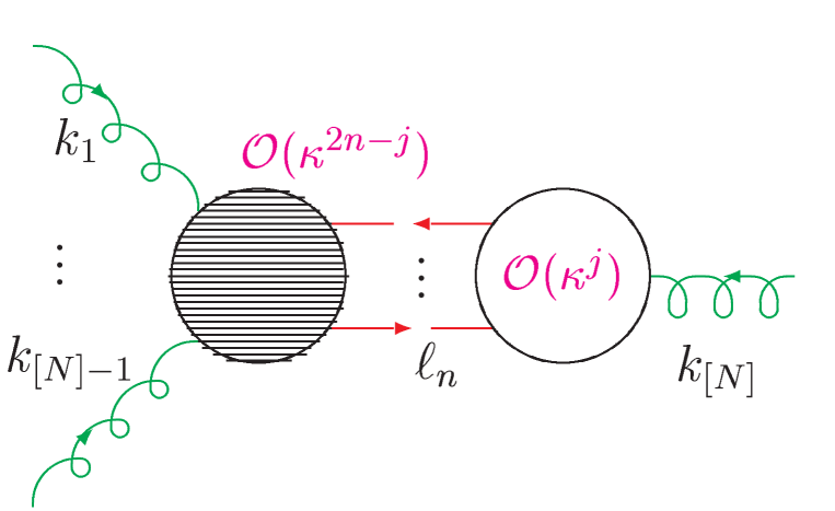
Figure 4: The typical contribution we encounter in $\Gamma_{N}$ at the n-loop level; $\ell_{n}$ is the n-th loop momentum and is precisely the momentum of the indicated resummed improved Born propagator.

We conclude by induction that all $\{\Gamma_{N}\}$ in our theory are finite to all orders in the loop expansion. Of course, the sum of the respective series in $\kappa$ may very well not actually converge but this issue is beyond the scope of our work.

This completes our Appendix.

References

- [1] C. Misner, K.S. Thorne and J.A. Wheeler, Gravitation,( Freeman, San Francisco, 1973 ).
- [2] S. Weinberg, Gravitation and Cosmology: Principles and Applications of the General Theory of Relativity,( John Wiley, New York, 1972).
- [3] S.L. Glashow, Nucl. Phys. 22 (1961) 579; S. Weinberg, Phys. Rev. Lett. 19 (1967) 1264; A. Salam, in Elementary Particle Theory, ed. N. Svartholm (Almqvist and Wiksells, Stockholm, 1968), p. 367.
- [4] G. ’t Hooft and M. Veltman, Nucl. Phys. B44,189 (1972) and B50, 318 (1972); G. ’t Hooft, ibid. B35, 167 (1971); M. Veltman, ibid. B7, 637 (1968).
- [5] D. J. Gross and F. Wilczek, Phys. Rev. Lett. 30 (1973) 1343; H. David Politzer, ibid.30 (1973) 1346; see also , for example, F. Wilczek, in Proc. 16th International Symposium on Lepton and Photon Interactions, Ithaca, 1993, eds. P. Drell and D.L. Rubin (AIP, NY, 1994) p. 593, and references therein.
- [6] C.N. Yang and R.L. Mills, Phys. Rev.96 (1954) 191.
- [7] D. Abbaneo et al., hep-ex/0212036; see also, M. Gruenewald, hep-ex/0210003, in Proc. ICHEP02,eds. S. Bentvelsen et al., (North-Holland,Amsterdam, 2003), Nucl. Phys. B Proc. Suppl. 117(2003) 280; Royal Swedish Academy, ”Press Release: The 1999 Nobel Prize in Physics”, October 12, 1999.
- [8] See, for example, M. Green, J. Schwarz and E. Witten, Superstring Theory, v. 1 and v.2, ( Cambridge Univ. Press, Cambridge, 1987 ) and references therein.
- [9] See, for example, J. Polchinski, String Theory, v. 1 and v. 2, (Cambridge Univ. Press, Cambridge, 1998), and references therein.
- [10] See for example V.N. Melnikov, Gravit. Cosmol. 9, 118 (2003); L. Smolin, hep-th/0303185; A. Ashtekar and J. Lewandowski, Class. Quantum Grav.21 (2004) R53, and references therein.
- [11] R. P. Feynman, Acta Phys. Pol. 24 (1963) 697.
- [12] R. P. Feynman, Feynman Lectures on Gravitation, eds. F.B. Moringo and W.G. Wagner (Caltech, Pasadena, 1971).
- [13] D.J. Gross, hep-th/9704139, in Proc. Conceptual Foundations of Quantum Field Theory, ed. T.Y. Cao (Cambridge Univ. Pr., Cambridge, 1999) p. 56, an references therein.
- [14] J. A. Wheeler, in Relativity, Groups and Topology, eds. B.S. DeWitt and C.M. DeWitt,(Gordon and Breach, New York, 1963) p. 315.
- [15] G. Sterman,Nucl. Phys.B 281, 310 (1987); S. Catani and L. Trentadue, Nucl. Phys.B 327, 323 (1989); ibid. 353, 183 (1991).
- [16] J.C. Collins, D.E. Soper and G. Sterman, Nucl. Phys. B250 (1985) 199.
- [17] J.D. Jackson and D.L. Scharre, Nucl. Instrum. Meth.128(1975) 13; J.D. Jackson, in J.D. Bjorken et al., SLAC-PUB-1515, 1974; Y.-S. Tsai, in ibid., 1974.
- [18] D. R. Yennie, S. C. Frautschi, and H. Suura, Ann. Phys. 13 (1961) 379; see also K. T. Mahanthappa, Phys. Rev. 126 (1962) 329, for a related analysis.
- [19] S. Jadach and B.F.L. Ward, Phys. Rev D38 (1988) 2897; ibid. D39 (1989) 1471; ibid. D40 (1989) 3582; Comput. Phys. Commun.56(1990) 351; Phys.Lett.B274 (1992) 470; S. Jadach et al., Comput. Phys. Commun. 102 (1997) 229; S. Jadach, W. Placzek and B.F.L Ward, Phys.Lett. B390 (1997) 298; S. Jadach, M. Skrzypek and B.F.L. Ward,Phys.Rev. D55 (1997) 1206; S. Jadach, W. Placzek and B.F.L. Ward, Phys. Rev. D56 (1997) 6939; S. Jadach, B.F.L. Ward and Z. Was,Phys. Rev. D63 (2001) 113009; Comp. Phys. Commun. 130 (2000) 260; S. Jadach et al., ibid.140 (2001) 432, 475; S. Jadach, M. Skrzypek and B.F.L. Ward, Phys. Rev. D47 (1993) 3733; Phys. Lett. B257 (1991) 173; in ” Physics”, Proc. XXVth Rencontre de Moriond, Les Arcs, France, 1990, ed. J. Tran Thanh Van (Editions Frontieres, Gif-Sur-Yvette, 1990); S. Jadach et al., Phys. Rev. D44 (1991) 2669; S. Jadach and B.F.L. Ward, preprint TPJU 19/89; in Proc. Brighton Workshop, eds. N. Dombey and F. Boudjema (Plenum, London, 1990), p. 325.
- [20] B.F.L. Ward and S. Jadach, Acta Phys.Polon. B33 (2002) 1543; in Proc. ICHEP2002, ed. S. Bentvelsen et al.,( North Holland, Amsterdam, 2003 ) p. 275; B.F.L. Ward and S. Jadach, Mod. Phys. Lett.A14 (1999) 491; ; D. DeLaney et al., Mod. Phys. Lett. A12 (1997) 2425; D. DeLaney et al.,Phys. Rev. D52 (1995) 108; Phys. Lett. B342 (1995) 239; Phys. Rev. D66 (2002) 019903(E), and references therein.
- [21] C. Glosser et al.,Mod. Phys. Lett. A 19 (2004) 2119; B.F.L. Ward et al., Int. J. Mod. Phys.A20(2005) 3735; in Proc. Beijing 2004, ICHEP 2004, vol. 1, eds. H. Chen et al.,(World Sci. Publ., Singapore, 2005) pp. 588-591; B.F.L. Ward and S. Yost, preprint BU-HEPP-05-05, and references therein.
- [22] S. Weinberg, inGeneral Relativity, eds. S.W. Hawking and W. Israel,( Cambridge Univ. Press, Cambridge, 1979) p.790.
- [23] D.Z. Freedman, P. van Nieuwenhuizen, and S. Ferraro, Phys. Rev. D13 (1976) 3214.
- [24] O. Lauscher and M. Reuter, hep-th/0205062, and references therein.
- [25] A. Bonnanno and M. Reuter, Phys. Rev. D62 (2000) 043008.
- [26] D. Litim, Phys. Rev. Lett.92(2004) 201301; Phys. Rev. D64 (2001) 105007, and references therein.
- [27] R. Percacci and D. Perini, Phys. Rev. D68 (2003) 044018.
- [28] See for example J. Donoghue, Phys. Rev. Lett. 72 (1994) 2996; Phys. Rev. D50 (1994) 3874; preprint gr-qc/9512024; J. Donoghue et al., Phys. Lett. B529 (2002) 132, and references therein.
- [29] See also M. Cavaglia and A. Fabbri, Phys. Rev. D65, 044012 (2002); M. Cavaglia and C. Ungarelli,ibid.61, 064019 (2000), and references therein.
- [30] I. Shapiro and J. Sola, Phys. Lett. B475 (2000) 236; J. High Energy Phys. 0202 (2002) 006; C. Espana-Bonet et al., J. Cos. Astropart. Phys. 0402 (2004) 006; I. Shapiro et al., Phys. Lett. B574 (2003) 149; I. Shapiro, J. Sola and H. Stefancic, ibid. 0501 (2005) 012, and references therein.
- [31] S. Hawking, Nature ( London ) 248 (1974) 30; Commun. Math. Phys. 43 ( 1975 ) 199.
- [32] B.F.L. Ward, Mod. Phys. Lett. A17 (2002) 2371.
- [33] B.F.L. Ward, Mod. Phys. Lett. A19 (2004) 143.
- [34] B.F.L. Ward, J. Cos. Astropart. Phys.0402 (2004) 011.
- [35] B.F.L. Ward, hep-ph/0605054, hep-ph/0503189,0502104, hep-ph/0411050, 0411049, 0410273 and references therein.
- [36] D. Bardin and G. Passarino,The Standard Model in the Making : Precision Study of the Electroweak Interactions , ( Oxford Univ. Press, London, 1999 ).
- [37] F. Gianotti, in Proc. LP2005, eds. R. Brenner et al.,(World Sci. Publ. Co., Singapore, 2006) p. 54; J. Engelen, in Proc. 7th DESY Workshop on Elementary Particle Theory: Loops and Legs in Quantum Field Theory, Nucl. Phys. B Proc. Suppl. 135 (2004) p.3, and refrerences therein.
- [38] B.F.L. Ward, to appear.
- [39] S. Perlmutter et al., Astrophys. J. 517 (1999) 565; and, references therein.
- [40] M. Novello and R. P. Neves, Class. Quant. Grav. 20 (2003) L67; 19 (2002) 5335; J.P. Gazeau and M. Novello, gr-qc/0610054; M. Novello, astro-ph/0504505, and references therein.
- [41] L. D. Faddeev and V.N. Popov, ITF-67-036, NAL-THY-57 (translated from Russian by D. Gordon and B.W. Lee); Phys. Lett. B25 (1967) 29.
- [42] See for example Y. Dokshitzer et al., Rev. Mod. Phys. 60 (1988) 373, and references therein.
- [43] G. ’t Hooft and M. Veltman, Ann. Inst. Henri Poincare XX, 69 (1974).
- [44] See for example D. Wark, in Proc. ICHEP02, in press; and, M. C. Gonzalez-Garcia, hep-ph/0211054, in Proc. ICHEP02, in press, and references therein.
- [45] K. Hagiwara et al., Phys. Rev. D66 (2002) 010001; see also H. Leutwyler and J. Gasser, Phys. Rept. 87 (1982) 77, and references therein.
- [46] S. Eidelman et al., Phys. Lett.B592 (2004) 1.
- [47] See for example M. Yu. Kalmykov and D.I. Kazakov, Phys. Lett.B404(1997) 253; I.L. Buchbinder, S.D. Odintsov and I.L. Shapiro,Effective Action in Quantum Gravity, (IOP Publ.Co.,Bristol and Philadelphia, 1992); and references therein.
- [48] M. Bojowald et al., gr-qc/0503041, and references therein.
- [49] S. Falkenberg and S.D. Odintsov, Int. J. Mod. Phys. A13, 607 (1998).
- [50] T. G. Rizzo, hep-ph/0510420; Class. and Quant. Gravity 23(2006) 4263; J. High Energy Phys. 0609 (2006) 021, also finds that certain higher dimensional TeV-scale gravity theories lead to Planck-scale remnants via the Hawking process.
- [51] J. Linsley, Phys. Rev. Lett. 10(1963) 146; World Data Center for Highest Energy Cosmic Rays, No. 2, Institute of Physical and Chemical Research, Itabashi, Japan; N.N. Efimov et al., Astrophysical Aspects of the Most Energetic Cosmic Rays, eds. M. Nagano and F. Takahara, (World Scientific Publ. Co., Singapore, 1991) p. 20; D. Bird et al., Phys. Rev. Lett. 71(1993) 3401; Astrophys. Journal 424 (1994) 491; M. Takeda et al., Phys. Rev. Lett. 81(1998) 1163, and astro-ph/9902239.
- [52] For a review of the current UHECR data, see S. Westerhoff, in Proc. LP2005, 2005, in press, and references therein.
- [53] S.W. Hawking, in Proc. GR17, 2004, in press.
- [54] D. Z. Freedman and P. van Nieuwenhuizen, Phys. Rev.D14(1976) 912; P. van Nieuwenhuizen, Phys. Repts.68 (1981) 189; and, references therein.
- [55] G. Altarelli, R. Kleiss, and C. Verzegnassi, Z Physics at LEP1, v.1-3, CERN-89-08,(CERN, Geneva, 1989), and references therein.
- [56] H.L. Royden, Real Analysis, (MacMillan Co., New York, 1968).
- [57] S. Weinberg, Phys. Rev. 118 (1960) 838; K. Hepp, Commun. Math. Phys. 2 (1966) 301.