Semi-Inclusive Deep Inelastic Scattering processes from small to large $\mbox{\boldmath$P$}_{T}$

Abstract

We consider the azimuthal and $P_{T}$ dependence of hadrons produced in unpolarized Semi-Inclusive Deep Inelastic Scattering (SIDIS) processes, within the factorized QCD parton model. It is shown that at small $P_{T}$ values, $P_{T}\mathrel{\hbox to0.0pt{\lower 4.0pt\hbox{\hskip 1.0pt$\sim$}\hss}\raise 1.0pt\hbox{$<$}}1$ GeV/$c$, lowest order contributions, coupled to unintegrated (Transverse Momentum Dependent) quark distribution and fragmentation functions, describe all data. At larger $P_{T}$ values, $P_{T}\mathrel{\hbox to0.0pt{\lower 4.0pt\hbox{\hskip 1.0pt$\sim$}\hss}\raise 1.0pt\hbox{$>$}}1$ GeV/$c$, the usual pQCD higher order collinear contributions dominate. Having explained the full $P_{T}$ range of available data, we give new detailed predictions concerning the azimuthal and $P_{T}$ dependence of hadrons which could be measured in ongoing or planned experiments by HERMES, COMPASS and JLab collaborations.

I Introduction

In Ref. sidis1 a comprehensive analysis of Semi-Inclusive Deep Inelastic Scattering (SIDIS) processes within a factorized QCD parton model at $\mathcal{O}(\alpha_{s}^{0})$ was performed in a kinematical scheme in which the intrinsic tranverse momenta of the quarks inside the initial proton ($\mbox{\boldmath$k$}_{\perp}$) and of the final detected hadron with respect to the fragmenting quark ($\mbox{\boldmath$p$}_{\perp}$) were fully taken into account. The dependence of the unpolarized cross section on the azimuthal angle $\phi_{h}$ between the leptonic and the hadron production plane (Cahn effect cahn ) was compared to the available experimental data, and used to estimate the average values of $\langle k_{\perp}^{2}\rangle$ and $\langle p_{\perp}^{2}\rangle$. These values were adopted in modeling the intrinsic motion dependence of the quark distribution and fragmentation functions. This allowed a consistent description of the azimuthal dependence observed by HERMES and COMPASS collaborations in SIDIS off transversely polarized protons herm ; comp , with the subsequent extraction sidis1 ; sidis2 of the Sivers distribution function siv .

In Ref. sidis1 the main emphasis, following the original idea of Cahn, was on the role of the parton intrinsic motion, with the use of unintegrated quark distribution and fragmentation functions. That applies to large $Q^{2}$ processes, in a kinematical regime in which $P_{T}\simeq\Lambda_{\rm QCD}\simeq k_{\perp}$, where $P_{T}=|\mbox{\boldmath$P$}_{T}|$ is the magnitude of the final hadron transverse momentum. In this region QCD factorization with unintegrated distributions holds ji and lowest order QED elementary processes, $\ell\,q\to\ell\,q$, are dominating: the soft $P_{T}$ of the detected hadron is mainly originating from quark intrinsic motion EMC1 ; EMC2 ; E665 , rather than from higher order pQCD interactions, which, instead, would dominantly produce large $P_{T}$ hadrons gp ; chay ; maniatis ; sassot .

Indeed, a look at the results of Ref. sidis1 (see, in particular, Figs. 5 and 6) immediately shows that, while the inclusion of intrinsic $k_{\perp}$ and $p_{\perp}$ – coupled to lowest order partonic interactions – leads to an excellent agreement with the data for small values of the transverse momentum $P_{T}$ of the final hadron, it badly fails at higher $P_{T}$: the turning point is around $P_{T}\sim 1$ GeV/$c$. A similar conclusion was drawn in Ref. chay . The large $P_{T}$ region has been discussed at length in the literature and is related to contributions from higher order QCD processes, like hard gluonic radiation and elementary scatterings initiated by gluons: these cannot be neglected when $P_{T}\gg\lambda_{\rm QCD}$ gp ; chay ; maniatis ; sassot .

In this paper we start by showing that a complete agreement with data in the full range of $P_{T}$ can be achieved; for $P_{T}\mathrel{\hbox to0.0pt{\lower 4.0pt\hbox{\hskip 1.0pt$\sim$}\hss}\raise 1.0pt\hbox{$<$}}1$ GeV/$c$ we follow the approach of Ref. sidis1 – $P_{T}$ originated by the intrinsic $k_{\perp}$ and $p_{\perp}$ with $\mathcal{O}(\alpha_{s}^{0})$ partonic interaction – while in the range of $P_{T}\mathrel{\hbox to0.0pt{\lower 4.0pt\hbox{\hskip 1.0pt$\sim$}\hss}\raise 1.0pt\hbox{$>$}}1$ GeV/$c$ we add the pQCD contributions – collinear partonic configurations with higher order [up to $\mathcal{O}(\alpha_{s}^{2})$] partonic interactions which generate the large $P_{T}$. We shall see that indeed most available data can be explained; the intrinsic $k_{\perp}$ contributions work well at small $P_{T}\mathrel{\hbox to0.0pt{\lower 4.0pt\hbox{\hskip 1.0pt$\sim$}\hss}\raise 1.0pt\hbox{$<$}}1$ GeV/$c$ and fail above that, while the higher order pQCD collinear contributions explain well the large $P_{T}\mathrel{\hbox to0.0pt{\lower 4.0pt\hbox{\hskip 1.0pt$\sim$}\hss}\raise 1.0pt\hbox{$>$}}1$ GeV/$c$ data and fail, or are not even applicable, below that. The two contributions match in the overlapping region, $P_{T}\sim 1$ GeV/$c$, where it might be difficult to disentangle one from the other, as they describe the same physics. Infact parton intrinsic motions originate not only from confinement, but also from soft gluon emission, which, due to QCD helicity conservation, cannot be strictly collinear. Similar studies, concerning single transverse-spin asymmetries in Drell-Yan and SIDIS processes, with separate contributions – TMD quark distributions and higher-twist quark gluon correlations – in separate regions, have recently been published werner1 ; werner2 .

Having achieved such a complete understanding of the $P_{T}$ dependence of the SIDIS cross sections we obtain a full confidence on the regions of applicability of the two approaches. We re-analyse the azimuthal dependence of the unpolarized cross section – the Cahn effect, described in Ref. sidis1 – which depends on quantities integrated over $P_{T}$. The actual data are dominated by the low $P_{T}$ contributions, and the results previously obtained remain valid; we obtain slightly different values of the parameters $\langle k_{\perp}^{2}\rangle$ and $\langle p_{\perp}^{2}\rangle$. We then consider running experiments (HERMES, COMPASS and experiments at JLab) and physical observables which are being or will soon be measured. They are mainly in the small $P_{T}$ regions and we give full sets of predictions for them.

The plan of the paper is the following: in Section II we give a short overview of the kinematics and a collection of the basic formulae needed for the computation of the SIDIS cross sections, both in the low $P_{T}$ approach of Ref. sidis1 and in the pQCD large $P_{T}$ region; in Section III we discuss and compare our results for $d\sigma/dP_{T}$, $d\sigma/d\phi_{h}$ and $\langle\cos\phi_{h}\rangle$ with the existing experimental data, over a very wide range of $P_{T}$ values; in Section IV we give predictions for the forthcoming measurements of $d\sigma/dP_{T}$ and $\langle\cos\phi_{h}\rangle$ at HERMES, Compass and JLab. Some considerations on $\langle\cos 2\phi_{h}\rangle$ are made. Finally, in Section V we draw our conclusions.

II Kinematics and Cross Sections

We consider SIDIS processes $\ell\,p\to\ell\,h\,X$ in the $\gamma^{*}p$ c.m. frame, as shown in Fig. 1. The photon and the proton collide along the $z$ axis with momenta $q$ and $P$ respectively; the leptonic plane coincides with the $x$-$z$ plane. We adopt the usual SIDIS variables (neglecting all masses):

$$s=(P+\ell)^{2}\quad\quad(P+q)^{2}=W^{2}=\frac{1-x_{{}_{\!B\!j}}}{x_{{}_{\!B\!j}}}\,Q^{2}\quad\quad q^{2}=-Q^{2}$$

$$x_{{}_{\!B\!j}}=\frac{Q^{2}}{2P\cdot q}=\frac{Q^{2}}{W^{2}+Q^{2}}\quad\quad y=\frac{P\cdot q}{P\cdot\ell}=\frac{Q^{2}}{x_{{}_{\!B\!j}}s}\quad\quad z_{h}=\frac{P\cdot P_{h}}{P\cdot q}\>\cdot$$ (1)

Figure 1: Three dimensional kinematics of the SIDIS process.

The SIDIS differential cross section can schematically be written in terms of a perturbative expansion in orders of $\alpha_{s}$ as follows

$$d\sigma\;=\;\alpha_{s}^{0}\;d\sigma_{0}+\ \alpha_{s}^{1}\;d\sigma_{1}+\alpha_{s}^{2}\;d\sigma_{2}+...\,,$$ (2)

where $d\sigma$ is a short hand notation to indicate $\displaystyle{\frac{d^{5}\sigma^{\ell p\to\ell hX}}{dx_{{}_{\!B\!j}}\,dy\,dz_{h}\,d^{2}\mbox{\boldmath$P$}_{T}}}=x_{{}_{\!B\!j}}s\,{\frac{d^{5}\sigma^{\ell p\to\ell hX}}{dx_{{}_{\!B\!j}}\,dQ^{2}\,dz_{h}\,d^{2}\mbox{\boldmath$P$}_{T}}}\cdot$

The first term in this expansion is the lowest order one; in the elementary interaction, $\ell\,q\to\ell\,q$, a virtual photon with four-momentum $q$ strikes a quark which carries a transverse momentum $\mbox{\boldmath$k$}_{\perp}=k_{\perp}(\cos\varphi,\sin\varphi,0)$ in addition to a fraction $x$ of the light-cone proton momentum. The final detected hadron $h$ originates from the fragmentation of the outgoing quark: $\mbox{\boldmath$p$}_{\perp}$ is the transverse momentum of $h$ with respect to the direction of the fragmenting quark and $z$ is the fraction of the light-cone quark momentum carried by the resulting hadron. Consequently, the detected hadron can have a transverse momentum $\mbox{\boldmath$P$}_{T}$ with a magnitude $P_{T}\simeq\langle k_{\perp}\rangle\simeq\langle p_{\perp}\rangle$. Indeed, this is the main source of hadrons with a small value of $P_{T}$ chay ; EMC1 ; EMC2 ; E665 .

Such a mechanism translates into a factorized ji expression for the SIDIS cross section, valid at all orders in $(k_{\perp}/Q)$:

$$\frac{d^{5}\sigma^{\ell p\to\ell hX}_{0}}{dx_{{}_{\!B\!j}}\,dQ^{2}\,dz_{h}\,d^{2}\mbox{\boldmath$P$}_{T}} =\sum_{q}\int{d^{2}\mbox{\boldmath$k$}_{\perp}}\;f_{q}(x,\mbox{\boldmath$k$}_{\perp})\;\frac{d\hat{\sigma}^{\ell q\to\ell q}}{dQ^{2}}\;J\;\frac{z}{z_{h}}\;D_{q}^{h}(z,\mbox{\boldmath$p$}_{\perp})$$ (3)

$$=\sum_{q}e_{q}^{2}\int\!d^{2}\mbox{\boldmath$k$}_{\perp}\;f_{q}(x,\mbox{\boldmath$k$}_{\perp})\;\frac{2\pi\alpha^{2}}{x_{{}_{\!B\!j}}^{2}s^{2}}\,\frac{\hat{s}^{2}+\hat{u}^{2}}{Q^{4}}\;D_{q}^{h}(z,\mbox{\boldmath$p$}_{\perp})\;\frac{z}{z_{h}}\,\frac{x_{{}_{\!B\!j}}}{x}\left(1+\frac{x_{{}_{\!B\!j}}}{x}\frac{k_{\perp}^{2}}{Q^{2}}\right)^{\!\!-1}\>,$$

as explained in Ref. sidis1 , where the exact relationships between $x,z,\mbox{\boldmath$p$}_{\perp}$ and the observables $x_{{}_{\!B\!j}},z_{h},\mbox{\boldmath$P$}_{T}$ are given. Notice that at $\mathcal{O}(k_{\perp}/Q)$ one has $x_{{}_{\!B\!j}}=x$, $z_{h}=z$ and $\mbox{\boldmath$P$}_{T}=z\mbox{\boldmath$k$}_{\perp}+\mbox{\boldmath$p$}_{\perp}$. $f_{q}(x,\mbox{\boldmath$k$}_{\perp})$ and $D_{q}^{h}(z,\mbox{\boldmath$p$}_{\perp})$ are the parton density and the fragmentation function respectively, for which we assume the usual $x,k_{\perp}$ or $z,p_{\perp}$ factorization, with a gaussian $k_{\perp}$ and $p_{\perp}$ dependence:

$$f_{q}(x,\mbox{\boldmath$k$}_{\perp})=f_{q}(x)\,\frac{1}{\pi\langle k_{\perp}^{2}\rangle}\,e^{-{k_{\perp}^{2}}/{\langle k_{\perp}^{2}\rangle}}\quad\quad D_{q}^{h}(z,\mbox{\boldmath$p$}_{\perp})=D_{q}^{h}(z)\,\frac{1}{\pi\langle p_{\perp}^{2}\rangle}\,e^{-{p_{\perp}^{2}}/\langle p_{\perp}^{2}\rangle}\,,$$ (4)

so that

$$\int d^{2}\mbox{\boldmath$k$}_{\perp}\>f_{q}(x,\mbox{\boldmath$k$}_{\perp})=f_{q}(x)\quad\quad\int d^{2}\mbox{\boldmath$p$}_{\perp}\>D_{q}^{h}(z,\mbox{\boldmath$p$}_{\perp})=D_{q}^{h}(z)\>.$$ (5)

The integration over $d^{2}\mbox{\boldmath$k$}_{\perp}$ in Eq. (3) induces a dependence on $\cos\phi_{h}$ [at $\mathcal{O}(P_{T}/Q)$] and on $\cos 2\phi_{h}$ [at $\mathcal{O}(P_{T}/Q)^{2}$], where $\phi_{h}$ is the azimuthal angle of $\mbox{\boldmath$P$}_{T}$. The explicit expression, at $\mathcal{O}(P_{T}/Q)$, is given by:

$$\frac{d^{5}\sigma^{\ell p\to\ell hX}}{dx_{{}_{\!B\!j}}\,dQ^{2}\,dz_{h}\,d^{2}\mbox{\boldmath$P$}_{T}}\simeq\sum_{q}\frac{2\pi\alpha^{2}e_{q}^{2}}{Q^{4}}\>f_{q}(x_{{}_{\!B\!j}})\>D_{q}^{h}(z_{h})\,\biggl{[}1+(1-y)^{2}$$

$$\hskip 36.0pt-4\>\frac{(2-y)\sqrt{1-y}\>\langle k_{\perp}^{2}\rangle\,z_{h}\,P_{T}}{\langle P_{T}^{2}\rangle\,Q}\>\cos\phi_{h}\biggr{]}\frac{1}{\pi\langle P_{T}^{2}\rangle}\,e^{-P_{T}^{2}/\langle P_{T}^{2}\rangle}\,.$$ (6)

where, $\langle P_{T}^{2}\rangle=\langle p_{\perp}^{2}\rangle+z^{2}\langle k_{\perp}^{2}\rangle$.

Let us now consider the contributions of order $\alpha_{s}$, $d\sigma_{1}$ in Eq. (2). We follow the approach of Ref. chay . The relevant partonic processes, shown in Fig. 2, are those in which the quark emits a hard gluon or those initiated by gluons:

$$\gamma^{*}\,+\,q\to q\,+\,g\quad\quad\gamma^{*}\,+\,q\to g\,+\,q\quad\quad\gamma^{*}\,+\,g\to q\,+\,\bar{q}\,.$$ (7)

It is clear that now, contrary to the lowest order QED process, $\gamma^{*}\,+\,q\to q$, the final parton can have a large transverse momentum, even starting from a collinear configuration. Such a contribution certainly dominates the production of hadrons with large $P_{T}$ values.

One introduces the parton variables $x^{\prime}$ and $z^{\prime}$, defined similarly to the hadronic variables $x_{{}_{\!B\!j}}$ and $z_{h}$,

$$x^{\prime}=\frac{Q^{2}}{2k\cdot q}=\frac{x_{{}_{\!B\!j}}}{\xi}\quad\quad z^{\prime}=\frac{k\cdot k^{\prime}}{k\cdot q}=\frac{z_{h}}{\zeta}\,,$$ (8)

where $k$ and $k^{\prime}$ are the four-momenta of the incident and fragmenting partons respectively. $\xi$ and $\zeta$ are the usual light-cone momentum fractions, which, in the collinear configuration with massless partons are given by $k=\xi P$ and $P_{h}=\zeta k^{\prime}$. We denote by $\mbox{\boldmath$p$}_{T}$ (not to be confused with $\mbox{\boldmath$p$}_{\perp}$) the transverse momentum, with respect to the $\gamma^{*}$ direction, of the final fragmenting parton, $\mbox{\boldmath$P$}_{T}=\zeta\mbox{\boldmath$p$}_{T}$.

The semi-inclusive DIS cross section, in the QCD parton model with collinear configuration, can be written, in general, as:

$$\frac{d^{5}\sigma^{lp\rightarrow lhX}}{dx_{{}_{\!B\!j}}dy\,dz_{h}\,d^{2}\mbox{\boldmath$P$}_{T}} = \sum_{i,j}\int dx^{\prime}\,dz^{\prime}\,d^{2}\mbox{\boldmath$p$}_{T}\,d\xi\,d\zeta\delta\left(x_{{}_{\!B\!j}}-\xi x^{\prime}\right)\delta\left(z_{h}-\zeta z^{\prime}\right)\delta^{2}\left(\mathbf{P}_{T}-\zeta\mbox{\boldmath$p$}_{T}\right)$$ (9)

$$\times f_{i}\left(\xi,Q^{2}\right)\frac{d\hat{\sigma}_{ij}}{dx^{\prime}\,dy\,dz^{\prime}\,d^{2}\mbox{\boldmath$p$}_{T}}D_{j}^{h}\left(\zeta,Q^{2}\right)\,.$$

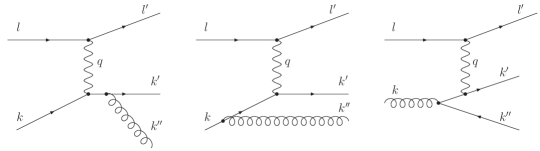
Figure 2:

Feynman diagrams corresponding to $\ell q$ and $\ell g$ elementary scattering at first order in $\alpha_{s}$.

To first order in $\alpha_{s}$ the partonic cross section is given by mendez-kroll ; chay

$$\frac{d\hat{\sigma}_{ij}}{dx^{\prime}\,dy\,dz^{\prime}\,d^{2}\mbox{\boldmath$p$}_{T}}=\frac{\alpha^{2}e_{q}^{2}}{16\pi^{2}Q^{4}}\,y\,L_{\mu\nu}M_{ij}^{\mu\nu}\delta\left(p^{2}_{T}-\frac{z^{\prime}}{x^{\prime}}(1-x^{\prime})(1-z^{\prime})Q^{2}\right),$$ (10)

where $ij$ denote the initial and fragmenting partons, $ij=qq,qg,gq$. Inserting the above expression into Eq. (9) yields, for the $\mathcal{O}(\alpha_{s})$ cross section:

$$\frac{d^{5}\sigma^{lp\rightarrow lhX}_{1}}{dx_{{}_{\!B\!j}}dy\,dz_{h}\,d^{2}\mbox{\boldmath$P$}_{T}}=\frac{\alpha^{2}\,e_{q}^{2}}{16\pi^{2}}\,\frac{y}{Q^{4}}\int_{x_{{}_{\!B\!j}}}^{1}\frac{dx^{\prime}}{x^{\prime}P_{T}^{2}+z_{h}^{2}(1-x^{\prime})Q^{2}}\sum_{i,j}f_{i}\left(\frac{x_{{}_{\!B\!j}}}{x^{\prime}},Q^{2}\right)\,L_{\mu\nu}\,M_{ij}^{\mu\nu}\,D_{j}^{h}\left(z_{h}+\frac{x^{\prime}P_{T}^{2}}{z_{h}(1-x^{\prime})Q^{2}},Q^{2}\right)\,$$ (11)

with chay

$$L_{\mu\nu}M_{qq}^{\mu\nu} = \frac{64\pi}{3}Q^{2}\frac{(l\cdot k)^{2}+(l^{\prime}\cdot k^{\prime})^{2}+(l^{\prime}\cdot k)^{2}+(l\cdot k^{\prime})^{2}}{(k\cdot k^{\prime\prime})(k^{\prime}\cdot k^{\prime\prime})}$$ (12)

$$= \frac{64\pi}{3}\,\frac{Q^{2}}{y^{2}}\,\left\{[1+(1-y)^{2}]\;\left[(1-x^{\prime})(1-z^{\prime})+\frac{1+(x^{\prime}z^{\prime})^{2}}{(1-x^{\prime})(1-z^{\prime})}\right]\,+\,8\,x^{\prime}z^{\prime}\;(1-y)\right.$$

$$\left.-\;4\,\sqrt{\frac{x^{\prime}z^{\prime}\;(1-y)}{(1-x^{\prime})(1-z^{\prime})}}\;(2-y)\;[x^{\prime}z^{\prime}+(1-x^{\prime})(1-z^{\prime})]\cos\phi_{h}\right.$$

$$\left.+\;4\,x^{\prime}z^{\prime}\,(1-y)\,\cos 2\phi_{h}\frac{}{}\right\}\;,$$

$$L_{\mu\nu}M_{qg}^{\mu\nu} = \frac{64\pi}{3}Q^{2}\frac{(l\cdot k)^{2}+(l^{\prime}\cdot k^{\prime\prime})^{2}+(l^{\prime}\cdot k)^{2}+(l\cdot k^{\prime\prime})^{2}}{(k\cdot k^{\prime})(k^{\prime}k^{\prime\prime})}$$ (13)

$$= \frac{64\pi}{3}\,\frac{Q^{2}}{y^{2}}\,\left\{[1+(1-y)^{2}]\;\left[(1-x^{\prime})z^{\prime}+\frac{1+{x^{\prime}}^{2}(1-z^{\prime})^{2}}{(1-x^{\prime})z^{\prime}}\right]\,+\,8\,x^{\prime}(1-y)(1-z^{\prime})\right.$$

$$\left.+\;4\,\sqrt{\frac{x^{\prime}(1-y)(1-z^{\prime})}{(1-x^{\prime})z^{\prime}}}\;(2-y)\;[x^{\prime}(1-z^{\prime})+(1-x^{\prime})z^{\prime}]\cos\phi_{h}\right.$$

$$\left.+\;4\,x^{\prime}(1-y)(1-z^{\prime})\,\cos 2\phi_{h}\frac{}{}\right\}\;,$$

$$L_{\mu\nu}M_{gq}^{\mu\nu} = \frac{64\pi}{3}Q^{2}\frac{(l\cdot k^{\prime\prime})^{2}+(l^{\prime}\cdot k^{\prime})^{2}+(l^{\prime}\cdot k^{\prime\prime})^{2}+(l\cdot k^{\prime})^{2}}{(k\cdot k^{\prime})(k\cdot k^{\prime\prime})}$$ (14)

$$= 8\pi\alpha_{s}\;\frac{Q^{2}}{y^{2}}\left\{[1+(1-y)^{2}]\;[{x^{\prime}}^{2}+(1-x^{\prime})^{2}]\;\frac{{z^{\prime}}^{2}+(1-z^{\prime})^{2}}{z^{\prime}(1-z^{\prime})}\,+\,16\,x^{\prime}(1-x^{\prime})(1-y)\right.$$

$$\left.-\;4\,\sqrt{\frac{x^{\prime}(1-x^{\prime})(1-y)}{z^{\prime}(1-z^{\prime})}}\;(2-y)\;(1-2x^{\prime})(1-2z^{\prime})\,\cos\phi_{h}\right.$$

$$\left.+\;8\,x^{\prime}(1-x^{\prime})(1-y)\,\cos 2\phi_{h}\frac{}{}\right\}\;,$$

where we have explicitely written the scalar products in terms of $x^{\prime}$, $y$, $z^{\prime}$ and $\cos\phi_{h}$. Notice the appearance of the $\cos\phi_{h}$ and $\cos 2\phi_{h}$ terms: $\phi_{h}$ is the azimuthal angle of the fragmenting partons, which, in a collinear configuration, concides with the azimuthal angle of the detected final hadron. The above expressions agree with results previously obtained in the literature mendez-kroll .

Large values of $P_{T}$ cannot be generated by the modest amount of intrinsic motion sidis1 ; we expect that Eq.(11) will dominantly describe the cross sections for the lepto-production of hadrons with $P_{T}$ values above $1$ (GeV/c).

Let us finally briefly consider the contributions of order $\alpha_{s}^{2}$ (NLO), $d\sigma_{2}$ in Eq. (2). These, for the production of large $P_{T}$ hadrons, have been recently computed maniatis ; sassot , resulting in large corrections to the $\mathcal{O}(\alpha_{s})$ (LO) results, and leading to a good agreement with experimental data. It would be unnecessarily complicated, for our purposes, to take exactly into account these contributions, as we have done for the LO ones, via Eqs. (11)–(14). The most simple way of inserting the NLO results in our study is via the $K$ factor, defined as the NLO to LO ratio of the SIDIS cross sections. A close examination of the $K$ factor shows a clear dependence on $P_{T}$ and the other kinematical variables: for example, it may be larger than $10$ at low $P_{T}$ and $Q^{2}$, while approaching unity at larger values (see, for example, Fig. 3 of Ref. maniatis ). However, we shall need to use the $K$ factor only in limited ranges of $P_{T}$ (up to 3 GeV/$c$ at most) and $Q^{2}$, depending on the sets of experimental data we consider: in these limited kinematical regions we find that a satisfactory description of the SIDIS experimental data can be achieved by using constant values of $K$, which will be indicated in each case.

Therefore, we will effectively include $\mathcal{O}(\alpha_{s}^{2})$ contributions in our computations by writing Eq. (2) as

$$d\sigma=\alpha_{s}^{0}d\sigma_{0}+\ \alpha_{s}^{1}\,K\,d\sigma_{1}+...\,,$$ (15)

where $d\sigma_{0}$ and $d\sigma_{1}$ are calculated according to Eqs. (3) and (11) respectively. The first term dominates at $P_{T}\mathrel{\hbox to0.0pt{\lower 4.0pt\hbox{\hskip 1.0pt$\sim$}\hss}\raise 1.0pt\hbox{$<$}}1$ GeV/$c$, and the second one at $P_{T}\mathrel{\hbox to0.0pt{\lower 4.0pt\hbox{\hskip 1.0pt$\sim$}\hss}\raise 1.0pt\hbox{$>$}}1$ GeV/$c$.

III Numerical Results

In Ref. sidis1 several sets of experimental data, showing the explicit dependence of the SIDIS unpolarized cross sections on the azimuthal angle $\phi_{h}$ and on $P_{T}$, were considered. A comprehensive fit, based on Eq. (3) – or its simplified version valid up to $\mathcal{O}(k_{\perp}/Q)$, Eq. (6) – was performed, in order to determine the values of $\langle k_{\perp}^{2}\rangle$ and $\langle p_{\perp}^{2}\rangle$, obtaining

$$\langle k_{\perp}^{2}\rangle=0.25\;({\rm GeV})^{2}\quad\quad\langle p_{\perp}^{2}\rangle=0.20\;({\rm GeV})^{2}\>.$$

These values were assumed to be constant and flavour independent.

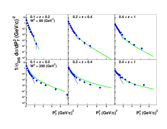
Figure 3: The normalized cross section $d\sigma/dP_{T}^{2}$: the dashed line reproduces the $\mathcal{O}(\alpha_{s}^{0})$ contributions, computed by taking into account the partonic transverse intrinsic motion at all orders in $(k_{\perp}/Q)$, Eq. (3). The solid line corresponds to collinear and pQCD contributions, computed at LO, with a $K$ factor ($K=6$) to account for NLO effects, Eqs. (11)-(15). The data are from EMC collaboration measurements EMCpt . $\langle k_{\perp}\rangle$ and $\langle p_{\perp}\rangle$ are fixed as in Eq. (III).

The study of Ref. sidis1 also showed clearly that Eq. (3) – zeroth order pQCD with TMD distribution and fragmentation function – works very well in the $P_{T}\simeq\Lambda_{\rm QCD}\simeq k_{\perp}$ region, but fails at larger $P_{T}$ values, where higher order pQCD contributions, with collinear partonic configurations, are expected to take over and explain the data. The transition point is around $P_{T}\simeq 1$ GeV/$c$.

We have redone the analysis of Ref. sidis1 taking into account, in the appropriate kinematical regions, also the pQCD contributions. It turns out that, while a complete description of the data in the full $P_{T}$ range is possible, a little variation is required to the values given in Eq. (III). Actually, the resulting change is included within a 20% variation of the parameters, already considered in Ref. sidis1 .

Figs. 3-7 show our results obtained by adding, according to Eq. (15), the contributions of Eq. (3) to the contributions (computed above $P_{T}=1$ GeV/$c$) of Eq. (11). We have used

$$\langle k_{\perp}^{2}\rangle=0.28\;({\rm GeV})^{2}\quad\quad\langle p_{\perp}^{2}\rangle=0.25\;({\rm GeV})^{2}\>,$$

again constant and flavour independent. The $K$ factor was fixed to be a constant, with different values according to the different $P_{T}$ and $Q^{2}$ ranges involved. Here and throughout the paper we have adopted the MRST01 NLO MRST01 set of distribution functions and the fragmentation functions by Kretzer Kretzer at NLO.

Let us comment in greater detail on each single plot. In Fig. 3 we compare our results to the EMC measurements of the SIDIS $P_{T}^{2}$ distributions (normalized to the integrated DIS cross section) EMCpt , defined as

$$\frac{1}{\sigma_{{}_{\rm DIS}}}\frac{d\sigma}{dP_{T}^{2}}=\frac{1}{2\sigma_{{}_{\rm DIS}}}\,\int\!d\phi_{h}\,dx_{{}_{\!B\!j}}\,dy\,dz_{h}\frac{d^{5}\sigma^{\ell p\to\ell hX}}{dx_{{}_{\!B\!j}}\,dy\,dz_{h}\,d^{2}\mbox{\boldmath$P$}_{T}},$$ (16)

where the integration covers the $x_{{}_{\!B\!j}}$, $y$, $z_{h}$ and $P_{T}$ regions consistent with the experimental cuts:

$$Q^{2}>5\;({\rm GeV}/c)^{2}\quad\quad E_{h}>5\;({\rm GeV})\quad\quad 0.1<z_{h}<1\quad\quad 0.2<y<0.8\,.$$

The dashed lines reproduce the $\mathcal{O}(\alpha_{s}^{0})$ contribution, computed by taking into account the partonic transverse intrinsic motion at all orders in $(k_{\perp}/Q)$, whereas the solid lines correspond to the SIDIS cross section as obtained by including LO corrections and the $K$ factor ($K=6$) to account for NLO effects. The two contributions together give a very good complementary description of the data over the full $P_{T}$ domain. Unavoidably, there is a slight mismatch at the transition point, $P_{T}=1$ GeV/$c$, where both contributions somewhat describe the same physics, and some kind of average should be performed to avoid double counting. The value $K=6$ is the simplest, although rough, approximation, in the kinematical range of the data considered here, to the computed $K$ factor (see, Fig. 3 of Ref. maniatis ). $\sigma_{{}_{\rm DIS}}$ is evaluated starting from Eq. (17) of Ref. sidis1 ; pQCD corrections for this integrated quantity are negligible.

A similar very good agreement, shown in Fig. 4, is obtained when comparing our computations with the experimental measurements of the ZEUS collaboration at DESY Derrick96 . Here the SIDIS differential cross section,

$$\frac{1}{\sigma_{{}_{\rm DIS}}}\frac{d\sigma}{dP_{T}}=\frac{1}{\sigma_{{}_{\rm DIS}}}\,\int\!d\phi_{h}\;dx_{{}_{\!B\!j}}dQ^{2}dz_{h}P_{T}\frac{d^{5}\sigma^{\ell p\to\ell hX}}{dx_{{}_{\!B\!j}}\,dQ^{2}\,dz_{h}\,d^{2}\mbox{\boldmath$P$}_{T}}\>,$$ (17)

is obtained by performing the integrations according to the following experimental conditions

$$10<Q^{2}<160\;({\rm GeV}/c)^{2}\quad\quad 75<W<175\;({\rm GeV})\>,$$ (18)

and the $K$ factor is taken to be 1.5 (as shown in Fig. 8 of Ref. maniatis ).

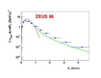
Figure 4: The normalized cross section $d\sigma/dP_{T}$: the dashed line reproduces the $\mathcal{O}(\alpha_{s}^{0})$ contribution, computed by taking into account the partonic transverse intrinsic motion at all orders in the $(k_{\perp}/Q)$ expansion, Eq. (3); the solid line corresponds to the SIDIS cross section as given by LO contributions and a $K$ factor ($K=1.5$) to account for NLO effects, Eqs. (11)–(15). The data are from ZEUS collaboration measurements Derrick96 . $\langle k_{\perp}\rangle$ and $\langle p_{\perp}\rangle$ are fixed as in Eq. (III).

In Fig. 5 we compare our results to the EMC measurements of the (not normalized) $\phi_{h}$ distributions EMC2 , proportional to

$$\frac{d\sigma^{\ell p\to\ell hX}}{d\phi_{h}}=\int\!dx_{{}_{\!B\!j}}\,dy\,dz_{h}\,P_{T}\,dP_{T}\;\frac{d^{5}\sigma^{\ell p\to\ell hX}}{dx_{{}_{\!B\!j}}\,dy\,dz_{h}\,d^{2}\mbox{\boldmath$P$}_{T}}\,.$$ (19)

The integration regions are fixed by the conditions

$$x_{F}>0.1\quad\quad P_{T}>0.2\;({\rm GeV}/c)\quad\quad 0.2<y<0.8\quad\quad Q^{2}>\;4({\rm GeV}/c)^{2}\,,$$

where $x_{F}={2P_{L}}/{W}\,$ and $P_{L}$ is the longitudinal momentum of the produced hadron relative to the virtual photon.

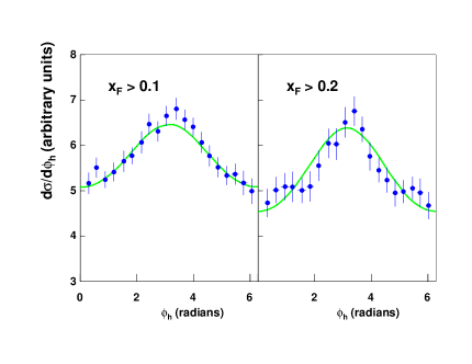
Figure 5: The cross section $d\sigma/d\phi_{h}$: the solid line is obtained by including all orders in $(k_{\perp}/Q)$, the LO corrections and a $K=6$ factor to account for NLO effects. The data are from EMC measurements EMC2 . $\langle k_{\perp}\rangle$ and $\langle p_{\perp}\rangle$ are fixed as in Eq. (III).

This is a quantity integrated over $P_{T}\geq 0.2$ GeV/$c$; we have used only $d\sigma_{0}$ up to $P_{T}=1$ GeV/$c$ and added the $K\,d\sigma_{1}$ contributions (with $K=6$) above that. We notice, however, that the dominant contributions come from very low $P_{T}$’s, while the pQCD contribution is almost negligible.

Figs. 6 and 7 show our predictions for the average value of $\cos\phi_{h}$ compared to the experimental data from the FNAL E665 collaboration E665 ($\mu p$ and $\mu d$ interactions at $490$ GeV) and from the ZEUS collaboration Breitweg (positron-proton collisions at $300$ GeV) respectively. Here $\langle\cos\phi_{h}\rangle$ is defined as

$$\langle\cos\phi_{h}\rangle=\frac{\int dx_{{}_{\!B\!j}}dQ^{2}dz_{h}d^{2}\mbox{\boldmath$P$}_{T}\;\cos\phi_{h}\;d^{5}\sigma}{\int dx_{{}_{\!B\!j}}dQ^{2}dz_{h}d^{2}\mbox{\boldmath$P$}_{T}\;d^{5}\sigma}\,,$$ (20)

where $d^{5}\sigma$ denotes the fully differential cross section

$$d^{5}\sigma\equiv\frac{d^{5}\sigma^{\ell p\to\ell hX}}{dx_{{}_{\!B\!j}}\,dQ^{2}\,dz_{h}\,d^{2}\mbox{\boldmath$P$}_{T}}\,\cdot$$ (21)

For the FNAL E665 data sample the integral over $P_{T}$ runs from $P_{T}^{cut}$ to $P_{T}^{max}\sim 10$ GeV/$c$ and the range of the other variables is fixed by the following experimental cuts:

$$Q^{2}>3\;{\rm(GeV)^{2}}\;,\;\;\;300<W^{2}<900\;{\rm(GeV)^{2}}\;,$$

$$60<\nu<500\;{\rm(GeV)}\;,\;\;\;E_{h}>8\;{\rm(GeV)}\;,\;\;\;0.1<y<0.85\,,$$ (22)

whereas for the ZEUS data sample the integral over $P_{T}$ runs from $P_{T}^{cut}$ to $P_{T}^{max}\sim 10$ GeV/$c$, within the ranges

$$0.01<x_{{}_{\!B\!j}}<0.1\;,\;\;\;0.2<y<0.8\;,$$

$$0.2<z_{h}<1.0\;,\;\;\;180<Q^{2}<7220\;{\rm(GeV)^{2}}\;.$$ (23)

As in the previous case, we have added perturbative corrections only from $P_{T}=1$ (GeV/$c$), leaving $d\sigma_{0}$ to be the only contributing term for values of $P_{T}$ below $1$ (GeV/$c$).

The results we obtain are in good qualitative agreement with the FNAL E665 experimental data. As expected, they show that the pQCD contributions are very small at low $P_{T}^{cut}$ values, but quickly increase as $P_{T}^{cut}$ raises, significantly correcting the fast fall of the $\mathcal{O}(\alpha_{s}^{0})$ term, as shown in Fig. 6.

Instead, our results disagree with the ZEUS data, especially in the lower range of $P_{T}^{\rm cut}$. This is surprising and would deserve further experimental studies. The $\cos\phi_{h}$ modulation, at small $P_{T}$ values, is a kinematical higher-twist effect, and decreases like $P_{T}/Q$ for growing values of $Q$, as shown in Eq. (6). Therefore we expect, and indeed we find, $\langle\cos\phi_{h}\rangle$ to be much smaller for ZEUS data, which correspond to huge values of $Q^{2}$, than for E665 results, which correspond to much lower $Q^{2}$ values.

We have also computed, with the same procedure, $\langle\cos(2\phi_{h})\rangle$. We have seen that such a dependence can arise both, at $\mathcal{O}(P_{T}/Q)^{2}$, from intrinsic motion, and, at $\mathcal{O}(\alpha_{s})$, from pQCD corrections. However, there is another non perturbative, leading-twist, small $P_{T}$ source of the $\cos(2\phi_{h})$ dependence, related to the combined action of the Boer-Mulders bm and Collins col effects; this has been recently studied in Ref bar , where both the $1/Q^{2}$ kinematical contribution and the Boer-Mulders $\otimes$ Collins one were studied and found to be of comparable size. Therefore, our results, which ignore the Boer-Mulders $\otimes$ Collins contribution, can be considered reliable only in the large $P_{T}$ region; indeed, in this region, we find agreement with the ZEUS experimental data of Ref. Breitweg , as shown in Fig. 8.

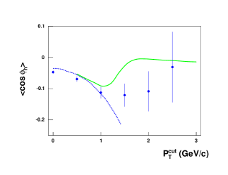
Figure 6: $\langle\cos\phi_{h}\rangle$ as a function of $P_{T}^{cut}$: the dashed line reproduces the $\mathcal{O}(\alpha_{s}^{0})$ contribution, computed by taking into account the partonic transverse intrinsic motion at all orders in $(k_{\perp}/Q)$; the solid line corresponds to the SIDIS cross section as obtained by including LO corrections and a $K=6$ factor to account for NLO effects. The data are from the E665 collaboration E665 .

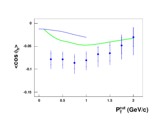
Figure 7: $\langle\cos\phi_{h}\rangle$ as a function of $P_{T}^{cut}$: the dashed line reproduces the $\mathcal{O}(\alpha_{s}^{0})$ contribution, computed by taking into account the partonic transverse intrinsic motion at all orders in $(k_{\perp}/Q)$; the solid line corresponds to the SIDIS cross section as obtained by including LO corrections and a $K=1.5$ factor to account for NLO effects. The data are from the ZEUS collaboration Breitweg .

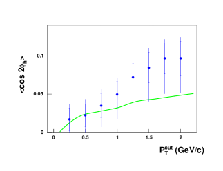
Figure 8: $\langle\cos(2\phi_{h})\rangle$ as a function of $P_{T}^{cut}$ as obtained by including LO corrections and a $K=1.5$ factor to account for NLO effects. The data are from the ZEUS collaboration Breitweg .

IV Predictions for forthcoming measurements

New data are expected from ongoing measurements or data analysis at HERMES, COMPASS and JLab. They concern dominantly the small $P_{T}$ (and, hopefully, large enough $Q^{2}$) region, where we have seen that the simple partonic approach, with unintegrated distribution and fragmentation functions, can give a very satisfactory description of the available data. We can easily give detailed predictions which can soon be tested, allowing a further check on the role of intrinsic motions in affecting physical observables. We consider the SIDIS cross sections and the average value of $\cos\phi_{h}$. Also $\langle\cos 2\phi_{h}\rangle$, keeping in mind the comments at the end of the previous Section, is computed.

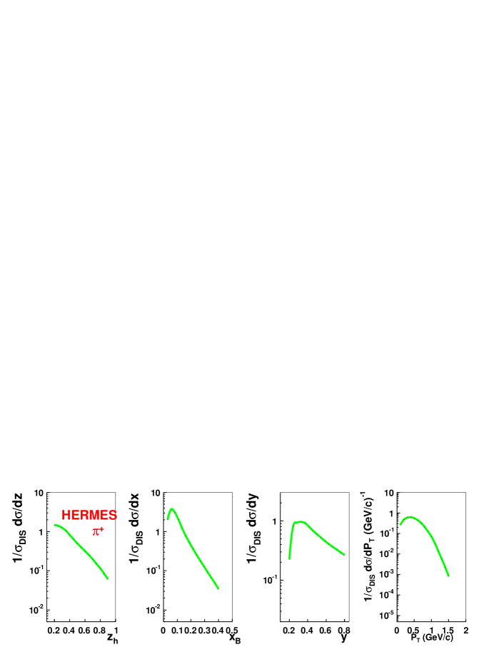
Figure 9: Predictions for the normalized SIDIS cross section corresponding to the production of $\pi^{+}$ as it will be measured by the HERMES collaboration in the forthcoming future. The solid lines correspond to the SIDIS cross section as obtained by including all orders in the $(k_{\perp}/Q)$ expansion. Notice that QCD corrections have no influence in this range of low $P_{T}$’s.

In Fig. 9, we plot the SIDIS cross section, for $\pi^{+}$ production at HERMES, as function of one variable at a time, either $z_{h}$, $x_{{}_{\!B\!j}}$, $y$ or $P_{T}$; the integration over the unobserved variables has been performed consistently with the setup of the HERMES experiment, which studies the scattering of positrons at $p_{lab}=27.57$ GeV/$c$ against a fixed hydrogen gas target:

$$Q^{2}>1\;({\rm GeV}/c)^{2}\quad\quad W^{2}>10\;{\rm GeV}^{2}\quad\quad P_{T}>0.05\;{\rm GeV}/c$$

$$0.023<x_{{}_{\!B\!j}}<0.4\quad\quad 0.2<z_{h}<0.7\quad\quad 0.1<y<0.85\quad\quad 2<E_{h}<15\>{\rm GeV}\>.$$ (24)

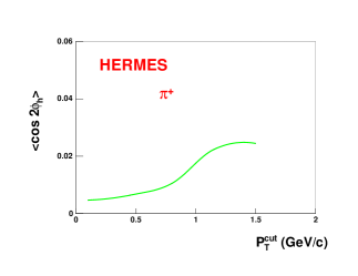
Figure 11: Predictions for $\langle\cos 2\phi_{h}\rangle$ corresponding to the production of $\pi^{+}$ as it will be measured by the HERMES collaboration in the forthcoming future. The solid lines correspond to $\langle\cos 2\phi_{h}\rangle$ we find by including all orders in the $(k_{\perp}/Q)$ expansion. Notice that QCD corrections have no influence in this range of low $P_{T}$’s.

In these kinematical regions the cross section is heavily dominated by the $d\sigma_{0}$ term of Eq. (2), computed according to Eq. (3); $\sigma_{DIS}$ is computed according to Eq. (17) of Ref. sidis1 . We also evaluate the average value of $\cos\phi_{h}$ in the same kinematical region, shown in Fig. 10, and of $\cos 2\phi_{h}$, shown in Fig. 11. The latter, however, can only be taken as a partial (higher-twist) contribution to the real $\langle\cos 2\phi_{h}\rangle$, as explained at the end of the last section.

We notice that very similar predictions, for the cross section, $\langle\cos\phi_{h}\rangle$ and $\langle\cos 2\phi_{h}\rangle$, are obtained for $\pi^{0}$ and $\pi^{-}$ production, which we do not show.

The COMPASS experiment at CERN collects data in $\mu d\to\mu h^{\pm}X$ processes at $p_{lab}=$ 160 GeV/$c$, covering the following kinematical regions:

$$Q^{2}>1\;({\rm GeV}/c)^{2}\quad W^{2}>25\;{\rm GeV}^{2}\quad P_{T}>0.1\;{\rm GeV}/c$$

$$E_{h}<15\;{\rm GeV}\quad\quad 0.2<z_{h}<1\quad\quad 0.1<y<0.9\>.$$ (25)

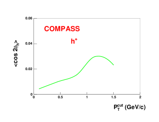
Figure 14: Predictions for $\langle\cos 2\phi_{h}\rangle$ corresponding to the production of positively charged hadrons as it will be measured by the COMPASS collaboration in the forthcoming future. The solid lines correspond to $\langle\cos 2\phi_{h}\rangle$ we find by including all orders in the $(k_{\perp}/Q)$ expansion. Notice that QCD corrections have no influence in this range of low $P_{T}$’s.

Fig. 12 shows our corresponding predictions for the SIDIS cross section – for the production of positively charged hadrons – as a function of the kinematical variables $z_{h}$, $x_{{}_{\!B\!j}}$, $y$ and $P_{T}$, as obtained from Eq. (3). Notice that we neglect nuclear corrections and use the isospin symmetry in order to obtain the parton distribution functions of the deuterium. Similarly to the HERMES case, the perturbative QCD corrections are negligible. Predictions for $\langle\cos\phi_{h}\rangle$ are presented in Fig. 13 and the higher-twist contributions to $\langle\cos 2\phi_{h}\rangle$ in Fig. 14. Similar results hold for negatively charged hadrons.

Finally, JLab collects and will collect data in the collisions of $6$ and $12$ GeV electrons from a fixed He³ target. In this case the relevant kinematical regions are the following:

$$Q^{2}>1\;({\rm GeV}/c)^{2}\quad W^{2}>4\;{\rm GeV}^{2}\quad P_{T}>0.1\;{\rm GeV}/c$$

$$1.0<E_{h}<3.5\;{\rm GeV}\quad\quad 0.4<z_{h}<0.7\quad\quad 0.1<x_{{}_{\!B\!j}}<0.6\quad\quad 0.4<y<0.85\>.$$ (26)

Our results for the corresponding SIDIS cross sections, $\langle\cos\phi_{h}\rangle$ and $\langle\cos 2\phi_{h}\rangle$ are shown in Figs. 15, 16 and 17 respectively: as for the previous experiments, also the JLab data are dominated by $\mathcal{O}(\alpha_{s}^{0})$ terms and are almost completely insensitive to the LO and NLO perturbative QCD corrections. Again, we show results for $\pi^{+}$ production, but very similar ones hold for $\pi^{-}$ and $\pi^{0}$, which we do not show.

All these results depend on intrinsic momenta, both $\mbox{\boldmath$k$}_{\perp}$ in the partonic distributions and $\mbox{\boldmath$p$}_{\perp}$ in the quark fragmentation. This is obvious for quantities like $d\sigma/dP_{T}$ and $\langle\cos\phi_{h}\rangle$ which could not even be defined, at $\mathcal{O}(\alpha_{s}^{0})$, without intrinsic motion (and pQCD corrections are negligible for the experiments we consider). However, this is also true for the differential cross-sections in $z$, $x_{{}_{\!B\!j}}$ and $y$: although they get contributions from intrinsic motion only at $\mathcal{O}(P_{T}/Q)^{2}$, as one can explicitly see from Eq. (6), these contributions can be sizeable in the kinematical domains of HERMES, COMPASS and JLab.

V Conclusions

We have considered the azimuthal and $P_{T}$ dependence of SIDIS data from low to large $P_{T}$; they both cannot be explained in the simple parton model ($\mathcal{O}(\alpha_{s}^{0})$) with collinear configurations. They can originate from intrinsic motions and/or pQCD corrections. The outcome of our analysis turns out to be very simple: up to $P_{T}\mathrel{\hbox to0.0pt{\lower 4.0pt\hbox{\hskip 1.0pt$\sim$}\hss}\raise 1.0pt\hbox{$<$}}1$ GeV/$c$ the simple parton model with unintegrated distribution and fragmentation functions explains the data and leads to a good evaluation of $\langle k_{\perp}\rangle$ and $\langle p_{\perp}\rangle$, while at larger $P_{T}$ values, $P_{T}\mathrel{\hbox to0.0pt{\lower 4.0pt\hbox{\hskip 1.0pt$\sim$}\hss}\raise 1.0pt\hbox{$>$}}1$ GeV/$c$, the perturbative QCD contributions originating from hard gluonic radiation processes and elementary scattering initiated by gluons, are dominant.

Having clearly established the complementarity of the two approaches, and in particular having gained full confidence in the domain of applicability of the unintegrated parton model, we have given predictions for the cross sections and for the values of $\langle\cos\phi_{h}\rangle$, as they will soon be measured by HERMES, COMPASS and JLab collaborations, mainly in the low $P_{T}$ region. These new data will be a very important tool to test our knowledge of the intrinsic partonic internal motion and on the TMD quark distribution and fragmentation functions.

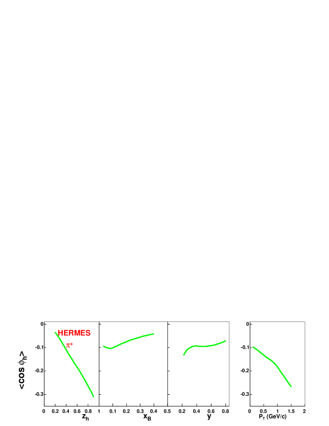
Figure 10: Predictions for $\langle\cos\phi_{h}\rangle$ corresponding to the production of $\pi^{+}$ as it will be measured by the HERMES collaboration in the forthcoming future. The solid lines correspond to $\langle\cos\phi_{h}\rangle$ we find by including all orders in the $(k_{\perp}/Q)$ expansion. Notice that QCD corrections have no influence in this range of low $P_{T}$’s.

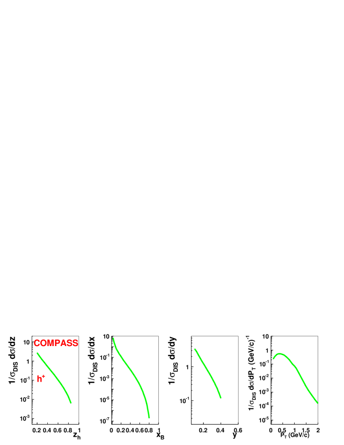
Figure 12: Predictions for the normalized SIDIS cross section corresponding to the production of positively charged hadrons as it will be measured by the COMPASS collaboration in the forthcoming future. The solid lines correspond to the SIDIS cross section as obtained by including all orders in the $(k_{\perp}/Q)$ expansion. Notice that QCD corrections have no influence in this range of low $P_{T}$’s.

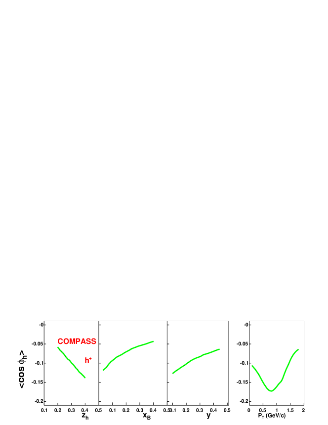
Figure 13: Predictions for $\langle\cos\phi_{h}\rangle$ corresponding to the production of positively charged hadrons as it will be measured by the COMPASS collaboration in the forthcoming future. The solid lines correspond to $\langle\cos\phi_{h}\rangle$ we find by including all orders in the $(k_{\perp}/Q)$ expansion. Notice that QCD corrections have no influence in this range of low $P_{T}$’s.

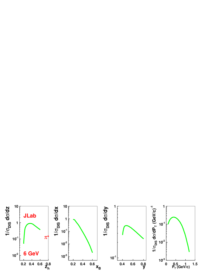
Figure 15: Predictions for the normalized SIDIS cross section corresponding to the production of $\pi^{+}$ as it will be measured by the JLab collaboration in the forthcoming future. The solid lines correspond to the SIDIS cross section as obtained by including all orders in the $(k_{\perp}/Q)$ expansion. Notice that QCD corrections have no influence in this range of low $P_{T}$’s.

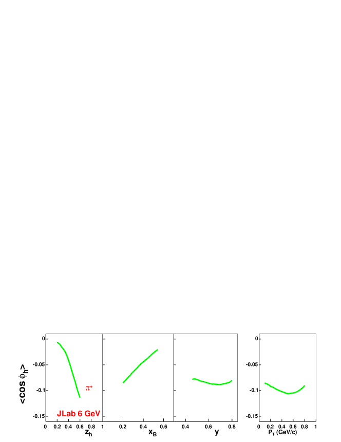
Figure 16: Predictions for $\langle\cos\phi_{h}\rangle$ corresponding to the production of $\pi^{+}$ as it will be measured by the JLab collaboration in the forthcoming future. The solid lines correspond to $\langle\cos\phi_{h}\rangle$ we find by including all orders in the $(k_{\perp}/Q)$ expansion. Notice that QCD corrections have no influence in this range of low $P_{T}$’s.

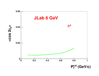
Figure 17: Predictions for $\langle\cos 2\phi_{h}\rangle$ corresponding to the production of $\pi^{+}$ as it will be measured by the JLab collaboration in the forthcoming future. The solid lines correspond to $\langle\cos 2\phi_{h}\rangle$ we find by including all orders in the $(k_{\perp}/Q)$ expansion. Notice that QCD corrections have no influence in this range of low $P_{T}$’s.

References

(1)
M. Anselmino, M. Boglione, U. D’Alesio, A. Kotzinian, F. Murgia, A. Prokudin,
Phys. Rev.D71 (2005) 074006.
(3)
HERMES Collaboration, A. Airapetian et al., Phys. Rev. Lett.94 (2005) 012002;
M. Diefenthaler (on behalf of the HERMES collaboration),
e-Print Archive: hep-ex/0507013.
(11)
H. Georgi and H. D. Politzer, Phys. Rev. Lett.40 (1978) 3.
(12)
A. Mendez, Nucl. Phys.B145 (1978) 199; A. Konig, P. Kroll, Z. Phys.C16 (1982) 89.
(13)
J. Chay, S.D. Ellis and W.J. Stirling, Phys. Rev.D45 (1992) 46.
(14)
B.A. Kniehl, G. Kramer, M. Maniatis, Nucl. Phys.B711 (2005) 345.
(15)
A. Daleo, D. de Florian and R. Sassot, Phys. Rev.D71 (2005) 034013.
(16)
X. Ji, J-W. Qiu, W. Vogelsang and F. Yuan, e-Print Archive: hep-ph/0602239; Phys. Rev.D73 (2006) 094017.
(17)
X. Ji, J-W. Qiu, W. Vogelsang and F. Yuan, Phys. Lett.B638 (2006) 178.
(18)
A.D. Martin, R.G. Roberts, W.J. Stirling and R.S. Thorne,
Phys. Lett.B531 (2002) 216
(19)
S. Kretzer, Phys. Rev.D62 (2000) 054001
(20) J. Ashman et al: EMC Collaboration, Z. Phys.C52 (1991) 361.
(21)
M. Derrick et al, ZEUS Collaboration, Z. Phys.C70 (1996) 1.
(22)
J. Breitweg et al, ZEUS Collaboration, Phys. Lett.B481 (2000) 199.
(23)
D. Boer and P.J. Mulders, Phys. Rev.D57 (1998) 5780.
(24)
J.C. Collins, Nucl. Phys.B396 (1993) 161.
(25)
V. Barone. Z. Lu and B-Q. Ma, Phys. Lett.B632 (2006) 277.