Implications of cosmic strings with time-varying tension
on CMB and large scale structure

Abstract

We investigate cosmological evolution and implications of cosmic strings with time-dependent tension. We derive basic equations of time development of the correlation length and the velocity of such strings, based on the one scale model. Then, we find that, in the case where the tension depends on some power of the cosmic time, cosmic strings with time-dependent tension goes into the scaling solution if the power is lower than a critical value. We also discuss cosmic microwave background anisotropy and matter power spectra produced by these strings. The constraints on their tensions from the Wilkinson microwave anisotropy probe (WMAP) three year data and Sloan digital sky survey (SDSS) data are also given.

I Introduction

Topological defects can be produced as a result of thermal Kibble or nonthermal KVY phase transitions at the symmetry breaking in the early universe. Among them, cosmic strings have been extensively investigated mainly because they could act as the seeds for large scale structure. Recent observations of the cosmic microwave background (CMB) anisotropy WMAP reveal that cosmic strings cannot be the primary source of primordial density fluctuations, and give the bound on the tension of cosmic strings $G\mu<2.7\times 10^{-7}$ at $95\%$ confidence level PWW , which is obtained by considering a hybrid scenario of adiabatic fluctuations generated during inflation plus isocurvature fluctuations produced by cosmic strings. The constraint given in other analysis such as Refs. Fraisse and Seljak are also in good agreement with theirs.

However, cosmic strings can still affect various astrophysics VSHK such as the early reionization ER , gravitational radiation GR , gravitational lensing effects GL , the neutrino masses BMY , and so on. Furthermore, an interesting possibility is revived that fundamental strings of the superstring theory can be expanded to cosmological sizes and act as cosmic strings CSS . In fact, F-strings and D-strings are produced at the end of brane inflation BI .

In almost all research so far, the tensions of cosmic strings have been assumed to be constant. Recently however, one of the authors (M.Y.) pointed out that tensions of cosmic strings can depend on the cosmic time MY . For example, a complex scalar field $\phi$, which allows a string solution, couples to another field $\chi$,

$$V(\phi,\chi)=\frac{\lambda}{4}(|\phi|^{2}-\chi^{2})^{2}+\frac{1}{2}m_{\chi}^{2}\chi^{2}.$$ (1)

When a coupling constant $\lambda$ is small enough, the backreaction to the oscillation of $\chi$ is negligible. Then, tension of a string $\mu$ is determined by the root mean square of the expectation value of $\chi$ and given by $\mu\propto a^{-3}$ ($a$:the scale factor), which is proportional to $t^{-3/2}$ in the radiation dominated era and $t^{-2}$ in the matter dominated era. Hence, the tension $\mu$ depends on the power of the cosmic time. Furthermore, in the warped geometry, the tension depends on the position of the brane in the bulk, which can depend on the cosmic time before the radion is fixed completely. Thus, it is quite natural to consider cosmic strings with time-dependent tension.

The key property of cosmological evolution of cosmic strings is scaling, which is confirmed by extensive investigations of cosmic strings with constant tension VSHK . It has been shown that the cosmic string network goes into the scaling regime, in which the typical length of the cosmic string network grows with the horizon scale. Then, the number of infinite strings per horizon volume is a constant irrespective of time and hence the ratio of the energy density of infinite strings to that of the background universe is constant. Thus, cosmic strings can generate scale invariant density fluctuations. Scaling property of the cosmic string network is confirmed both analytically Kibble and numerically AT ; BB ; AS by using the Nambu-Goto action NG , which can be obtained after integrating out heavy modes of particles and neglecting high curvature of the geometry.

As for cosmic strings with time-dependent tension, the followings are shown in Ref. MY . First of all, it is shown that the effective action of a cosmic string with time-dependent tension is given by the Nambu-Goto action with an additional factor for the time-dependent tension. By making use of such a Nambu-Goto-like action, the equation of motion in an expanding universe is derived and the evolution of cosmic strings with time-dependent tension is investigated. Then, it is confirmed that, in the case where the tension changes as the power $q$ of time, the string network goes into the scaling regime, in which the characteristic scale of the string network grows in proportion to the cosmic time. One should notice that the ratio of the energy density of infinite strings to that of the background universe is not necessarily constant due to the time dependence of the tension, different from the case of cosmic strings with constant tension. However, in Ref. MY , the constancy of string velocity is implicitly assumed to derive the scaling solution. In this paper, we also derive the equation of time development of string velocity based on the velocity-dependent one scale model MS and find a critical power of time dependence of the tension, below which the scaling property is realized and string velocity becomes almost constant.

When the tension of cosmic strings depends on time, its effects on astrophysics and cosmology can be significantly different from those of the conventional cosmic strings. Thus we should consider the implications of such cosmic strings on various astrophysical and cosmological issues. Among them, we study its effects on CMB and large scale structure in this paper. Since the time dependence of the tension strongly depends on models, we investigate it in some general settings. Here we assume the time dependence of the tension as $\mu\propto a^{n}$ and $\mu\propto\tau^{n}$ where $\tau$ is the conformal time and $n$ parametrize the dependence on the power. With this assumption, we study the CMB and matter power spectrum in models with the time dependent tension. For this purpose, we modified the CMBACT code developed and made publicly available by Pogosian and Vachaspati PV ; PWW to calculate the CMB anisotropy and the matter power spectrum induced by cosmic strings with time dependent tension. We will also give the constraint on the cosmic strings by comparing the predictions with recent cosmological observations, especially, the WMAP three-year data WMAP and the SDSS data SDSS . We would like to stress that these constraints are important in discussing astrophysical applications such as the early reionization, gravitational radiation, gravitational lensing effects, the neutrino masses, and so on.

This paper is organized as follows. In the next section, we derive basic equations to investigate cosmological evolution of cosmic strings with time-dependent tension and obtain the condition under which the string network goes into the scaling solution. In section III, we calculate the predictions of the CMB anisotropy and the matter power spectrum induced by cosmic strings with time-dependent tension and give the constraints on their tensions from the WMAP three year results and SDSS data. Since the time dependence of the tension strongly depends on a model, we concentrate on the case that the tension changes in proportion to the power of the conformal time or the scale factor. The final section is devoted to conclusions and discussion.

II Cosmological evolution of cosmic strings with time-dependent tension

As shown in Ref. MY , the effective action for a cosmic string with time-dependent tension is given by

$$S_{\rm eff}=-\int d^{2}\zeta\sqrt{-\gamma}\,\mu(\tau).$$ (2)

Here, two parameters $\zeta^{a}$($a=0,1$) characterize the worldsheet swept by a cosmic string with $x^{\mu}=x^{\mu}(\zeta^{a})$. We take the timelike coordinate $\zeta^{0}$ to be the cosmic conformal time $\tau$ and the spacelike coordinate $\zeta^{1}$ to be $\sigma$, which parametrizes the string at a fixed time. The metric is taken to be that of the spatially flat expanding universe,

$$ds^{2}=g_{\mu\nu}dx^{\mu}dx^{\nu}=dt^{2}-a^{2}(t)d\mbox{\boldmath${x}$}^{2}=a^{2}(\tau)(d\tau^{2}-d\mbox{\boldmath${x}$}^{2})$$ (3)

with $d\tau=dt/a(t)$. $\gamma_{ab}\equiv g_{\mu\nu}x^{\mu}_{,a}x^{\nu}_{,b}$ is the spacetime metric on the string worldsheet,

$$ds^{2} = g_{\mu\nu}dx^{\mu}dx^{\nu}$$ (4)

$$= \gamma_{ab}d\zeta^{a}d\zeta^{b}.$$

Here, the comma represents the partial derivative. Since we are interested only in the transverse motion of cosmic strings, the metric should satisfy the following condition,

$$\dot{\mbox{\boldmath${x}$}}\cdot\mbox{\boldmath${x}$}^{\prime}=0\quad\Longleftrightarrow\quad\gamma_{01}=\gamma_{10}=0,$$ (5)

where dots and primes represent derivatives with respect to conformal time $\tau$ and the spacelike parameter $\sigma$, respectively.

The Euler-Lagrange equation for the effective action is given by

$$\frac{\mu}{\sqrt{-\gamma}}\partial_{a}(\sqrt{-\gamma}\gamma^{ab}x^{\mu}_{b})+\mu^{,a}x^{\mu}_{,a}+\mu\Gamma^{\mu}_{\nu\sigma}\gamma^{ab}x^{\sigma}_{,a}x^{\nu}_{,b}=0,$$ (6)

where $\Gamma^{\mu}_{\nu\sigma}$ is the four-dimensional Christoffel symbol given by

$$\Gamma^{\mu}_{\nu\sigma}=\frac{1}{2}g^{\mu\tau}(g_{\nu\tau,\sigma}+g_{\tau\sigma,\nu}-g_{\nu\sigma,\tau}).$$ (7)

The time component of the equation of motion yields

$$\dot{\epsilon}+\frac{\dot{\mu}}{\mu}\epsilon+2\frac{\dot{a}}{a}\epsilon\mbox{\boldmath${x}$}^{2}=0$$ (8)

with $\epsilon\equiv\sqrt{\mbox{\boldmath${x}$}^{\prime\,2}/(1-\dot{\mbox{\boldmath${x}$}}^{2})}$. On the other hand, the spatial components yield

$$\ddot{\mbox{\boldmath${x}$}}+2\frac{\dot{a}}{a}(1-\dot{\mbox{\boldmath${x}$}}^{2})\dot{\mbox{\boldmath${x}$}}-\frac{1}{\epsilon}(\epsilon^{-1}\mbox{\boldmath${x}$}^{\prime})^{\prime}=0.$$ (9)

We define the energy $E$ of a cosmic string in an expanding universe as

$$E=a(\tau)\mu(\tau)\int d\sigma\epsilon.$$ (10)

The evolution of the energy density as $\rho\equiv E/V$ with $V$ some relevant volume is given by

$$\dot{\rho}=-2\frac{\dot{a}}{a}(1+\left\langle v^{2}\right\rangle)\rho,$$ (11)

where $\left\langle v^{2}\right\rangle$ is the average velocity squared of a cosmic string defined as

$$\left\langle v^{2}\right\rangle\equiv\left\langle\dot{\mbox{\boldmath${x}$}}^{2}\right\rangle\equiv\frac{\int d\sigma\epsilon\dot{\mbox{\boldmath${x}$}}^{2}}{\int d\sigma\epsilon}.$$ (12)

Note that multiplying the rate equation of $\rho$ by $d\tau/dt$ gives an equation with the same form but a derivative taken with respect to the cosmic time $t$.

The evolution of the string network is characterized by a correlation length $L$ as

$$\rho_{\infty}=\frac{\mu(t)}{L^{2}},$$ (13)

where $\rho_{\infty}$ is the energy density of a string whose length is larger than the horizon scale (called infinite strings). In fact, strings intercommute and their energy is transferred from infinite strings to loops. The rate of energy transfer from infinite strings to loops is given by

$$\dot{\rho}_{\infty\rightarrow{\rm loops}}=\tilde{c}v\frac{\rho_{\infty}}{L},$$ (14)

where $\tilde{c}$ parametrizes the efficiency of energy transfer and $v\equiv\sqrt{\left\langle v^{2}\right\rangle}$ is the average velocity. Then, the rate equation for the energy density of infinite strings becomes

$$\frac{d\rho_{\infty}}{dt}=-2H(1+v^{2})\rho_{\infty}-\tilde{c}v\frac{\rho_{\infty}}{L},$$ (15)

where $H$ is the Hubble parameter. Inserting Eq. (13) into this equation yields

$$\frac{dL}{dt}=HL(1+v^{2})+\frac{1}{2}\tilde{c}v+\frac{L}{2\mu}\frac{d\mu}{dt}.$$ (16)

On the other hand, the evolution equation of the velocity is given by

$$\frac{dv}{dt}=(1-v^{2})\left(\frac{\tilde{k}}{L}-2Hv\right).$$ (17)

Here we have taken $\left\langle\dot{\mbox{\boldmath${x}$}}^{2}\right\rangle^{2}=\left\langle\dot{\mbox{\boldmath${x}$}}^{4}\right\rangle$, which is exact up to second order terms. In the one-scale model, the typical curvature radius is given by the correlation length $L$,

$$\frac{a}{L}\hat{\mbox{\boldmath${u}$}}=\frac{d^{2}\mbox{\boldmath${x}$}}{ds^{2}},$$ (18)

where $\hat{\mbox{\boldmath${u}$}}$ is a unit vector and $s$ is the physical length along the string. As introduced in Ref. MS , we have defined the dimensionless parameter $\tilde{k}$, which is associated with the presence of small-scale structure,

$$\tilde{k}\equiv\frac{\left\langle(1-\dot{\mbox{\boldmath${x}$}}^{2})(\dot{\mbox{\boldmath${x}$}}\cdot\hat{\mbox{\boldmath${u}$}})\right\rangle}{v(1-v^{2})}.$$ (19)

Note that the velocity evolution equation (17) is the same as that for a string with constant tension because the terms related to time dependence of the tension are cancelled.

In order to investigate the time development of $L$, we define $\gamma$ as $L=\gamma t$ and assume that $\mu\propto t^{q}$. Then, Eqs. (16) and (17) can be recast into

$$\frac{1}{\gamma}\frac{d\gamma}{dt} = -\frac{1}{2t}\left(1-q-v^{2}-\frac{\tilde{c}v}{\gamma}\right),$$ (20)

$$\frac{dv}{dt} = \frac{1-v^{2}}{t}\left(\frac{\tilde{k}}{\gamma}-v\right),$$ (21)

where we have assumed the radiation domination. These equations have the stable fixed point $\gamma_{\rm r}$ and $v_{\rm r}$, which is given by

$$\gamma_{\rm r} = \frac{\tilde{c}_{\rm r}v_{\rm r}}{1-q-v^{2}_{\rm r}}=\sqrt{\frac{\tilde{k}_{\rm r}(\tilde{k}_{\rm r}+\tilde{c}_{\rm r})}{1-q}},$$ (22)

$$v_{\rm r} = \frac{\tilde{k}_{\rm r}}{\gamma_{\rm r}}=\sqrt{\frac{\tilde{k}_{\rm r}(1-q)}{\tilde{k}_{\rm r}+\tilde{c}_{\rm r}}}.$$ (23)

In the same way, the stable fixed point in a matter-dominated universe $\gamma_{\rm m}$ and $v_{\rm m}$ is given by

$$\gamma_{\rm m} = \frac{3\tilde{c}_{\rm m}v_{\rm m}}{2-3q-4v^{2}_{\rm m}}=\frac{3}{2}\sqrt{\frac{\tilde{k}_{\rm m}(\tilde{k}_{\rm m}+\tilde{c}_{\rm m})}{2-3q}},$$ (24)

$$v_{\rm m} = \frac{3\tilde{k}_{\rm m}}{4\gamma_{\rm m}}=\frac{1}{2}\sqrt{\frac{\tilde{k}_{\rm m}(2-3q)}{\tilde{k}_{\rm m}+\tilde{c}_{\rm m}}}.$$ (25)

Note that the stable fixed point exists only when $q<1$ in the radiation domination and $q<2/3$ in the matter domination. In case that the stable fixed point exists, the characteristic scale $L$ of a string network scales with time for strings with time-dependent tension. That is, the number of infinite strings per horizon volume is a constant irrespective of time. But it should be noted that, due to the time dependence of the tension, the ratio of the energy density of infinite strings to that of the background universe is not a constant.

It is convenient to work with the comoving correlation length $l\equiv L/a$ and the conformal time $\tau$. Then, the evolution equations are rewritten as

$$\dot{l} = \frac{\dot{a}}{a}lv^{2}+\frac{1}{2}\tilde{c}v+\frac{l}{2}\frac{\dot{\mu}}{\mu},$$ (26)

$$\dot{v} = (1-v^{2})\left(\frac{\tilde{k}}{l}-2\frac{\dot{a}}{a}v\right).$$ (27)

According to Ref. PV , we interpolate between these values through the radiation-matter transition,

$$\tilde{c}(\tau)=\frac{\tilde{c}_{r}+ga\tilde{c}_{m}}{1+ga},$$ (28)

$$\tilde{k}(\tau)=\frac{\tilde{k}_{r}+ga\tilde{k}_{m}}{1+ga},$$ (29)

where we take $\tilde{c}_{r}=0.23$, $\tilde{c}_{m}=0.18$, $\tilde{k}_{r}=0.17$, $\tilde{k}_{m}=0.49$, $g=300$ and $a(\tau)$ is normalized so that $a=1$ at present PV . Here, we expect that the time dependence of the tension has little effect on the parameters $\tilde{c}$ and $\tilde{k}$ because intercommutation is a local process near the string core and $\tilde{k}$ is a parameter associated with the presence of small-scale structure. For simplicity, we set the wiggleness parameter $\alpha$ to be unity.

III Constraints on the string tension

In this section, we first show CMB and matter power spectra seeded by cosmic strings whose tension varies with time in addition to those by the constant tension strings which are conventionally investigated. Then we discuss cosmological constraints on the tension. As is well known for the constant tension case, since they show no acoustic oscillation and positive correlation in temperature-polarization cross-correlation spectrum (TE), initial perturbation from cosmic strings alone cannot explain the observed CMB spectra and the inflationary adiabatic initial perturbation necessarily dominates. However, some contribution from cosmic string is still allowed. Therefore, we derive upper bounds on the string tension by studying how much the string contribution can be compared with the adiabatic one. We use the WMAP three-year data WMAP for CMB and SDSS data release 2 SDSS for galaxy clustering data to give the constraints. We denote the cosmological parameters as follows: baryon density $\omega_{b}$, matter density $\omega_{m}$, hubble parameter $h$, reionization optical depth $\tau$, spectral index of primordial spectrum $n_{s}$.

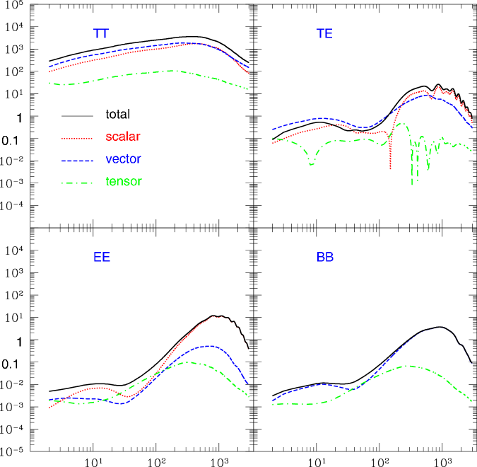
Figure 1: CMB power spectrum for the case with constant tension.

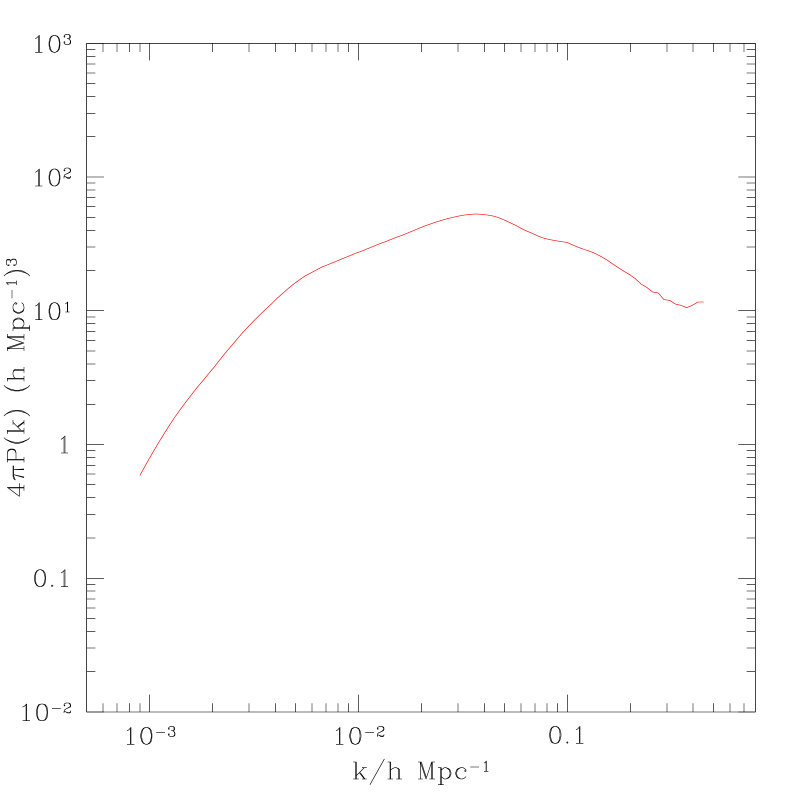
Figure 2: Matter power spectrum for the case with constant tension.

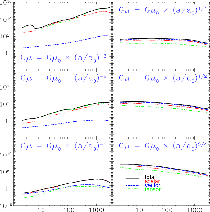
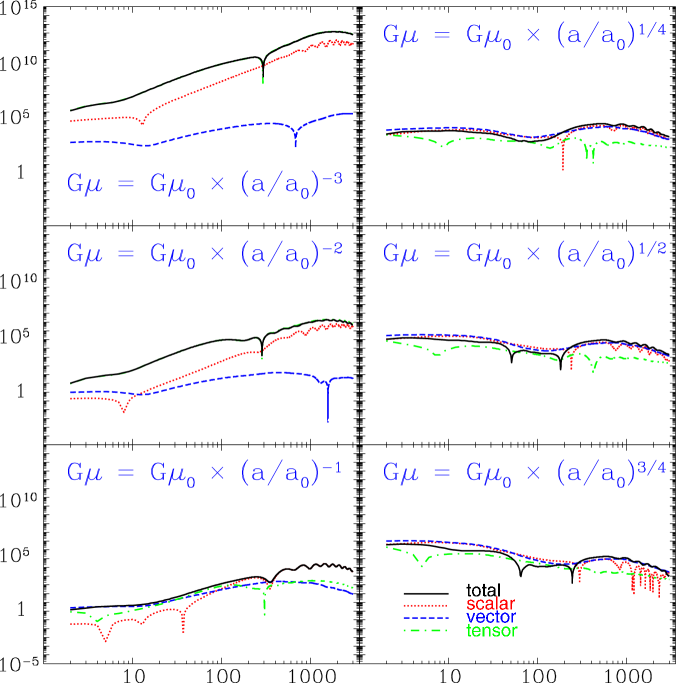
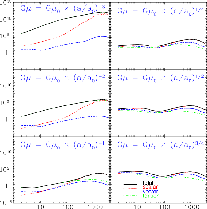
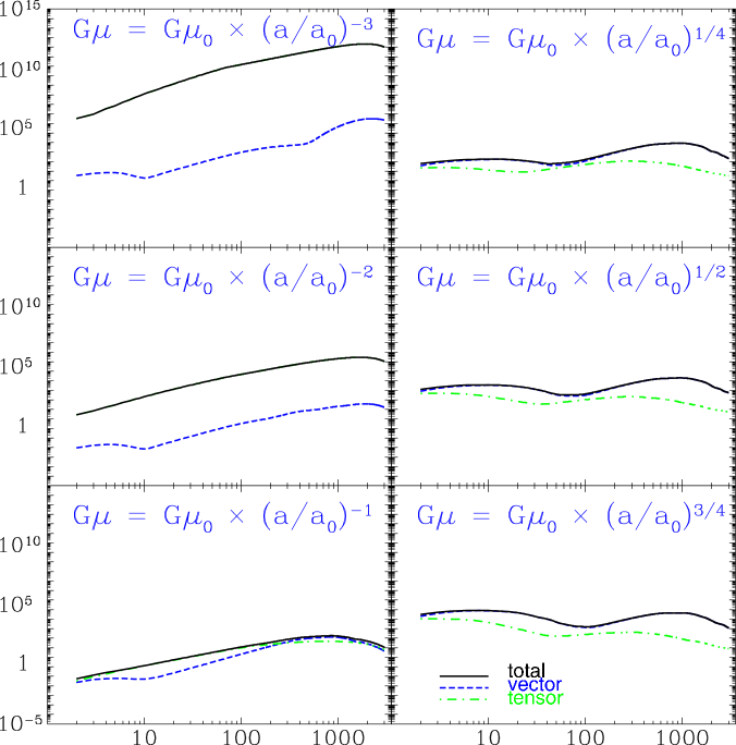
Figure 3: CMB TT, TE, EE, BB power spectra for the cases with time varying tension $G\mu\propto a^{n}$, $n=-3,-2,-1,1/4,1/2,3/4$. Scalar, vector, tensor modes and the total power spectrum are shown. Note that the absolute magnitude is given for TE power spectra.

Let us begin with showing the results of power spectra calculation of cosmic strings whose tension $\mu$ varies in proportion to some power $n$ of the scale factor $a$, $\mu\propto a^{n}$. For comparison, first we show the CMB and matter power spectra for the case with cosmic strings with constant tension in Figs. 1 and 2 respectively. Figure 3 and 5 are for the cases with time dependent tension with negative powers ($n=-3,-2,-1$) and with positive powers ($n=1/4,1/2,3/4$). Note that, as shown above, the string network does not follow a scaling law for $n\gtrsim 1$. These spectra are calculated by modifying CMBACT code PV ; PWW which is based on CMBFAST code Seljak:1996is . In these figures, the cosmological parameters are taken to be the WMAP mean values $\omega_{b}=0.0223$, $\omega_{m}=0.127$, $h=0.73$, $\tau=0.09$ WMAP .

We use these spectra sourced by cosmic strings to place upper bound on the string tension. After adding power spectra from adiabatic initial perturbation, we plug the sum into the likelihood codes for CMB and galaxy clustering supplied respectively by the WMAP group Jarosik:2006ib ; Hinshaw:2006ia ; Page:2006hz and the SDSS group SDSS . For each value of the string tension, we calculate $\chi^{2}$ by marginalizing over the amplitude of adiabatic power spectrum and the bias factor between observed galaxy power spectrum and theoretical matter power spectrum (the sum of adiabatic and string contribution). In connection with the latter, we use the galaxy clustering measurements in 19 $k$-bands with $k<0.2h/$Mpc and assume that the bias factor does not depend on $k$. Other cosmological parameters are fixed to be $\omega_{b}=0.0221$, $\omega_{m}=0.127$, $h=0.725$, $\tau=0.0913$, $n_{s}=0.957$ for deriving WMAP alone constraints and $\omega_{b}=0.0225$, $\omega_{m}=0.145$, $h=0.664$, $\tau=0.0816$ and $n_{s}=0.959$ for WMAP plus SDSS constraints, which minimize $\chi^{2}$ of respective data sets when the cosmic string contribution is absent ($i.e.$ when only adiabatic initial perturbation exists). This minimization is carried out by the method introduced in Ref. Ichikawa:2004zi and the minimum $\chi^{2}$ for WMAP alone case agrees with the WMAP analysis as noted in Ref. Fukugita:2006rm . We show the values of $\Delta\chi^{2}$ as a function of $G\mu$ at the present time for some cases in Fig. 7. In table 1, we report upper bounds at 95% confidence level by reading $G\mu$ which gives $\Delta\chi^{2}=4$. While the bounds on string tensions at present become stringent for negative powers, they are weakened for positive powers. The inclusion of the SDSS data does not improve the constraints significantly.

Note that our omission of full marginalization over the cosmological parameters might underestimate upper bounds, but we note that we have obtained the constraint from WMAP and SDSS for the constant tension case to be $G\mu<1.6\times 10^{-7}$ in good agreement with the bound $G\mu<2.7\times 10^{-7}$ obtained by Pogosian, Wasserman and Wyman PWW . Our result for the case with constant tension also agrees with those obtained in Refs. Fraisse and Seljak . This shows that our rather simplified way of estimating the bounds works well.

We repeat similar analysis with the cosmic strings whose tension scales as a power law of the conformal time $\tau$, $\mu\propto\tau^{n}$. The power spectra are shown in figures 4 and 6, and constraints are summarized in table 2. We have obtained constraints which show similar trend to the case of a power law of $a$. They become significantly severer for the cases of negative powers.

IV Conclusions and Discussion

In this paper, we have discussed cosmological evolution and implications of cosmic strings with time-dependent tension. First of all, we have derived equations of motions based on the velocity-dependent one scale model in the expanding universe. By using these equations, we investigate whether cosmic strings with time-dependent tension go into the scaling solution when the tension depends on some power of the cosmic time $\mu\propto t^{q}$. Then, we find that such strings relax into the scaling solution only when $q<1$ in the radiation domination and $q<2/3$ in the matter domination.

Then we showed the CMB and matter power spectra sourced by cosmic strings with time-dependent tension. As shown in the previous section, the spectra can be different significantly from those produced by the conventional cosmic strings with constant tension. We have also discussed the constraints on the time-dependent tension from the Wilkinson microwave anisotropy probe (WMAP) three year data and Sloan digital sky survey (SDSS) data. Since the time dependence of the tension strongly depends on models, here we considered it in some general settings. For the time dependence of string tensions, we assumed that the tension $\mu$ changes as some power of the scale factor $a$, $\mu\propto a^{n}$, and the conformal time $\tau$, $\mu\propto\tau^{n}$. The constraints on $\mu$ for various values of $n$ were given. For the cases with negative powers, the bounds on string tensions at present time become much stronger than those for the case with constant tension. One should, however, notice that the tension can be large in the past in this case, which may have implications on the structure formation at very small scales. On the other hand, the bounds are weakened for positive powers, which may lead to large amount of gravitational radiation background. We will explorer these possibilities in future work.

Tables:

$n$	WMAP alone (95%)	WMAP+SDSS (95%)
-3	$5.5\times 10^{-24}$	$5.5\times 10^{-24}$
-2	$2.8\times 10^{-16}$	$2.9\times 10^{-16}$
-1	$3.7\times 10^{-11}$	$3.8\times 10^{-11}$
0	$1.7\times 10^{-7}$	$1.6\times 10^{-7}$
1/4	$6.4\times 10^{-7}$	$5.8\times 10^{-7}$
1/2	$1.4\times 10^{-6}$	$1.2\times 10^{-6}$
3/4	$3.0\times 10^{-6}$	$2.7\times 10^{-6}$

Table 1: Constraints for constant and time varying ($G\mu\propto a^{n}$, $n=-3,-2,-1,0,1/4,1/2,3/4$) tension. We quote the upper bounds on $G\mu$ at the present epoch ($a=1$).

$n$	WMAP alone (95%)	WMAP+SDSS (95%)
-3	$1.8\times 10^{-19}$	$1.8\times 10^{-19}$
-2	$2.9\times 10^{-13}$	$3.0\times 10^{-13}$
-1	$1.1\times 10^{-9}$	$1.1\times 10^{-9}$
0	$1.7\times 10^{-7}$	$1.6\times 10^{-7}$
1/4	$4.0\times 10^{-7}$	$3.8\times 10^{-7}$
1/2	$6.3\times 10^{-7}$	$5.6\times 10^{-7}$
3/4	$9.0\times 10^{-7}$	$8.2\times 10^{-7}$

Table 2: Constraints for constant and time varying ($G\mu\propto\tau^{n}$, $n=-3,-2,-1,0,1/4,1/2,3/4$) tension. We quote the upper bounds on $G\mu$ at the present epoch ($\tau=1.5\times 10^{4}$).

Figures:

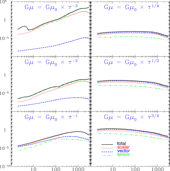
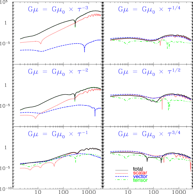
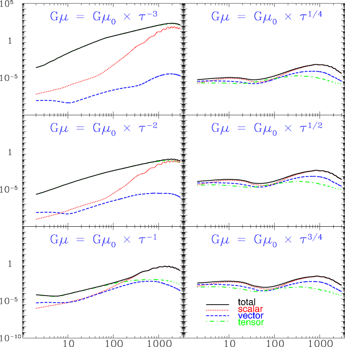
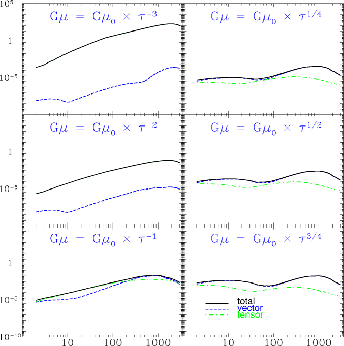
Figure 4: CMB TT, TE, EE, BB power spectra for the cases with time varying tension $G\mu\propto\tau^{n}$, $n=-3,-2,-1,1/4,1/2,3/4$. Scalar, vector, tensor modes and the total power spectrum are shown. Note that the absolute magnitude is given for TE power spectra.

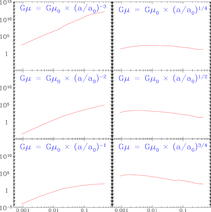
Figure 5: Matter power spectra for the cases with time varying tension $G\mu\propto a^{n}$, $n=-3,-2,-1,1/4,1/2,3/4$.

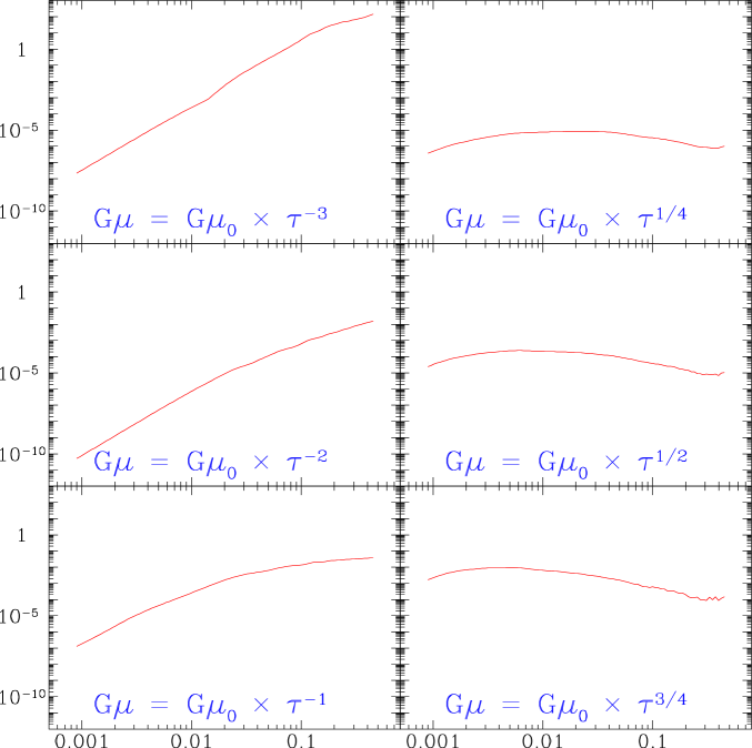
Figure 6: Matter power spectra for the cases with time varying tension $G\mu\propto\tau^{n}$, $n=-3,-2,-1,1/4,1/2,3/4$.

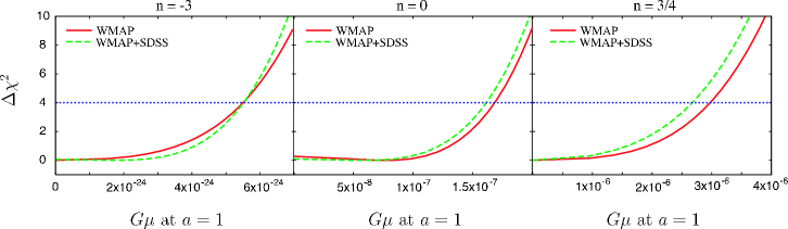
Figure 7: The values of $\Delta\chi^{2}$ from WMAP only and WMAP+SDSS are shown as a function of $G\mu$ at the present time. Here we assume the time dependence of $G\mu$ as $G\mu\propto a^{n}$. The cases with $n=-3,0$ and $3/4$ are shown.

References

- (1)
- (2) T. W. B. Kibble, J. Phys. A 9, 1387 (1976).
- (3) L. A. Kofman and A. D. Linde, Nucl. Phys. B282, 555 (1987); Q. Shafi and A. Vilenkin, Phys. Rev. D 29, 1870 (1984); E. T. Vishniac, K. A. Olive, and D. Seckel, Nucl. Phys. B289, 717 (1987); J. Yokoyama, Phys. Lett. B 212, 273 (1988); Phys. Rev. Lett. 63, 712 (1989).
- (4) C. L. Bennett et al., Astrophys. J. Suppl. 148, L1 (2003); D. N. Spergel et al., astro-ph/0603449.
- (5) L. Pogosian, S. -H. H. Tye, I. Wasserman and M. Wyman, Phys. Rev. D 68, 023506 (2003); L. Pogosian, M. Wyman, and I. Wasserman, J. Cosmol. Astropart. Phys. 09, 008 (2004); M. Wyman, L. Pogosian, and I. Wasserman, Phys. Rev. D 72, 023513 (2005); 73, 089905 (2006); L. Pogosian, M. Wyman, and I. Wasserman, astro-ph/0604141.
- (6) A. A. Fraisse, astro-ph/0503402.
- (7) U. Seljak, A. Slosar and P. McDonald, arXiv:astro-ph/0604335.
- (8) For review, see A. Vilenkin and E. P. S. Shellard, Cosmic String and Other Topological Defects (Cambridge University Press, Cambridge, England, 1994); M. B. Hindmarsh and T. W. B. Kibble, Rep. Prog. Phys. 58, 477 (1995).
- (9) P. P. Avelino and A. R. Liddle, Mon. Not. R. Astron. Soc. 348, 105 (2004); P. P. Avelino and D. Barbosa, Phys. Rev. D 70, 067302 (2004); L. Pogosian and A. Vilenkin, Phys. Rev. D 70, 063523 (2004); K. D. Olum and A. Vilenkin; astro-ph/0605465.
- (10) A. Vilenkin, Phys. Lett. 107B, 47 (1981); T. Damour and A. Vilenkin, Phys. Rev. D 71, 063510 (2005).
- (11) M. Sazhin et al., Mon. Not. R. Astron. Soc. 343, 353 (2003); R. Schild et al., Astron. Astrophys. 422, 477 (2004).
- (12) R. H. Brandenberger, A. Mazumdar, and M. Yamaguchi, Phys. Rev. D 69, 081301(R) (2004).
- (13) E. Witten, Phys. Lett. 153B, 243 (1985).
- (14) N. Jones, H. Stoica, and S. -H. H. Tye, J. High Energy Phys. 07, 051 (2002); S. Sarangi and S. -H. H. Tye, Phys. Lett. B 536, 185 (2002); N. T. Jones, H. Stoica, S. -H. H. Tye, Phys. Lett. B 563, 6 (2003).
- (15) M. Yamaguchi, Phys. Rev. D 72, 043533 (2005).
- (16) A. Albrecht and N. Turok, Phys. Rev. Lett. 54, 1868 (1985); A. Albrecht and N. Turok, Phys. Rev. D 40, 973 (1989).
- (17) D. P. Bennett and F. R. Bouchet, Phys. Rev. Lett. 60, 257 (1988); 63, 2776 (1989); Phys. Rev. D 41, 2408 (1990).
- (18) B. Allen and E. P. S. Shellard, Phys. Rev. Lett. 64, 119 (1990).
- (19) Y. Nambu, in Proceedings of International Conference on Symmetries & Quark Models Lectures at the Copenhagen Summary Symposium, 1970; T. Goto, Prog. Theor. Phys. 46, 1560 (1971).
- (20) M. Yamaguchi, J. Yokoyama, M. Kawasaki, Prog. Theor. Phys. 100, 535 (1998); M. Yamaguchi, M. Kawasaki, and J. Yokoyama, Phys. Rev. Lett. 82, 4578 (1999); M. Yamaguchi, Phys. Rev. D 60, 103511 (1999); M. Yamaguchi, J. Yokoyama, and M. Kawasaki, ibid. 61, 061301(R) (2000); M. Yamaguchi and J. Yokoyama, ibid. 66, 121303(R) (2002);67, 103514 (2003).
- (21) M. Barriola and A. Vilenkin, Phys. Rev. Lett. 63, 341 (1989); D. P. Bennett and S. H. Rhie, ibid. 65, 1709 (1990); U. Pen, D. N. Spergel, and N. Turok, Phys. Rev. D 49, 692 (1994); M. Yamaguchi, Phys. Rev. D 64, 081301(R) (2001); 65, 063518 (2002).
- (22) C. J. A. P. Martins and E. P. S. Shellard, Phys. Rev. D 53, 575(R) (1996); 54, 2535 (1996).
- (23) M Tegmark et al., Astrophys. J. 606, 702 (2004).
- (24) L. Pogosian and T. Vachaspati, Phys. Rev. D 60, 083504 (1999).
- (25) U. Seljak and M. Zaldarriaga, Astrophys. J. 469, 437 (1996)
- (26) N. Jarosik et al., arXiv:astro-ph/0603452.
- (27) G. Hinshaw et al., arXiv:astro-ph/0603451.
- (28) L. Page et al., arXiv:astro-ph/0603450.
- (29) K. Ichikawa, M. Fukugita and M. Kawasaki, Phys. Rev. D 71, 043001 (2005).
- (30) M. Fukugita, K. Ichikawa, M. Kawasaki and O. Lahav, arXiv:astro-ph/0605362.