The $Q_{t}$ distribution of the Breit current hemisphere in DIS as a probe of small-$x$ broadening effects

Abstract:

We study the distribution $1/\sigma\,d\sigma/dQ_{t}$, where $Q_{t}$ is the modulus of the transverse momentum vector, obtained by summing over all hadrons, in the current hemisphere of the DIS Breit frame. We resum the large logarithms in the small $Q_{t}$ region, to next-to–leading logarithmic accuracy, including the non-global logarithms involved. We point out that this observable is simply related to the Drell-Yan vector boson and predicted Higgs $Q_{t}$ spectra at hadron colliders. Comparing our predictions to existing HERA data thus ought to be a valuable source of information on the role or absence of small-$x$ (BFKL) effects, neglected in conventional resummations of such quantities.

1 Introduction

With the imminent advent of the LHC, considerable effort is being dedicated to utilising existing collider data and theoretical predictions for QCD observables to foster an even better knowledge of crucial parameters such as the strong coupling constant and parton distributions in hadrons [1].

An invaluable source for such data is the HERA collider, which continues to play an important role in phenomenological studies of QCD. The recently concluded HERA-LHC workshop was in fact dedicated towards the aim of directly linking HERA QCD studies to those that will be important in a discovery context at the LHC.

In the present paper we shall highlight one such study. To illustrate our point we choose the transverse momentum ($Q_{t}$) spectrum of the Higgs boson for which very accurate theoretical predictions exist in the literature [2]. These estimates resum large logarithms in the small $Q_{t}$ limit to next-to–next-to leading logarithmic (NNLL) accuracy. The resummed predictions are then combined with fixed next-to–leading order (NLO) computations [3] so as to achieve the best possible accuracy over a wide range of $Q_{t}$. Such accurate studies are important in the context of formulating improved strategies to extract the signal and to enhance its statistical significance over backgrounds.

One concern that has been a point for some discussion (see e.g. Ref. [4]) is the role that might be played by neglected small-$x$ effects that one may expect could be relevant at the $x$ values involved in vector boson and Higgs production at the LHC. Here $x$ can be interpreted, as usual, as the momentum fraction of the incoming hadron carried by the struck parton. If neglected small-$x$ effects are indeed important in this context, they could in principle lead to broader $Q_{t}$ spectra than those predicted by conventional resummations (sometimes also referred to as Collins-Soper–Sterman or CSS formalism [5]) alone. Henceforth we shall refer to these resummations involving $Q_{t}$ spectra in hadron–hadron collisions with the generic label Drell-Yan $Q_{t}$ resummations.

It was observed for instance in Ref. [4] that effects due to small-$x$ enhancements that were suggested by phenomenological studies [6] for semi-inclusive DIS (SIDIS) $Q_{t}$ distributions, could be very significant (especially in the context of massive vector-boson production) when extrapolated to the smaller $x$ values that will be important at the LHC. It was also suggested in Ref. [4] that such effects could be visible with Tevatron (run 2) data if one concentrates on forward production of vector bosons alone rather than integrating over all rapidities. On the other hand, studies for many event-shape variables in the current hemisphere of the Breit frame in DIS have been very successful, down to moderately small $x$ values ($x\approx 10^{-2}$), based on resummation [7, 8, 9] that did not account for BFKL or formal small-$x$ effects. The comparison to HERA data for several event-shape variables can be found in [9].

It is also clear however that event-shapes are somewhat different from $Q_{t}$ spectra of the Drell-Yan type, significantly due to their direct sensitivity to gluon emission, rather than purely through recoil. This difference means that event-shape variables receive non-perturbative corrections that scale as $1/Q$ [10], where $Q$ is the DIS hard scale. These power corrections are due to soft gluon emission alone and hence are independent of $x$. The quantity we shall study in the present article is closer in nature to the Drell-Yan $Q_{t}$ spectra since the leading non-perturbative effects here scale as $1/Q^{2}$ and can be associated to what is commonly known as “intrinsic $k_{t}$” of partons inside hadrons. Thus one would expect any missing small-$x$ effects that appear in the present context (perhaps as suggested in Ref. [4] in terms of a small-$x$ enhanced smearing of the conventional resummation), to manifest themselves in a very similar way in the Drell-Yan case. It is thus conceivable that for the $Q_{t}$ distribution we present here, deviations are seen from the resummed form, even at $x$ values already studied successfully for event-shape variables.

To be more precise, the observable we study here is the distribution $1/\sigma\,d\sigma/dQ_{t}$, with $Q_{t}$ being the modulus of the transverse momentum vector of all particles in the current hemisphere (${\mathcal{H}_{c}}$) of the DIS Breit frame:

$$\vec{Q}_{t}=\sum_{i\in{\mathcal{H}_{c}}}\vec{k}_{t,i}\,,$$ (1)

where $\vec{k}_{t}$ is measured with respect to the photon axis. Note that the addition over particles mentioned above, is vectorial in nature, in contrast to say that involved in event-shapes like the jet broadening observable [7], where one adds the modulii of individual particle transverse momenta. This is also a different quantity from the resummed $z$ flow studied in Refs. [4, 6] while also being directly related to the Drell-Yan $Q_{t}$ spectra and thus should provide an independent probe of small-$x$ broadening effects.

To relate the quantity here to $Q_{t}$ spectra in Drell-Yan type processes one notes that in the Drell-Yan case one has the massive vector-boson recoiling against emissions from two incoming hard partons, while for our DIS example, the transverse momentum of the current hemisphere is equal and opposite to that of the remnant hemisphere. If one assumes the remnant hemisphere $Q_{t}$ spectrum to be entirely generated by emissions from a single incoming leg the relationship to Drell-Yan $Q_{t}$ is obvious: we just have to account for the form-factor of one incoming parton instead of two and thus we have, at the level of form-factors, $\Delta^{N}_{\mathrm{DIS}}(Q,Q_{t})=\sqrt{\Delta^{N}_{\mathrm{DY}}(Q,Q_{t})}$. The variable $N$ indicates moment space, conjugate to $x$.

The simple relationship we mentioned immediately above breaks down at the next-to–leading logarithmic (NLL) level, due to the non-global nature [11, 12] of the DIS observable we have introduced. Non-globalness in the present case is a consequence of looking at just a single hemisphere and provides an extra factor in the DIS case, to do with soft emissions at large angles, which is absent for the global Drell-Yan quantity. We shall of course account for this factor, but we stress here that the fundamental relationship of our quantity to Drell-Yan $Q_{t}$ (which is exactly of the square-root form we wrote above, at leading-logarithmic accuracy) is unchanged by this complication. In particular any neglect of terms that are enhanced at small $x$, ought to be of similar significance in the two cases.

To further this investigation we obtain here a resummed result for the above quantity, to next-to–leading logarithmic (NLL) accuracy and combine it with fixed-order predictions to $\mathcal{O}(\alpha_{s}^{2})$ accuracy. Our result is thus suitable for comparison with data over the entire measured range of $Q_{t}$ values. We also comment on the effect of smearing our result with a Gaussian function, as is usual to accommodate the so-called intrinsic $k_{t}$ of the incoming parton, which has a non-perturbative origin. The resultant prediction can then be directly compared to data which should be of interest especially at lower $x$ values. If discrepancies are visible at low $x$ then one may consider a small-$x$ enhanced smearing function as was the case in Refs. [4, 6]. This is certainly not a substitute for a detailed treatment based on a physical understanding of the small-$x$ region but merely a phenomenological investigation into how such effects may be parameterised if present in the first place. Subsequently one may also consider the extrapolation of our findings to hadron colliders. We note that preliminary data from H1 are already available [13] and await the final versions together with potential data from the ZEUS collaboration.

The outline of this paper is as follows: in section 2 we put together the different ingredients required to obtain our NLL resummed result which we compute in impact parameter or $b$ space as is most convenient for $Q_{t}$ resummations. Once we obtain the $b$ space answer we find, in the 3following section, its transform to $Q_{t}$ space and comment on its main features. In section 4 we carry out the matching of our resummed result to the full ${\mathcal{O}}\left(\alpha_{s}^{2}\right)$ result from the fixed-order program DISENT [14]. 5Finally we comment on the potential role of non-perturbative effects that are expected to take the form of a smearing of the $Q_{t}$ distribution with a function representing the “intrinsic transverse momentum” of partons inside hadrons. Here one may try different choices for the smearing function and search for any discrepancies at lower $x$ values, between our results and the data. We shall leave the details of this to our forthcoming phenomenological investigation [15].

2 Resummation

At Born level, the struck quark is aligned along the photon axis, the quantity in question ($Q_{t}$) vanishes and the distribution is essentially a delta function: $d\sigma/dQ_{t}\sim\delta(Q_{t})$.

At small $Q_{t}$ the emission of soft and collinear gluons deform the delta function. One may, on general grounds, expect this deformation to take the form of a Sudakov form-factor. This is essentially true over a large range of $Q_{t}$ values with the caveat that at very small $Q_{t}$, the correct result is no longer of Sudakov form. The reason for this is the Parisi-Petronzio observation that the smallest $Q_{t}$ values are in fact obtained by vectorial cancellation of emissions rather than by suppressing the transverse momenta of each individual emission [16]. We shall explain this issue more quantitatively, with reference to our observable, in a later 3section. For now we proceed with resumming the large logarithms that arise at small $Q_{t}$.

To carry out the resummation, we have to address two distinct kinematic regimes:

• collinear emissions (soft or hard) along the directions of the incoming and scattered quark directions.

• soft emissions at large angles to the incoming and scattered (outgoing) quark axis (since in the Breit frame the incoming and scattered quarks are back-to–back at Born level). This contribution arises due to the non-global nature [11, 12] of the observable and is a correlated multi-gluon emission term, that can only be computed in the large $N_{c}$ limit.

We shall treat each region in turn starting with the collinear enhanced contribution and then including the non-global term that arises from the piece of the fixed-order matrix elements with only soft enhancement (i.e. is integrable over soft gluon directions).

2.1 Pure collinear contribution

The collinear contribution is simple to assess since one can, to the NLL accuracy we seek, consider collinear radiation as being included in the evolution of the incoming and outgoing hard quark jets. In order to derive the NLL pure collinear contribution it proves useful to first consider the observable as defined in Eq. (1). Since one is dealing with soft and/or collinear gluon emission alone, we are looking at a tiny deviation from the Born configuration. Thus the sum over current hemisphere emissions, on the RHS of Eq. (1), includes a contribution from the transverse momentum of the outgoing current quark. To work in terms of secondary emissions alone, one uses conservation of transverse momentum to write Eq. (1) as:

$$\vec{Q}_{t}=-\sum_{i\in{\mathcal{H}_{R}}}\vec{k}_{t,i}\,,$$ (2)

where the sum now runs over all final-state particles in the remnant hemisphere. In the collinear region there is an important simplification, in that all these emissions can, to our accuracy, be attributed to the showering of the incoming quark. Note that since one is now inclusive over current-hemisphere emissions, we can neglect the collinear evolution of the outgoing quark. This will correct our resummed result by a factor of relative order $\alpha_{s}$, but not enter into the NLL form-factor we aim to compute.

The next step is to consider multiple collinear gluon branchings on the incoming hard leg. In this region the squared matrix-element can be approximated to NLL accuracy by a product in $N$ space of individual gluon emissions from the hard incoming quark, where $N$ is the moment variable conjugate to Bjorken $x$. Taking first just soft and collinear emissions, where we can just as well work in $x$ space, one can write:

$$\frac{1}{\sigma_{0}}\frac{d\sigma}{dQ_{t}^{2}}\approx\sum_{n}\int dP_{n}\,\delta(p_{t}^{2}-Q_{t}^{2})\,d^{2}\vec{p}_{t}\,\delta^{2}\left(\vec{p}_{t}+\sum_{i\in\mathcal{H}_{R}}^{n}\vec{k}_{t,i}\right),$$ (3)

where $dP_{n}$ is the differential $n$ gluon emission probability and we introduced the vector $\vec{p}_{t}$, which is the vectorial sum of transverse momenta of particles in $\mathcal{H}_{R}$. Note that for purely soft and collinear emissions the parton distribution function (pdf) cancels with that in $\sigma_{0}$, the Born cross-section. This is not correct in the hard-collinear region and we will re-introduce the pdf while considering those emissions. For the final result, we shall also normalise to the cross-section including up to ${\mathcal{O}}(\alpha_{s}^{2})$ corrections, rather than merely the Born cross-section.

We first compute the integrated quantity:

$$\frac{1}{\sigma_{0}}\sigma(Q,Q_{t})=\frac{1}{\sigma_{0}}\int_{0}^{Q_{t}^{2}}\frac{d\sigma}{dQ_{t}^{\prime 2}}dQ_{t}^{\prime 2}\approx\sum_{n}\int dP_{n}\,\theta(Q_{t}-p_{t})\,d^{2}\vec{p}_{t}\,\delta^{2}\left(\vec{p}_{t}+\sum_{i\in\mathcal{H}_{R}}\vec{k}_{t,i}\right).$$ (4)

One can then express:

$$\delta^{2}\left(\vec{p}_{t}+\sum_{i\in\mathcal{H}_{R}}{\vec{k}_{t,i}}\right)=\int\frac{d^{2}\vec{b}}{(2\pi)^{2}}e^{i\vec{b}.\vec{p}_{t}}\prod_{i\in\mathcal{H}_{R}}e^{i\vec{b}.\vec{k}_{t,i}}\,.$$ (5)

Having achieved our aim of factorising the delta function constraint into a product of individual gluon contributions, we integrate over $\vec{p}_{t}$ which reduces the above to:

$$\frac{1}{\sigma_{0}}\sigma(Q,Q_{t})\approx\sum_{n}\int dP_{n}\,Q_{t}\,J_{1}(b\,Q_{t})\,db\prod_{i\in\mathcal{H}_{R}}e^{i\vec{b}.\vec{k}_{t,i}}\,,$$ (6)

where in writing the above we made use of $\int_{0}^{2\pi}d\theta\,\exp\left(i\,b\,p_{t}\cos\theta\right)=2\pi J_{0}(b\,p_{t})$, and $uJ_{1}(u)=\int_{0}^{u}u^{\prime}J_{0}(u^{\prime})du^{\prime}$ with $J_{0}$ and $J_{1}$ being the zeroth and first order Bessel functions.

The emission probability $dP_{n}$ factorises for soft and collinear emissions into an essentially classical independent-emission pattern:

$$dP_{n}=\frac{1}{n!}\prod_{i\in\mathcal{H}_{R}}C_{F}\frac{\alpha_{s}(k_{t,i}^{2})}{\pi}\frac{d^{2}\vec{k}_{t,i}}{\pi k_{t,i}^{2}}d\eta_{i}\,,$$ (7)

where $\vec{k}_{t,i}$ and $\eta_{i}$ refer to the transverse momenta and rapidity of the $i^{\textrm{th}}$ emission with respect to the incoming quark direction . Since the incoming quark is anti-parallel to the photon axis, in the Breit frame, the $k_{t}$ immediately above is the same to NLL accuracy as that measured with respect to the photon axis and we do not distinguish the two. The coupling $\alpha_{s}$ is defined in the CMW scheme [17]. We note that the rapidity integration is bounded by $\eta=0$ at large angles to the incoming quark since we are considering emissions in the remnant hemisphere alone.

Summing over all emissions in the remnant hemisphere using the factorised forms (5) and (7) and inserting virtual corrections according to the emission pattern (7) (with an additional factor $(-1)^{n}$) we arrive at the resummed soft and collinear contribution to $\sigma(Q,Q_{t})/\sigma_{0}$:

$$\int Q_{t}\,J_{1}(b\,Q_{t})\,\exp[-R_{\mathrm{sc}}(b)]\,db\,,$$ (8)

where $R_{\mathrm{sc}}(b)$ is the “radiator” accounting for soft and collinear emissions by the incoming quark:

$$R_{\mathrm{sc}}(b)=-\frac{C_{F}}{\pi}\int\frac{d^{2}\vec{k}_{t}}{\pi k_{t}^{2}}\,d\eta\,\alpha_{s}(k_{t}^{2})\,\left(e^{i\vec{b}.\vec{k}_{t}}-1\right).$$ (9)

We remind the reader that one needs to correct the above expression to obtain single-logarithms arising from hard collinear radiation as well as those that arise in the large-angle region from soft emissions, which we shall do presently.

Let us for the moment concentrate on the quantity $R_{\mathrm{sc}}(b)$, which is the most important piece of the result since it contains the leading (double) logarithms. Integrating over the polar angle variable in Eq. (9) we obtain:

$$R_{\mathrm{sc}}(b)=-\frac{2C_{F}}{\pi}\int\frac{dk_{t}}{k_{t}}d\eta\,\alpha_{s}(k_{t}^{2})\left(J_{0}(b\,k_{t})-1\right).$$ (10)

Further to next-to–leading or single logarithmic accuracy, it suffices to make the substitution $\left(J_{0}(b\,k_{t})-1\right)\to-\theta\left(k_{t}-2\,e^{-\gamma_{E}}/b\right)$ and arrive at:

$$R_{\mathrm{sc}}(b)=\frac{2C_{F}}{\pi}\int_{1/\bar{b}}^{Q}\alpha_{s}(k_{t}^{2})\frac{dk_{t}}{k_{t}}\ln\frac{Q}{k_{t}}\,,\qquad\bar{b}=b\,e^{\gamma_{E}}/2\,,$$ (11)

where we performed the rapidity integration.

Next we extend the soft-collinear result above to the full collinear one by including hard emissions. As is easy to show (see e.g. [8]), hard emissions collinear to the incoming quark lead to a modification of the factorisation scale $\mu^{2}$ in the pdfs to the scale $1/\bar{b}^{2}$, $q(x,\mu^{2})\to q(x,1/\bar{b}^{2})$. A remnant of this change of scale is the replacement of $Q$ in Eq. (11) by $Q\,e^{-3/4}$. Thus the extension of the soft-collinear result, Eq. (8), to the full collinear one is:

$$\frac{1}{q(x,\mu^{2})}\int q\left(x,1/\bar{b}^{2}\right)Q_{t}\,J_{1}(b\,Q_{t})\,\exp[-R(\bar{b}\,Q)]db\,,$$ (12)

with:

$$R(\bar{b}\,Q)=\frac{2C_{F}}{\pi}\int_{1/\bar{b}}^{Q}\alpha_{s}(k_{t}^{2})\frac{dk_{t}}{k_{t}}\left(\ln\frac{Q}{k_{t}}-\frac{3}{4}\right).$$ (13)

2.2 Non-global corrections

We also have to include the effects of soft emissions at large angles. Thus far we have identified remnant emissions as those belonging to the incoming quark while current hemisphere emissions (over which we claimed to be inclusive) are associated to the struck final-state quark. As is the case for single-hemisphere observables, this identification is not correct at single-log level due to correlations between soft emissions at large angles [11, 12]. Thus the remnant hemisphere distribution is affected at SL level by soft gluons at large angles to the current quark, but still in the current hemisphere, emitting into the remnant hemisphere.

The computation of this piece has been carried out, in the large $N_{c}$ approximation and is universal for all observables having a linear dependence on $k_{t}$ of soft large-angle emissions. We label this “non-global” piece $\mathcal{S}(\bar{b}\,Q)$, which can be parameterised as [11]:

$$\mathcal{S}\left(\bar{b}\,Q\right)\simeq\exp\left\{-C_{F}C_{A}\frac{\pi^{2}}{3}\left(\frac{1+(At)^{2}}{1+(Bt)^{C}}\right)t^{2}\right\},$$ (14)

where:

$$t(\bar{b}\,Q)=-\frac{1}{4\pi\beta_{0}}\ln\left(1-2\alpha_{s}(Q^{2})\beta_{0}\ln(\bar{b}\,Q)\right),$$ (15)

with $A=0.85\,C_{A}$, $B=0.86\,C_{A}$ and $C=1.33$.

Thus our final form for the resummed result to NLL accuracy can be expressed as:

$$\frac{1}{\sigma_{0}}\sigma(Q,Q_{t})=\frac{1}{q(x,Q^{2})}\int q\left(x,1/\bar{b}^{2}\right)\mathcal{S}(\bar{b}\,Q)\,e^{-R(\bar{b}\,Q)}\,Q_{t}\,J_{1}(b\,Q_{t})\,db\,,$$ (16)

where we chose $\mu=Q$. The above result now incorporates all the sources of logarithmic enhancements to NLL or single-log accuracy, specifically soft and hard collinear emissions and soft emissions at large angles. The result for the NLL radiator $R(\bar{b}\,Q)$ is explicitly given in appendix B. In the following section, we shall take the $b$ space result above and convert it to one valid in $Q_{t}$ space, over the range of $Q_{t}$ values that interest us.

3 Result in $Q_{t}$ space

We start by noting that one commonly used method to derive a $Q_{t}$ space result from the $b$ space form is simply to evaluate the complete $b$ integral in Eq. (16) numerically. This method is not without several well-documented shortcomings [18, 19] that are usually circumvented by “reasonable” prescriptions that are not derived from first principles of QCD.

For instance the $b$ integral stretches from 0 to $\infty$ but the function $R(\bar{b}\,Q)$ has a Landau pole singularity at $\bar{b}\,Q=\exp\left\{1/\left(2\,\beta_{0}\,\alpha_{s}\right)\right\}$, which means it is perturbatively undefined for large $b$ values. To get around this problem one introduces a parameter $b^{*}$ and substitutes $b\to b^{*}=b/\sqrt{1+b^{2}/b_{\mathrm{lim}}^{2}}$ [5]. This ensures one never evaluates $R(\bar{b}\,Q)$ or the structure functions at scales larger than some cut-off $b_{\mathrm{lim}}$, whose value is adjustable. Additionally, we smear the $b$ space result with a non-perturbative Gaussian function that is also not obtained from first principles, but typically through fits to data sets [20, 21, 22, 23, 24]. These prescriptions are needed in order to do the $b$ integral and obtain a result for finite $Q_{t}$, even at relatively large $Q_{t}$ values where one might expect to trust perturbative predictions and where additional non-perturbative parameters or ad-hoc inputs should not play any significant role. Moreover the matching to fixed-order $Q_{t}$ space results is complicated by not having an analytical resummed result in $Q_{t}$ space.

In what follows we provide an analytical $Q_{t}$ space result which is valid for use over a large range of $Q_{t}$ values and represents a clean extraction of the next-to–leading logarithmic resummed $Q_{t}$ space result, from the $b$ integral. The price we pay for not evaluating the complete $b$ integral in detail, is a formal divergence at small $Q_{t}$, which one can anticipate quite generally through considerations based on the work of Parisi and Petronzio [16]. Thus we cannot use our result at very small $Q_{t}$ values since in this region our answer is no longer a good approximation to the $b$ integral. For quantitative studies however, with the specified $Q_{t}$ range over which data is available, our formula is valid for use as it stands. The region over which we start to see a problem with our approximation occurs at $Q_{t}$ values that are too small to study accurately via perturbative methods and in any case below the lowest $Q_{t}$ data.

To obtain a resummed result in $Q_{t}$ space we expand the function $R(\bar{b}\,Q)$ in Eq. (16), about the point $\hat{b}(\equiv b\,Q_{t})=2e^{-\gamma_{E}}$ to obtain:

$$R(\bar{b}\,Q)=R\left(Q/Q_{t}\right)+R^{\prime}(Q/Q_{t})\left(\gamma_{E}-\ln 2+\ln\hat{b}\right)+\cdots\,,$$ (17)

where we have used $R^{\prime}(\bar{b}\,Q)=\partial R(\bar{b}\,Q)/\partial\ln b$ and neglected $R^{\prime\prime}$ and higher derivatives as they contribute only to subleading (below single-log) accuracy. The non-global function $\mathcal{S}$ and the $b$ dependent parton distributions are straightforwardly expressed in $Q_{t}$ space with the substitution $\bar{b}\to 1/Q_{t}$, since logarithmic derivatives of these single-log functions, analogous to $R^{\prime}$ above, only contribute at subleading accuracy.

Using the Taylor expansion for $R$ above, one can cast the result (16) as:

$$\frac{1}{\sigma_{0}}\sigma(Q,Q_{t})=\frac{q\left(x,Q_{t}^{2}\right)}{q(x,Q^{2})}\mathcal{S}(Q/Q_{t})\,e^{-R\left(Q/Q_{t}\right)+(\ln 2-\gamma_{E})R^{\prime}\left(Q/Q_{t}\right)}\int_{0}^{\infty}d\hat{b}J_{1}(\hat{b})\,\hat{b}^{-R^{\prime}(Q/Q_{t})}\,.$$ (18)

Integrating over the dimensionless quantity $\hat{b}$ and incorporating, as a factor, the $\mathcal{O}(\alpha_{s})$ constant pieces (see appendix A) we can write the result as:

$$\frac{1}{\sigma_{0}}\sigma(Q,Q_{t})=\frac{1}{q(x,Q^{2})}\left(\textbf{\emph{C}}_{0}\otimes\textbf{\emph{q}}(x,Q_{t}^{2})+\frac{\alpha_{s}}{2\pi}\textbf{\emph{C}}_{1}\otimes\textbf{\emph{q}}(x,Q^{2})\right)\times\\ \times\mathcal{S}(Q/Q_{t})\,e^{-R\left(Q/Q_{t}\right)-\gamma_{E}R^{\prime}\left(Q/Q_{t}\right)}\frac{\Gamma\left(1-R^{\prime}/2\right)}{\Gamma\left(1+R^{\prime}/2\right)}\,,$$ (19)

where $\textbf{\emph{C}}_{0}$ and $\textbf{\emph{C}}_{1}$ are matrices in flavour space of coefficient functions (see appendix A). While the $\textbf{\emph{C}}_{0}$ terms are merely proportional to delta functions the $\textbf{\emph{C}}_{1}$ pieces are important to correct the soft-collinear resummed result for hard real and virtual emissions at the leading $\mathcal{O}(\alpha_{s})$ accuracy. They are straightforward to compute and are presented in appendix A.

We immediately note that the above result diverges at $R^{\prime}=2$, an entirely expected feature. The reason for this divergence (encountered also in the Drell-Yan $Q_{t}$ resummations and the jet broadening in DIS [7]) is merely the fact that at very small $Q_{t}$ the result one obtains is not described by exponentiation of the leading-order result, which is essentially the form we have derived above [16]. As $Q_{t}\to 0$ the mechanism of vectorial cancellation between emissions of formally arbitrary hardness, takes over from the Sudakov suppression of soft and collinear radiation, as the dominant mechanism for producing a small $Q_{t}$. However the divergence does not play a major role for phenomenological purposes, since over the values of $Q_{t}$ we intend to study we are sufficiently away from the point $R^{\prime}=2$. This will be further elaborated in the subsection below.

3.1 Position and impact of the divergence

As we mentioned above, for the particular case at hand, the divergence occurs at rather small values of $Q_{t}$ for the $Q$ values of interest to us. The corresponding $Q_{t}$ values, at and near the divergence, fall in a region that is either neglected for phenomenological purposes or modeled with the introduction of non-perturbative parameters, since one expects non-perturbative effects to be large here. In the $Q_{t}$ region where the divergence does not have any significant numerical impact, we still probe small enough $Q_{t}$ to test the perturbative resummation and non-perturbative corrections, as is our aim.

To be precise, the divergence occurs at $R^{\prime}=2$. In terms of the variable $Q_{t}$, using the expression for $R^{\prime}$ given in appendix B, this results in:

$$Q_{t}=Q\exp\left(-\frac{\pi}{\alpha_{s}(C_{F}+2\pi\beta_{0})}\right),$$ (20)

which for the illustrative value of $Q=90$ GeV gives $Q_{t}=0.52$ GeV, with $\alpha_{s}=0.118$. Since this region is in any case perturbatively unsafe, being quite close to the QCD scale, we do not expect to obtain sensible results with the perturbative methods we have used. However we can safely study $Q_{t}$ values of a few GeV without worrying about the impact of the formal divergence at $R^{\prime}=2$.

We can quantify this statement as follows: in the region where $R^{\prime}=2$, there is a complete breakdown of the hierarchy between leading, next-to–leading, etc. logarithms. In order to determine up to which value of $R^{\prime}$ one can use the usual hierarchy, where NⁿLL terms are suppressed by $\alpha_{s}^{n}$ with respect to LL terms, one can follow the procedure outlined in [7].

From those arguments one can infer that terms that are formally NNLL contribute a correction that is of the same order as the terms that one keeps in the NLL resummed result, in the region where $2-R^{\prime}=\sqrt{\alpha_{s}}$. The NNLL terms contribute at relative $\mathcal{O}(\alpha_{s})$ when $R^{\prime}=1$ or more. Thus for $R^{\prime}\leq 1$ we can safely use our resummed $Q_{t}$ space formula since omitted NNLL terms contribute as usual, at relative $\mathcal{O}(\alpha_{s})$.

We can work out the position of both points in terms of $Q_{t}$ for a given $Q$. For $Q=90$ GeV we obtain that the critical value, where all terms in the formal hierarchy are in fact of the same order, is $Q_{t}=0.68$ GeV and that the region where the usual hierarchy is respected, is $Q_{t}\geq 1.5$ GeV. This still allows the full range of available data to be safely probed, including the lowest measured $Q_{t}$ bins.

4 Matching to fixed-order

Having obtained the NLL perturbative estimate we now need to combine it with the exact ${\mathcal{O}}(\alpha_{s}^{2})$ perturbative result to obtain accurate predictions over the entire range where data exist. We follow the matching prescription known as $M_{2}$ matching introduced in Ref. [7]. Here, the final result is given by:

$$\sigma_{r}+\bar{\alpha}_{s}\left(\sigma_{e}^{(1)}-\sigma_{r}^{(1)}\right)+\bar{\alpha}_{s}^{2}\left(\sigma_{e}^{(2)}-\sigma_{r}^{(2)}\right)\Sigma(Q,Q_{t})\,,$$ (21)

where $\bar{\alpha}_{s}=\alpha_{s}/(2\pi)$ and $\sigma_{r}^{(1),(2)}$ denote the coefficients of the resummed result, $\sigma_{r}$, expanded to first and second order in $\bar{\alpha}_{s}$ respectively, while $\sigma_{e}^{(1),(2)}$ are the corresponding coefficients obtained from fixed-order Monte Carlo programs such as DISENT [14]. The above matching formula adds the resummed and exact results and subtracts the double-counted terms (up to $\mathcal{O}(\bar{\alpha}_{s}^{2})$) that are included in the resummation.

Note that terms such as $\alpha_{s}^{2}\ln(Q/Q_{t})$ that are formally subleading and hence not included in the resummation, are present in the piece $\bar{\alpha}_{s}^{2}\left(\sigma_{e}^{(2)}-\sigma_{r}^{(2)}\right)$ of Eq. (21). This piece is divergent as $Q_{t}\to 0$ and thus we multiply it by the resummed form-factor $\Sigma(Q,Q_{t})\equiv q(x,Q_{t}^{2})/q(x,Q^{2})\,\mathcal{S}(Q/Q_{t})\exp\left\{-R\left(Q/Q_{t}\right)\right\}$, to ensure sensible behaviour at small $Q_{t}$. This procedure is obviously ad-hoc but only affects the result at subleading logarithmic accuracy, which is in any case beyond our quantitative control.

Another point that needs to be re-emphasised is that the factor $\Sigma$ as we use it here, is just an approximation to the resummed result given by a full evaluation of the $b$ integral. The approximation is intended for use (and is valid to NLL accuracy) only sufficiently away from $R^{\prime}=2$, the position of the divergence. As we explained in the 3last section, this covers the range over which data exist and over which we can make reasonable comparisons.

5 Results

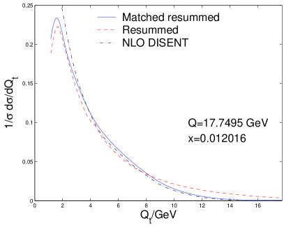
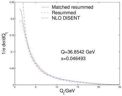
Figure 1: Comparison between DISENT [14], matched resummed and pure resummed differential distributions. MRST NLO pdfs have been used with $\alpha_{s}(M_{Z}^{2})=0.1205$ [25].

The aim of this section is to display the results obtained for a next-to–leading logarithmic resummed prediction matched to next-to–leading order predictions from DISENT [14]. Additionally we comment on the role that might be played by a non-perturbative Gaussian smearing function and that small-$x$ effects may effectively give an enhanced smearing of the spectrum leading to a broader prediction than the one provided here as was observed also in the SIDIS case [4, 6].

In Fig. 1, we display the fixed order NLO results along with the pure resummed and matched results for two values of the hard scale $Q$ and corresponding Bjorken $x$ values. The choice of the $x$ and $Q$ values correspond to bins where preliminary data already exist [13]. There one notes the divergent NLO result and the correct small $Q_{t}$ behaviour as given by the resummation as well as the role of matching in the high $Q_{t}$ tail of the distribution. We also point out that the role of the non-global term is limited to a few percent effect after the matching to fixed order has been performed. Thus missing uncalculated single-logarithmic terms in the non-global piece ${\mathcal{S}}$ that are suppressed as $1/N_{c}^{2}$, are not expected to change our quantitative conclusions.

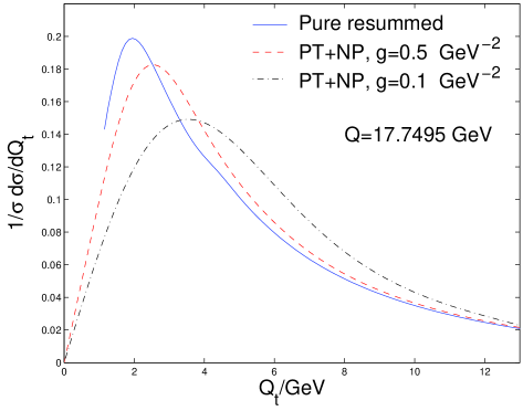
Figure 2: Non-perturbative smearing of the resummed prediction with a Gaussian function in $k_{t}$, $\exp[-gk_{t}^{2}]$. Two different choices of the smearing parameter $g$ are illustrated.

We also present here the effect of smearing or convoluting our resummation with a $b$ space or equivalent $k_{t}$ space Gaussian function representing non-perturbative effects. Such intrinsic $k_{t}$ effects have been the subject of much phenomenological investigation in Drell-Yan like processes [5, 22, 26, 27]. The non-perturbative smearing function we choose has the simple form $F^{\mathrm{NP}}(k_{t})=\exp[-gk_{t}^{2}]$ and we perform a two-dimensional convolution, $\int d^{2}{\vec{k}_{t}}\,g/\pi F^{\mathrm{NP}}\left(|\vec{Q_{t}}-\vec{k_{t}}|\right)I(k_{t})$ with the resummed distribution $I(k_{t})=1/\sigma\,d\sigma/dk_{t}^{2}$, to obtain the smeared result as a function of $Q_{t}$. We carry out the smearing with different values of $g$, two of which are illustrated in Fig. 2. The value of $g=0.5\,{\mathrm{GeV}}^{-2}$ corresponds to a reasonable mean intrinsic $k_{t}$ value of $1.25\,\mathrm{GeV}$. We also illustrate the effect of using a smaller $g$ value of $0.1\,{\mathrm{GeV}^{-2}}$, which leads as shown to a broader $Q_{t}$ distribution. Ideally one would need to compare our predictions with the data at different $x$ values in order to ascertain whether one sees any visible broadening of the NLL resummed spectra at smaller $x$, such as that mimicked by a change in the smearing parameter $g$. If this is the case one may investigate the dependence of the smearing parameter $g$ on Bjorken $x$, a step we leave to forthcoming work [15].

We should point out that in convoluting the resummed prediction with the non-perturbative Gaussian $k_{t}$ distribution it was necessary to provide an extrapolation of our resummed results for $I(k_{t})$ down to $k_{t}=0$. We have chosen this extrapolation as in Ref. [18] so as not to modify the NLL resummed result as well as to obtain the correct limiting behaviour of the integrated cross-section $\propto k_{t}^{2},$ as determined by evaluating the $b$ integral for the integrated quantity $\sigma(k_{t})$, in the limit $k_{t}\to 0$.

Thus we substitute for $k_{t}$ an effective variable $(k_{t}^{*})^{2}=k_{t}^{2}+Q_{0}^{2}\,\exp{\left(-k_{t}^{2}/Q_{0}^{2}\right)}$ and make the replacement $\sigma(k_{t})\to\sigma(k_{t}^{*})\left(1-\exp\left(-ak_{t}^{2}\right)\right)$, where $Q_{0}$ and $a$ should be chosen so as not to modify the resummed result in the range where it is valid, as in Ref. [18]. These additional parameters should only modify the very low (non-perturbative) $Q_{t}$ region where our NLL result is in any case not valid as it stands. One can think of the parameters $a$ and $Q_{0}$ as being non-perturbative inputs that can be varied alongside the smearing parameter $g$ to obtain a good fit to data in the lowest $Q_{t}$ region.

For the plot in Fig. 2 we chose to take $Q_{0}=1.2\,\mathrm{GeV}$ and $a=1/Q_{0}^{2}$ as these choices do not impact our resummed results over most of their range of validity. The dominant impact in the very low $Q_{t}$ region, beyond the control of NLL resummation, is in fact that of the smearing function $\exp{(-gk_{t}^{2})}$, for which different choices have been already mentioned.

6 Conclusions

We have introduced here a DIS variable that, as we have explained, has a very simple relationship to vector-boson and Higgs $Q_{t}$ spectra at hadron colliders. The aim of doing this has been to use HERA data to compare resummed theoretical predictions with experiment, keeping an eye on comparions at lower $x$ values. This complements the extensive studies of DIS event shapes that have been carried out thus far which employed the standard resummation formalism (and non-global logarithms), supplemented by $1/Q$ power corrections [10]. We recall that the program of comparing DIS event shapes to the data was quite successful without any special role visible for small-$x$ effects [9].

Given however that only moderately small $x$ values, $x\sim 10^{-2}$, can be reasonably accessed in these studies, it is clearly better to choose a variable that is potentially more sensitive to small-$x$ dynamics than event-shape variables, in order to determine the role of these effects. We expect such a variable to be the $Q_{t}$ spectrum we have defined here, where it will be interesting to establish if a small-$x$ enhanced broadening of the resummation we presented, is indeed visible in the data. This was apparently the case in SIDIS studies [6] and, if present, we expect these effects to manifest themselves for our observable too. Given the simple relationship of our results to those for Drell-Yan like observables it should then be easy to extrapolate our conclusions to hadron collider studies, where it is important to reach a firm conclusion on the issue of small-$x$ broadening.

At present we have preliminary data for our observable from HERA and we await the data in its final form before making detailed comparisons and drawing phenomenological conclusions on this issue. This will be the subject of forthcoming work.

Appendix A Leading order result

We report briefly below the leading-order result for $\sigma_{r}(Q_{t},Q)$, where $r$ denotes the resummed result, neglecting terms that vanish as $Q_{t}\to 0$. In line with the procedure of Ref. [7], the leading-order cross-section for events with $\left|\sum_{i\in{\mathcal{H}_{c}}}\vec{k}_{t,i}\right|<Q_{t}$ normalised to the Born cross-section is:

$$\sigma_{r}^{(1)}(Q_{t},Q,x)/\sigma_{0}=\frac{1}{q(x,Q^{2})}\frac{\alpha_{s}}{2\pi}\int_{x}^{1}\frac{d\xi}{\xi}\Bigg{\{}C_{F}\,q\left(\frac{x}{\xi},Q^{2}\right)\mathcal{F}_{q,2}\left(\xi,\frac{Q}{Q_{t}}\right)+\\ +T_{f}\,g\left(\frac{x}{\xi},Q^{2}\right)\mathcal{F}_{g,2}\left(\xi,\frac{Q}{Q_{t}}\right)-\frac{y^{2}}{1+(1-y)^{2}}\bigg{[}C_{F}\,q\left(\frac{x}{\xi},Q^{2}\right)\mathcal{F}_{q,L}\left(\xi,\frac{Q}{Q_{t}}\right)+\\ +T_{f}\,g\left(\frac{x}{\xi},Q^{2}\right)\mathcal{F}_{g,L}\left(\xi,\frac{Q}{Q_{t}}\right)\bigg{]}\Bigg{\}}\,,$$ (22)

where $y$ is the usual DIS Bjorken variable, $T_{f}=T_{R}\sum_{q\bar{q}}e_{q}^{2}$ and in the $\overline{\textrm{MS}}$ scheme we have:

$$\mathcal{F}_{q,2}\left(\xi,\frac{Q}{Q_{t}}\right)=\delta(1-\xi)\left[-2\ln^{2}\frac{Q}{Q_{t}}+3\ln\frac{Q}{Q_{t}}+\frac{3}{2}\ln 2-\frac{\pi^{2}}{2}-\frac{9}{2}\right]-2\left[\frac{1+\xi^{2}}{1-\xi}\right]_{+}\ln\frac{Q}{Q_{t}}+\\ +1-\xi-(1+\xi^{2})\Bigg{[}\frac{\theta(2\xi-1)}{1-\xi}\ln\frac{1-\xi}{\xi}\Bigg{]}_{+}-(12\xi^{3}-10\xi^{2}+1)\Bigg{[}\frac{\theta(2\xi-1)}{2(1-\xi)}\Bigg{]}_{+}\,,$$ (23)

$$\mathcal{F}_{g,2}\left(\xi,\frac{Q}{Q_{t}}\right)=-2[\xi^{2}+(1-\xi)^{2}]\ln\frac{Q}{Q_{t}}+2\xi(1-\xi)+\\ +\left\{(2\xi-1)(-6\xi^{2}+6\xi-1)-[\xi^{2}+(1-\xi)^{2}]\ln\frac{1-\xi}{\xi}\right\}\theta\left(2\xi-1\right),$$ (24)

$$\mathcal{F}_{q,L} = 2\xi\left(2\xi-1\right)\theta\left(2\xi-1\right),$$ (25)

$$\mathcal{F}_{g,L} = 4\xi(1-\xi)(2\xi-1)\theta\left(2\xi-1\right).$$ (26)

The $(2n_{f}+1)\times 1$ matrices $\textbf{\emph{C}}_{0}$ and $\textbf{\emph{C}}_{1}$ are defined such that their transposes are given by:

$$\textbf{\emph{C}}_{0}^{T}(z)=\left(\begin{array}[]{c}e_{u}^{2}\,\delta(1-z)\\ e_{u}^{2}\,\delta(1-z)\\ \vdots\\ 0\\ \end{array}\right),$$ (27)

and:

$$\textbf{\emph{C}}_{1}^{T}(z)=\left(\begin{array}[]{c}C_{F}\,e_{u}^{2}\left\{\mathcal{F}_{q,2}(z,1)-\frac{y^{2}}{1+(1-y)^{2}}\mathcal{F}_{q,L}(z,1)\right\}\\ C_{F}\,e_{u}^{2}\left\{\mathcal{F}_{q,2}(z,1)-\frac{y^{2}}{1+(1-y)^{2}}\mathcal{F}_{q,L}(z,1)\right\}\\ \vdots\\ T_{f}\left\{\mathcal{F}_{g,2}(z,1)-\frac{y^{2}}{1+(1-y)^{2}}\mathcal{F}_{g,L}(z,1)\right\}\\ \end{array}\right).$$ (28)

Appendix B The radiator

The radiator is given by:

$$R(Q/Q_{t})=Lg_{1}(\alpha_{s}L)+g_{2}(\alpha_{s}L)\,,$$ (29)

where $L=\ln(Q/Q_{t})$ and in the $\overline{\textrm{MS}}$ scheme:

$$g_{1}(\alpha_{s}L)=-\frac{C_{F}}{\pi\beta_{0}}\left[1+\frac{\ln(1-2\lambda)}{2\lambda}\right],$$ (30)

$$g_{2}(\alpha_{s}L)=\frac{3C_{F}}{4\pi\beta_{0}}\ln(1-2\lambda)+\frac{C_{F}K}{4\pi^{2}\beta_{0}^{2}}\left[\ln(1-2\lambda)+\frac{2\lambda}{1-2\lambda}\right]-\\ -\frac{C_{F}\beta_{1}}{2\pi\beta_{0}^{3}}\left[\frac{2\lambda+\ln(1-2\lambda)}{1-2\lambda}+\frac{1}{2}\ln^{2}(1-2\lambda)\right],$$ (31)

with $\lambda=\alpha_{s}(Q^{2})\beta_{0}L$ and:

$$K=C_{A}\left(\frac{67}{18}-\frac{\pi^{2}}{6}\right)-\frac{5}{9}n_{f}\,,\qquad\beta_{0}=\frac{11C_{A}-2n_{f}}{12\pi}\,,\qquad\beta_{1}=\frac{17C_{A}^{2}-5C_{A}n_{f}-3C_{F}n_{f}}{24\pi^{2}}\,.$$ (32)

In obtaining this, we used Eq.(13) and the 2-loop QCD $\beta$ function to replace the scale of $\alpha_{s}$ with $Q^{2}$ and moved from the CMW [17] scheme to the $\overline{\textrm{MS}}$ scheme (see e.g. Ref. [7]). The derivative of the radiator with respect to $\ln b$ at $\bar{b}\,Q=Q/Q_{t}$ is given by:

$$R^{\prime}(Q/Q_{t})=\frac{2C_{F}}{\pi\beta_{0}}\frac{\lambda}{1-2\lambda}\,.$$ (33)

The expansion of the resummed result (Eq.(19)) to $\mathcal{O}(\bar{\alpha}_{s})$ and $\mathcal{O}(\bar{\alpha}_{s}^{2})$, which is needed in Eq. (21), yields:

$$\sigma_{r}^{(1)}/\sigma_{0}=G_{11}L+G_{12}L^{2}-2\frac{\textbf{\emph{C}}_{0}\otimes\textbf{\emph{P}}\otimes\textbf{\emph{q}}(x,Q^{2})}{q(x,Q^{2})}L+\frac{\textbf{\emph{C}}_{1}\otimes\textbf{\emph{q}}(x,Q^{2})}{q(x,Q^{2})}\,,$$ (34)

$$\sigma_{r}^{(2)}/\sigma_{0}=G_{22}L^{2}+G_{23}L^{3}+\frac{1}{2}G_{12}^{2}L^{4}-2\left((G_{11}+2\pi\beta_{0})L^{2}+G_{12}L^{3}\right)\frac{\textbf{\emph{C}}_{0}\otimes\textbf{\emph{P}}\otimes\textbf{\emph{q}}(x,Q^{2})}{q(x,Q^{2})}\\ +\frac{\textbf{\emph{C}}_{1}\otimes\textbf{\emph{q}}(x,Q^{2})}{q(x,Q^{2})}\left(G_{11}L+G_{12}L^{2}\right)+2\frac{\textbf{\emph{C}}_{0}\otimes\textbf{\emph{P}}\otimes\textbf{\emph{P}}\otimes\textbf{\emph{q}}(x,Q^{2})}{q(x,Q^{2})}L^{2}\,,$$ (35)

where P is the matrix of leading order splitting functions and the coefficients $G_{mn}$ are given in table 1. One can clearly see that the expansion of the resummed result to $\mathcal{O}(\alpha_{s})$ reproduces the leading order result given by Eq. (22).

$\,G_{12}\,$	$\,-2\,C_{F}$
$\,G_{11}\,$	$\,3\,C_{F}$
$\,G_{23}\,$	$\,-6\,C_{F}^{2}-\frac{16}{3}\pi\,C_{F}\beta_{0}$
$\,G_{22}\,$	$\,-\frac{\pi^{2}}{3}C_{F}C_{A}+\frac{9}{2}\,C_{F}^{2}-2\,C_{F}K+6\,\pi\,C_{F}\beta_{0}$

Table 1: The coefficient $G_{nm}$ that enter the fixed-order expansion of the resummed result.

References

- [1] See e.g. proceedings of the HERA-LHC workshop [hep-ph/0601013, hep-ph/0601012].
- [2] G. Bozzi, S. Catani, D. de Florian and M. Grazzini, Nucl. Phys. B 737 (2006) 73 [hep-ph/0508068].
- [3] D. de Florian, M. Grazzini and Z. Kunszt, Phys. Rev. Lett. 82 (1999) 5209 [hep-ph/9902483].
- [4] S. Berge, P. M. Nadolsky, F. I. Olness and C.-P. Yuan, Phys. Rev. D 72 (2005) 033015 [hep-ph/0410375].
- [5] J. C. Collins, D. E. Soper and G. Sterman, Nucl. Phys. B 250 (1985) 199.
- [6] P. Nadolsky, D. R. Stump and C.-P. Yuan, Phys. Rev. D 61 (2000) 014003, Erratum-ibid. D 64 (2001) 059903 [hep-ph/9906280].
- [7] M. Dasgupta and G. P. Salam, Eur. Phys. J. C 24 (2002) 213 [hep-ph/0110213].
- [8] V. Antonelli, M. Dasgupta, G. P. Salam, J. High Energy Phys. 0002 (2000) 001 [hep-ph/9912488].
- [9] M. Dasgupta and G. P. Salam, J. High Energy Phys. 0208 (2002) 032 [hep-ph/0208073].
- [10] M. Dasgupta and B. R. Webber, Eur. Phys. J. C 1 (1998) 539 [hep-ph/9704297].
- [11] M. Dasgupta and G. P. Salam, Phys. Lett. B 512 (2001) 323 [hep-ph/0104277].
- [12] M. Dasgupta and G. P. Salam, J. High Energy Phys. 0203 (2002) 17 [hep-ph/0203009].
- [13] T. Kluge, private communication.
-
[14]
S. Catani and M. H. Seymour, Phys. Lett. B 378 (1996) 287 [hep-ph/9602277],
S. Catani and M. H. Seymour, Nucl. Phys. B 485 (1997) 291 [hep-ph/9605323]. - [15] M. Dasgupta and Y. Delenda, work in progress.
- [16] G. Parisi and R. Petronzio, Nucl. Phys. B 154 (1979) 427.
- [17] S. Catani, B. R. Webber and G. Marchesini, Nucl. Phys. B 349 (1991) 635.
- [18] R. K. Ellis and S. Veseli, Nucl. Phys. B 511 (1998) 649 [hep-ph/9706526].
- [19] S. Frixione, P. Nason and G. Ridolfi, Nucl. Phys. B 542 (1999) 311 [hep-ph/9809367].
- [20] J. W. Qiu and X. f. Zhang, Phys. Rev. Lett. 86 (2001) 2724 [hep-ph/0012058], Phys. Rev. D 63 (2001) 114011 [hep-ph/0012348].
- [21] C. T. H. Davies, B. R. Webber and W. J. Stirling, Nucl. Phys. B 256 (1985) 413.
- [22] G. Ladinsky and C.-P. Yuan, Phys. Rev. D 50 (1994) 4239 [hep-ph/9311341].
- [23] F. Landry, R. Brock, P. M. Nadolsky and C.-P. Yuan, Phys. Rev. D 67 (2003) 073016 [hep-ph/0212159].
- [24] A. V. Konychev and P. M. Nadolsky, Phys. Lett. B 633 (2006) 710 [hep-ph/0506225].
- [25] A. D. Martin, R. G. Roberts,W. J. Stirling and R. S. Thorne, Phys. Lett. B 604 (2004) 61 [hep-ph/0410230].
- [26] S. Tafat, J. High Energy Phys. 0105 (2001) 004 [hep-ph/0102237].
- [27] F. Landry, R. Brock, G. Ladinsky and C.-P. Yuan,Phys. Rev. D 63 (2001) 013004 [hep-ph/9905391].