OPEN PROBLEMS IN HYDRODYNAMICAL APPROACH
TO RELATIVISTIC HEAVY ION COLLISIONS

Abstract

We discuss some open problems in hydrodynamical approach to the relativistic heavy ion collisions. In particular, we propose a new, very simple alternative approach to the relativistic dissipative hydrodynamics of Israel and Stewart.

1 Introduction

The phase transitions in strongly interacting bulk matter predicted by the quantum chromodynamics (QCD) should manifest their existence in different physical scenarios such as the evolution of inhomogeneities in the early universe, structure of compact stars, spectra of particles from nuclear collisions at ultra-relativistic energies, etc. In particular, the relativistic heavy ion collisions are the unique possibility of observing such phase transitions in laboratories, permitting us to extract the bulk properties of the strongly interacting matter at extremely high temperature and energy density.

As we see from many talks in this conference, the over-all “picture” of the new states of the matter at extreme condition achieved in the laboratories (mainly from SPS and RHIC) is now being configured after more than two decades when the first project on relativistic heavy ion physics started[1]. Yet the nature of the transition from the hadronic phase to the QGP phase is still to be clarified quantitatively. Of course, in addition to the experimental data, advances in theoretical studies such as lattice QCD calculations also enriched understandings of the properties of the strong interacting matter[2, 3].

Among many signals of QGP, the one which brought a new insight is the emergence of collective flow in the final state of exploding particles. In the non-central collisions, an asymmetric distribution of energy density is created in the first instant of the collision. In the hydrodynamical image, the driving force to expand the system is proportional to the pressure gradient, so that this asymmetry with respect to the direction of the largest pressure gradient should increase as a function of the transverse momenta of particles. Quantitatively, such anisotropy can be expressed in terms of the coefficients of Fourier series of the azimuthal distribution of particles. We define the elliptic flow for a given transverse momentum window as

$$v^{\left(2\right)}\left(p_{T}\right)=\frac{\left\langle\int d\phi\ \left[d^{2}N/dp_{{}_{T}}^{2}d\phi\right]\cos 2\left(\phi-\phi_{\vec{b}}\right)\right\rangle}{\left\langle\int d\phi\ \left[d^{2}N/dp_{{}_{T}}^{2}d\phi\right]\right\rangle},$$

where $p_{{}_{T}}$ is the transverse momentum, and $\phi$ and $\phi_{\vec{b}}$ are, respectively, the azimuthal angles of the particle and of the impact parameter vector with respect to a some space-fixed coordinate system. In practice, the determination of these coefficients from the experimental data is not trivial since the reaction plane is not given a priori. In the hydrodynamical calculations, of course the reaction plane is given from the beginning.

The finite positive value of this coefficient $v_{2}$ is referred to as the elliptic flow and, from the point of view of hydrodynamics, it is sensitive to the initial pressure gradient of the system. The above expected behavior of $v_{2}$ was clearly observed in RHIC data, and the values of observed values approach to those calculated from the ideal hydrodynamics. At the same time, for lower (SPS) energies, the experimental values are lower than the ideal fluid values (See Figs.1 and 2). This fact was interpreted as the emergence of the new state of the matter which flows almost as an ideal fluid, while in the hadronic phase the matter suffers from the collisional viscosity[4].

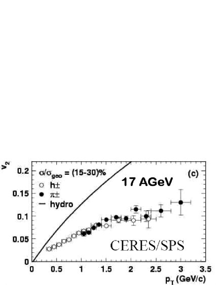
Figure 1: Elliptic flow at SPS energies as function of transverse momentum, compared to the simple ideal fluid hydrodynamical calculation. The observed values of elliptic flow are below the hydro values. Figure adapted from the presentation of M. Gyulassy, see this volume

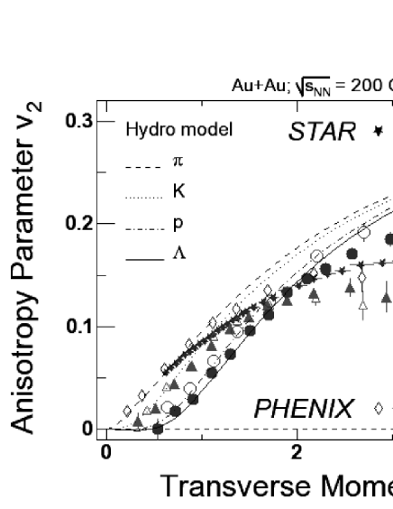
Figure 2: Elliptic flow at RHIC energies as function of transverse momentum, compared to the simple ideal fluid hydrodynamical calculation. Figure adapted from the presentation of M. Gyulassy, see this volume

In addition to the behavior of the elliptic flow phenomena, hydrodynamical description is found to be very successful in many aspects of SPS and RHIC data[5], thus establishing the general physical scenario of strongly interacting matter in the process of relativistic heavy ion collisions. On the other hand, this remarkable success of the hydrodynamics opens several important questions and understanding of these questions may lead us to some new physical concepts. In this paper, we discuss some of these questions.

2 Relativistic Hydrodynamics

The hydrodynamical description in nuclear and particle physics is not new[7]. However, it is also true that to establish a solid theoretical foundation for the application of hydrodynamical description to microscopic systems has always been difficult. This is basically because the starting assumption of the validity of local thermodynamical equilibrium in hydrodynamics is not at all trivial to be justified for microscopic systems.

For the sake of later discussion, let us here summarize briefly the basic structure of the relativistic hydrodynamics[8]. Let $T^{\mu\nu}$ be the energy-momentum tensor of the matter. Then the dynamics of the system should obey the conservation law of this tensor,

$$\partial_{\mu}T^{\mu\nu}=0.$$ (1)

For the case of a perfect fluid in local equilibrium, we can write

$$T^{\mu\nu}=\left(\varepsilon+p\right)u^{\mu}u^{\nu}-pg^{\mu\nu},$$ (2)

where $\varepsilon,p$ and $u^{\mu}$ are, respectively, the proper energy density, pressure and four-velocity of the fluid element. Eq.(1) should be complemented by the continuity equations for conserved currents such as the baryon number,

$$\partial^{\mu}\left(nu_{\mu}\right)=0,$$ (3)

and also the equation of state which describes the thermodynamical properties of the matter. The equation of state may be specified in the form of

$$\varepsilon=\varepsilon\left(n,s\right),$$ (4)

where $n$ and $s$ are the baryon number and the entropy densities, respectively. For ideal fluid case, we can also derive the conservation of entropy,

$$\partial^{\mu}\left(su_{\mu}\right)=0.$$ (5)

from Eqs.(1,2) and (3) using the Gibbs-Duhem relation,

$$dp=\mu dn+Tds,$$ (6)

which can be uniquely determined once Eq.(4) is specified, together with the first law of thermodynamics, $d\varepsilon=Tds+\mu dn$ and the Euler relation for extensivity $\varepsilon+p=Ts+\mu n.$

These hydrodynamical equations can also be derived from the action principle[9]. They can be solved numerically to give the space-time development of all the necessary thermodynamical variables and the fluid velocity[10, 5].

3 Some Open Problems of Relativistic Hydrodynamics

As mentioned in Introduction, the ideal hydrodynamical description for the dynamics of hot and dense matter observed in RHIC experiments works amazingly well, especially for the collective flow. The success of the approach indicates that the very early equilibration of the partonic gas takes place. The nature of the QGP seems rather a strongly interacting fluid (sQGP) than a ideal free parton gas[6]. On the other hand, there exist several open problems in the interpretation of data in terms of the hydro model. These questions require careful examination to extract quantitative and precise information on the properties of QGP. Furthermore, one should note that several very different physical scenarios within the hydrodynamical approach (e.g. the use of continuous emission, sudden freeze-out and rQMD final state cascade, or some drastically simplified hydro models such as blast wave solution, etc.) can give rise equally good results in reproducing the observables with suitable choices of parameters. In a way, one may say that the hydro signature is “robust”, but on the other hand, this could be a synonym of “insensitive”. In order to extract more precise information on the properties of the quark-gluon plasma and the mechanism of phase transition in the bulk QCD matter, we should clarify these points and refine the physical parameters used in these approaches.

With respect to this point, one should remind a important point of the collective flow. When we use the equation of state to describe the pressure as function of density, the hydrodynamical equations are meaningful only if the approximation of local thermal equilibrium is valid. On the other hand, as far as Eq.(1) is concerned, it is nothing but the local conservation of energy and momentum density. Therefore, it may be possible that a system which is completely out of local thermal equilibrium can also manifest a flow pattern depending on the origin of the force. For example, as a well-known example, we may recall that the Schrödinger equation

$$i\hbar\frac{\partial\psi}{\partial t}=-\frac{\hbar^{2}}{2m}\nabla^{2}\psi+V\psi$$

can also be written just as if the form of hydrodynamics,

$$\frac{\partial}{\partial t}\vec{v}+\left(\vec{v}\cdot\nabla\right)\vec{v} =-\frac{1}{m}\nabla p_{q}-\frac{1}{m}\nabla V,$$

$$\frac{\partial n}{\partial t}+\nabla\cdot\left(n\vec{v}\right) =0,$$

where

$$\vec{v}=\frac{1}{m}\nabla\left(\arg\psi\right),\ \ \ \ n=\left|\psi\right|^{2}.$$

Here,

$$p_{q}=-\frac{1}{2m}\frac{1}{\left|\psi\right|}\nabla^{2}\left|\psi\right|$$

comes from the quantum uncertainty principle and serves as the pressure, but nothing to do with the thermal equilibrium. In this example, the “pressure gradient”comes from the quantum uncertainty principle. That is, a flow phenomena does not necessarily indicates the validity of the local thermodynamical equilibrium.

In the following, we list several crucial points of the hydrodynamical approach to the relativistic heavy ion reactions.

• Initial conditions

When two nuclei collide, a huge number of partonic degrees of freedom are excited. At the first instant of the collision, these partonic degrees of freedom are far from thermal equilibrium. To obtain the initial condition suitable for the hydrodynamical scenario, we should understand how these partonic degrees of freedom reach the local equilibrium state, forming the quark-gluon plasma. It seems that the time scale to achieve the thermal equilibrium in partonic cascade calculation within reasonable values of parton cross section is much larger than the time scale required for the hydrodynamical models. Thus the success of hydrodynamics cast a very interesting question of how such an early thermalization can be attained in the initially created QCD partonic excitations. Several new concepts have been proposed. For example, as the mechanism of quick isotropization from the initial momentum distribution of partons (which is predominantly longitudinal), the so-called Weibel instabilities known in plasma physics is shown to be effective also in the case of QCD[11, 12, 13].

However, the isotropization itself is a necessary but not a sufficient condition for the thermal equilibrium. With respect to the mechanism of thermalization, another interesting notion, called pre-thermalization, is recently developed. In a scalar field theoretical model, it is shown that when the system is set to an excited state, the validity of equation of state (the functional relation between energy density and pressure) is attained well before the real thermal equilibrium is reached[25]. With respect to this point, we have discussed a possible relation between the mechanism of early thermalization to the non-extended statistical mechanics[26]. Furthermore, the approach from the color glass condensate may provide an initial momentum distribution easy to achieve a quick thermalized state of partons because of saturation mechanism. Several investigations based on the CGC approach to calculate the initial energy distribution have been carried out[15].

• Event-by-event fluctuations.

Even the mechanism of thermalization is fast enough, the initial condition attained by high energy nuclear collision event is far from smooth as shown by the event generators such as NeXUS code[14]. Furthermore, this initial configuration fluctuates collision by collision very largely, even for central collision of heavy nuclei. It has been pointed out that the effect of even-by-event fluctuations due to the different initial conditions are crucial for quantitative studies of observables such as elliptic flow[16]. Since the dynamical evolution of hydrodynamics is extremely nonlinear, the event average of any hydrodynamical obserbable is quite different from the value calculated from the averaged smooth initial configuration, which is the hydrodynamcal calculations commonly used. The fluctuation of $v_{2}$ coefficient must contain the dynamical information of the state formed in the early stage of the collision.

• Finite size effect

Strictly speaking, the hydrodynamics is essentially the zero mean-free path (or correlation length) approximation for the microscopic degrees of freedom compared to the system size. For the nuclear collisions, this is not a trivial approximation. As we know that the nuclear ground state has finite surface thickness (of the order of 3 fm) but if we try to describe the density distribution in terms of zero mean free-path hydrodynamics, we would have zero surface thickness for the ground state mass distribution. The parameter which characterizes the degree of approximation with respect to the finite size of the system would be

$$x=\frac{\lambda_{micro}}{\lambda_{Hydro}}$$

where $\lambda_{micro}$ is the typical mean-free path (or the correlation length) of the constituent particles and $\lambda_{Hydro}$ is the hydrodynamical inhomogeneity scale, which is typically

$$\lambda_{Hydro}\simeq\left|\frac{1}{\rho}\nabla\rho\right|^{-1}.$$ (7)

Hydrodynamics is valid for $x\ll 1$, so that when the local inhomogeneity scale in the system is of the order of the mean-free path, the hydrodynamics should break down.

In order to take into account for the finite $x$ values, as relativistic extension of the Weizsäcker term, we may introduce the gradient term in the action of hydrodynamics as

$$I=\int d^{4}x\ \left[-\varepsilon\left(n,s\right)+\frac{1}{2}\sigma\left(\nabla^{\mu}n\right)^{2}\right],$$

where $\sigma$ is a quantity related to the surface tension in the static limit and $\nabla^{\mu}$ is the four-gradient projected to the hyperplane perpendicular to the velocity,

$$\nabla^{\mu}=\left(g^{\mu\nu}-u^{\mu}u^{\nu}\right)\partial_{\nu}=P^{\mu\nu}\partial_{\nu}.$$

where $P^{\mu\nu}=$ $\left(g^{\mu\nu}-u^{\mu}u^{\nu}\right)$ is the projection operator to the hypersurface perpendicular to the four-velocity $u^{\mu}$. The general energy-momentum conservation can be obtained from the Nöther theorem and the resulting equation of motion (for constant $\sigma$ case) becomes

$$\partial_{\mu}\widetilde{T}^{\mu\nu}=-\partial_{\mu}\left(\sigma(\nabla^{\mu}n)(\partial^{\nu}n)-\sigma\dot{n}u^{\mu}\nabla^{\nu}n-\frac{\sigma}{2}g^{\mu\nu}(\nabla^{\tau}n)(\partial_{\tau}n)\right)$$

where

$$\widetilde{T}^{\mu\nu}=\varepsilon u^{\mu}u^{\nu}-P^{\mu\nu}\widetilde{p}$$

with

$$\widetilde{p}=p+\sigma n\partial_{\nu}(\nabla^{\nu}n).$$

Unfortunately, the above equation becomes dynamically much more complicated than the usual hydrodynamics. In any case, the finite size effect on the local energy density is an important question, in particular with respect to the properties of phase transition. A further investigation on this direction is now in progress[18].

• Viscosity effects.

The comparison of flow phenomena to the ideal fluid calculation indicates that the emergence of new state of matter which flows like an ideal-fluid at RHIC energies. This idea that the QGP behaves a real ideal fluid raised an interesting question when the viscosity for the strong coupling limit of 4D conformal theory obtained from the supersymmetric string theory found to be a very small[19]. On the other hand, Hirano and Gyulassy argue that this is due to the entropy density of the QGP which is much larger than the hadronic phase[4]. To be precise, a quantitative and consistent analysis of the viscosity within the framework of relativistic hydrodynamics has not yet been done completely. This is because the introduction of dissipative phenomena in relativistic hydrodynamics casts difficult problems, both conceptual and technical. Several works have been done in this direction[32]. We will discuss later this point more in detail in the next section.

• Final hadron spectra from the hydrodynamical model.

To analyze the physical observables in terms of the hydrodynamical scenario, we have to construct the particle spectra from the hydro solution. As the hydrodynamical expansion proceeds, the fluid becomes cooled down and rarefied, thus leading to the decoupling of the constituent particles. At this stage, these particles do not interact any more and free-stream to the detector. Long-lived resonances and other unstable particles may decay on the way to the detector after this instant of decoupling phase. In the standard hydrodynamical models, one introduces the concept of freeze-out, which assumes that particle emission occurs on a sharp three-dimensional surface (defined for example by the local temperature, $T(x,y,z,t)=$ constant). Before crossing it, particles have a hydrodynamical behavior, and after they free-stream toward the detectors, keeping memory of the conditions (flow, temperature) of where and when they crossed the three dimensional surface. The Cooper-Frye formula [20] gives the invariant momentum distribution in this case

$$Ed^{3}N/dp^{3}=\int_{\sigma}d\sigma_{\mu}p^{\mu}f(x,p).$$ (8)

$d\sigma_{\mu}$ is the surface element 4-vector of the freeze out surface $\sigma$ and $f$ the thermal distribution function of the type of particles considered. The space-time dependence comes from those of thermodynamical parameters, such as temperature and chemical potential. This is the formula implicitly used in all standard thermal and hydrodynamical model calculations.

Although simple and elegant, this sudden freeze-out is not only an idealization but also contains some problems such as conservation of energy and momentum, negative flux and artificial entropy production[8]. To remedy this approach several approaches have been proposed such as the use of URQMD code coupled to the final state of the hydrodynamics[22, 23]. However, usually these calculations are rather complex and time consuming in practice.

The most important effect which should effect the form of particle spectra is that not every particles are emitted from the same hypersurface specified by a unique temperature. The continuous emission approach[21] still uses the equilibrium momentum distribution of particles but they can be emitted continuously during the hydrodynamical evolution of the system. It also takes into account the absorption effects while the emitted particle from the inside traverses the surrounding hadronic matter. This accounts for the finite size of the system in the final particle spectra. In contrast to the usual sudden freeze-out, it is found that the final hadrons can be emitted from a broad range of temperatures. It should be emphasized that the two extremely cases, a sharp temperature surface of sudden freeze-out and almost flat distribution of temperature of the continuous emission scenario give equally good description of the observed spectra and flow[5].

4 Viscosity and Causality

To extract more precise quantitative conclusion on the ideal nature of the QGP fluid, we should study the effect of dissipative processes on the collective flow variables. However, a covariant theory of dissipative phenomena is not trivial at all. We know that the diffusion equation is not covariant, and the equation is parabolic so that the propagation of signal has an infinite velocity. Landau introduced the dissipative effects in the relativistic hydrodynamics, but it is known that the formalism of Landau[7] of relativistic viscous fluid still leads to the problem of acausalily. Relativistic covariance is not the sufficient condition for a consistent relativistic dissipative dynamics. To cure this problem, the second order thermodynamics was developed by Israel, Stewart and Miller[31]. However, this theory is too general and complex, containing many unknown parameters which make difficult the application of the theory to practical problems. Furthermore, the theory contains the third order time derivatives, introducing additional difficulties of initial value problem and numerical procedure. In our opinion, this is not the unique approach to the consistent relativistic dissipative hydrodynamics. Here, we show that an alternative theory which satisfies the minimum conditions of covariance and causal propagation of signal, and in the small viscosity limit, it recovers the usual ideal hydrodynamics.

To this, we first note that the problem of acausal propagation in usual diffusion equation,

$$\frac{\partial}{\partial t}n=-\zeta\nabla^{2}n$$

can be cured by the introduction of the relaxation time as

$$\tau_{relax}\frac{\partial^{2}n}{\partial t^{2}}+\frac{\partial n}{\partial t}=\zeta\nabla^{2}n,$$ (9)

converting the parabolic equation to the hyperbolic equation. For a suitable choice of parameters, $\tau_{relax}$, we can recover the causal propagation of the diffusion fluxLABEL:MorseFeshbach. Physically this can be understood as following. In general, the diffusion equation is the combination of two equations,

• Continuity equation,

  $$\frac{\partial n}{\partial t}+\nabla\cdot\vec{j}=0,$$ (10)

• Generation of the irreversible current due to the thermodynamical force,

  $$\vec{j}=-L\nabla\frac{\delta F\left(n\right)}{\delta n}$$ (11)

  and within the linear response of the system, we have

  $$\vec{j}=-\zeta\nabla n$$

  where $F$ is the thermodynamical potential and $\zeta$ is in general a function of thermodynamical quantities, but here we assume to be constant for the sake of simplicity.

The origin of acausality resides in Eq.(11) than the continuity equation, (10), since this means that the action of the force $\nabla\left(\delta F/\delta n\right)$ immediately generates the physical current $\vec{j}.$ We may think of relaxation phenomena for this process. This can be done phenomenologically by introducing the retardation function

$$G\left(t,t^{\prime}\right)=\frac{1}{\tau_{relax}}e^{-\left(t-t^{\prime}\right)/\tau_{relax}}$$ (12)

and rewrite Eq.(11) as

$$\vec{j}=-\int_{-\infty}^{t}G\left(t,t^{\prime}\right)\nabla F\left(\vec{r},t^{\prime}\right)dt^{\prime}.$$

In the limit of $\tau_{relax}\rightarrow 0,$ we have $G\left(t,t^{\prime}\right)\rightarrow\delta\left(t-t^{\prime}\right)$ so that this recovers the original equation, (11). Now

$$\frac{\partial\vec{j}}{\partial t}=-\frac{1}{\tau_{relax}}\nabla F-\frac{1}{\tau_{relax}}\vec{j}.$$

Taking the time derivative of Eq.(10) and substituting the above equation,

$$\frac{\partial^{2}n}{\partial t^{2}} = \nabla\cdot\left(\frac{1}{\tau_{relax}}\nabla F+\frac{1}{\tau_{relax}}\vec{j}\right)$$

$$= \frac{1}{\tau_{relax}}\left(-\frac{\partial n}{\partial t}+\nabla^{2}F\right)$$

obtaining Eq.(9). Eq.(9) is usually referred to as telegraphic equation. For more microscopic derivation of telegraphic equation, see [28, 29, 30].

We use the above mechanism to derive the relativistic dissipative hydrodynamics to transform the Landau formulation to satisfy causality. For this purpose, first let us review briefly the essential part of the Landau derivation of the relativistic dissipative hydrodynamics. Landau requires the conservation laws,

$$\partial_{\mu}T^{\mu\nu} = 0,$$ (13)

$$\partial_{\mu}N^{\mu} = 0.$$ (14)

In the presence of dissipative phenomena, the energy momentum tensor $T^{\mu\nu}$ and the baryonic current $N^{\mu}$ are not given by Eqs.(2) (3) anymore, but instead,

$$T^{\mu\nu}=\varepsilon u^{\mu}u^{\nu}-P^{\mu\nu}\left(p+\Pi\right)+\pi^{\mu\nu},$$ (15)

$$N^{\mu}=nu^{\mu}+\nu^{\mu},$$ (16)

where $\Pi$ and $\pi^{\mu\nu}$ are the bulk and shear viscous stresses, respectively and $\nu^{\mu}$ is the diffusion current of baryon number. For these, we require the constraints, $u_{\mu}\pi^{\mu\nu}=0$ and $u_{\mu}\nu^{\mu}=0.$ With these terms, of course the conservation of entropy Eq.(5) is not valid anymore, instead we have

$$\partial_{\mu}\left(su^{\mu}-\alpha\nu^{\mu}\right)=\frac{1}{T}\left(-P^{\mu\nu}\Pi+\pi^{\mu\nu}\right)\partial_{\mu}u_{\nu}-\nu^{\mu}\partial_{\mu}\alpha,$$ (17)

where $\alpha=\mu/T$. Landau identifies the term

$$\sigma^{\mu}=su^{\mu}-\alpha\nu^{\mu}$$ (18)

as the entropy current and requires the positive definiteness of the right-hand side of Eq.(17) as

$$\frac{1}{T}\left(-P^{\mu\nu}\Pi+\pi^{\mu\nu}\right)\partial_{\mu}u_{\nu}-\nu^{\mu}\partial_{\mu}\alpha\geq 0,$$ (19)

obtaining the following expressions for the viscous terms,

$$\Pi=\zeta\partial_{\alpha}u^{\alpha},\ \ \ \widetilde{\pi}_{\mu\nu}=\eta\partial_{\mu}u_{\nu},\ \ \ \widetilde{\nu}_{\mu}=-\kappa\partial_{\mu}\alpha$$ (20)

and introduce the projection operator to satisfy the orthogonality condition for the viscous term to the fluid velocity as

$$\pi^{\mu\nu}=P^{\mu\alpha\nu\beta}\widetilde{\pi}_{\alpha\beta},\ \ \nu^{\mu}=P^{\mu\alpha}\widetilde{\nu}_{\mu},$$ (21)

where $P^{\mu\alpha\nu\beta}$ is the double symmetric traceless projection,

$$P^{\mu\alpha\nu\beta}=\frac{1}{2}\left(P^{\mu\alpha}P^{\nu\beta}+P^{\nu\alpha}P^{\nu\nu}\right)-\frac{1}{3}P^{\mu\nu}P^{\alpha\beta}.$$ (22)

As mentioned, this Landau scheme leads to the acausal propagation of thermal current. However, at this moment, generalization of these equation in order to obtain to hyperbolic equations is self-evident. We introduce the retardation integral in each viscous term before the projection,

$$\Pi = -\int^{\tau}d\tau^{\prime}G\left(\tau,\tau^{\prime}\right)\zeta\partial_{\alpha}u^{\alpha}\left(\tau^{\prime}\right),$$ (23)

$$\tilde{\pi}^{\mu\nu} = \int^{\tau}d\tau^{\prime}G\left(\tau,\tau^{\prime}\right)\partial^{\mu}u^{\nu}\left(\tau^{\prime}\right),$$ (24)

$$\widetilde{\nu}^{\mu} = -\int^{\tau}d\tau^{\prime}G\left(\tau,\tau^{\prime}\right)\kappa\partial^{\mu}\alpha\left(\tau^{\prime}\right),$$ (25)

where $\tau$ is the local proper time. These integrals are equivalent to the differential equations

$$\Pi = -\zeta\partial_{\alpha}u^{\alpha}+\gamma\frac{d\Pi}{d\tau}$$ (26)

$$\tilde{\pi}^{\mu\nu} = \eta\partial^{\mu}u^{\nu}-\gamma\frac{d\tilde{\pi}^{\mu\nu}}{d\tau}$$ (27)

$$\widetilde{\nu}^{\mu} = -\kappa\partial^{\mu}\alpha+\gamma\frac{d\widetilde{\nu}^{\mu}}{d\tau}$$ (28)

with

$$\frac{d}{d\tau}=u^{\mu}\partial_{\mu}$$

is the total derivative with respect to the proper time. These equations, after the projection (Eq.21), can be compared to the Israel-Stewart form,

$$\Pi = -\zeta\left(\partial_{\alpha}u^{\alpha}-\beta_{{}_{0}}\frac{d\Pi}{d\tau}-\alpha_{{}_{0}}\partial_{\alpha}\nu^{\alpha}\right)$$ (29)

$$\pi^{\mu\nu} = \eta P^{\mu\alpha\nu\beta}\left(\partial_{\alpha}u_{\beta}-\beta_{2}\frac{d\pi^{\mu\nu}}{d\tau}-\alpha_{{}_{1}}\partial_{\alpha}\nu_{\beta}\right)$$ (30)

$$\nu^{\mu} = -\kappa p^{\mu\nu}\left(\partial_{\nu}\alpha-\beta_{1}\frac{d\nu^{\nu}}{d\tau}+\alpha_{{}_{0}}\partial_{\nu}\Pi+\alpha_{{}_{1}}\partial_{\alpha}\pi_{\nu}^{\alpha}\right).$$ (31)

They are similar, but we can see that the Israel-Stewart form contains the more general linear combination of the second order variables. However, the most important and essential difference is that, in our formalism, the projection operators $P^{\mu\nu}$ enter after the integration of these equations. All the dissipative terms are expressed explicitly in terms of independent variables of the usual hydrodynamics. In the Israel-Stewart form, due to the projection operators, integral form as Eqs.(23,24,25) can not be obtained explicitly.

Our approach has several advantages to the Israel-Stewart formalism. First of all, we keep the simple physical structure of Landau formalism, but at the same time we cured its causality problem by introduction of the relaxation integral, Eqs.(23,24,25). Use of these integral expressions also eliminates the problem of higher derivatives in time. We only need the past values of the independent variables to solve numerically. This also eliminates the problem of extra initial conditions, too. The integral expressions are easy to be evaluated when we use the Lagrangian coordinate system such as SPHERIO[10, 5]. Because of the simple form of viscous terms, incorporation of these equations to the realistic hydro-code such as SPHERIO is relatively easy. A work on this line is in progress.

5 Summary

The hydrodynamics is found to be a very successful tool for the description of the relativistic heavy ion collisions. However, from the quantitative point of view, the present hydrodynamical approach still contains many uncertainties and also some conceptual problems. In this paper, we call attention to these questions, and discussed some of problems in detail. In particular, we propose an alternative theory to the Israel-Stewart second order thermodynamics, where viscous terms are given by the integral expressions which take into account of the relaxation time. In this way, the problem of causality is avoided and at the same time a simple physical structure of Landau formulation has been kept. Other questions as early thermalization, finite size effects, fluctuations in initial conditions, etc. should also be studied more in detail When these questions are clarified, we will have much more detailed knowledge about the dynamics and properties of the new states of strongly interacting matter. It is also quite important to look for signals of genuine hydrodynamics, such as shock wave propagation[33].

This work is dedicated to Prof. W. Greiner, one of the pioneers of the subject, on the occasion of his 70th birthday. The authors express their thanks to H. M. Kiriyama, F. Grassi, Y. Hama, C.E. Aguiar and E. Fraga for stimulating discussions and kind help. T.Kodama is also grateful for the kind hospitality of Prof. H. Stöcker during his stay in Frankfurt. This work was partially supported by FAPERJ, FAPESP, CNPQ and CAPES.

References

- [1] For example talks of J. Harris, L. Csernai, M. Gyulassy, J. Rafelski, J. Stachel, L.McLerran, N.Xu, G. Ritter and S. Baas in this volume.
- [2] F. Karsch, Nucl. Phys. A 698, 199 (2002).
- [3] Z. Fodor and S. D. Katz, Phys. Lett. B 534, 87 (2002).
- [4] T. Hirano and M. Gyulassi, nucl-th/0506049, see also M. Gyulassy, this volume.
- [5] Y. Hama, T. Kodama and O. Socolowski, Braz.J.Phys.35, 24-51 (2005).
- [6] E. Shuryak, Prog. Part. Nucl. Phys. 53, 273 (2004).
- [7] L.D. Landau, Izv. Akad. Nauk SSSR Ser. Fiz. 17, 51 (1953), W. Greiner, W. Scheid and H. Muller) Phys. Rev. Lett. 32, 741 (1974)
- [8] L.P. Csernai: Introduction to Relativistic Heavy Ion Collisions, Wiley, New York, 1994. See also R.B. Clare and D. Strottman, Phys. Rep. 141, 177 (1986), H. Stöcker and W. Greiner, Phys. Rep. 137, 277 (1986).
- [9] H. T. Elze, Y. Hama, T. Kodama, M. Makler and J. Rafelski, J. Phys. G25, 1935 (1999).
- [10] C.E.Aguiar, T.Kodama, T.Osada and Y.Hama, J. Phys. G27, 75 (2001).
- [11] J. Randrup and S. Mrowczynski, Phys.Rev.C68:034909, 2003
- [12] P. Romatschke and M. Strickland, Phys.Rev.D70, 116006 (2004), A. Dumitru, Y. Nara and M. Strickland, hep-ph/0604149
- [13] P. Arnold and J. Lenaghan, Phys.Rev. D70 114007 (2004).
- [14] X.N. Wang and M. Gyulassy, Phys.Rev. D44, 3501 (1991), K.Geiger and D.Srivastava, Phys.Rev. C56, 2718 (1997), T.Pierog, H.J. Drescher, F. Liu, S.Ostaptchenko and K. Werner, Nucl. Phys. A715, 895 (2003)
- [15] T. Hirano and Y. Nara, J.Phys.G30, S1139 (2004)
- [16] C.E. Aguiar, Y. Hama, T. Kodama, T. Osada, AIP Conf.Proc.631, 686 (2003).
- [17] C. E Aguiar, E. S. Fraga and T. Kodama, J. Phys. G: Nucl. Part. Phys. 32 179, (2006).
- [18] O. Kiriyama, T. Kodama and T. Koide, hep-ph/0602086.
- [19] P. Kovtun, D.T. Son, A. O. Starinets, Phys. Rev. Lett. 94 111601 (2005).
- [20] F. Cooper and G. Frye, Phys. Rev. D10 186 (1976)
- [21] F. Grassi, Y. Hama and T. Kodama, Phys. Lett. B 355 9 (1955); Z. Phys. C 73 153 (1966).
- [22] L. V. Bravina et al. Phys. Rev. C 60 024904 (1999)
- [23] H. Stöcker et al., AIP Conference Proceedings vol 631 p 553 (2001)
- [24] L. Landau and E. M. Lifshitz, Fluid Mechanics, p. 500 Addison-Wesley, Reading, Mass., 1958.
- [25] J. Berges, S. Borsanyi and C. Wetterich, Phys.Rev.Lett.93, 142002 (2004).
- [26] T.Kodama, H.-T. Elze, C.E. Aguiar and T. Koide, EuroPhys. Lett. 70, 439-445 (2005).
- [27] M. Morse and H. Feshbach, Methods of Theoretical Physics, McGraw Hill / Kogakusha, p865.
- [28] Jou J. Casas-Vázquez and G. Lebon, Rep. Prog. Phys. 51, 1105 (1988); Rep. Prog. Phys. 62, 1035 (1999),
- [29] T.Koide, G. Krein and R.O. Ramos, Phys. Lett. B636, 96-100, 2006.
- [30] T. Koide, Phys. Rev. E72, 026135 (2005)
- [31] W. Israel and J. M. Stewart, Annals Phys. 118, 341 (1979).
- [32] A.K. Chaudhuri, nucl-th/0604014, U. Heinz, H. Song and A.K. Chaudhuri, Phys.Rev.C73:034904 (2006), A. Muronga and D.H. Rischke, nucl-th/0407114, A. Muronga, Phys.Rev.C69:034903,2004, Phys.Rev.Lett.88:062302,2002.
- [33] H. Stoecker, Nucl. Phys. A 750, 121 (2005)