Fermionic Collective Modes of an Anisotropic Quark-Gluon Plasma

Abstract

We determine the fermionic collective modes of a quark-gluon plasma which is anisotropic in momentum space. We calculate the fermion self-energy in both the imaginary- and real-time formalisms and find that numerically and analytically (for two special cases) there are no unstable fermionic modes. In addition we demonstrate that in the hard-loop limit the Kubo-Martin-Schwinger condition, which relates the off-diagonal components of the real-time fermion self-energy, holds even for the anisotropic, and therefore non-equilibrium, quark-gluon plasma considered here. The results obtained here set the stage for the calculation of the non-equilibrium photon production rate from an anisotropic quark-gluon plasma.

I Introduction

The ultrarelativistic heavy ion collision experiments ongoing at the Brookhaven Relativistic Heavy Ion Collider (RHIC) and planned at the CERN Large Hadron Collider (LHC) will study the behavior of nuclear matter under extreme conditions. Specifically, these experiments will explore the QCD phase diagram at large temperatures and small quark chemical potentials. Based on the data currently available from the RHIC collisions there is some evidence that an isotropic and thermalized state has been created at times on the order of 1 fm/c Gyulassy and McLerran (2005); Gyulassy (2004); Heinz and Kolb (2002); Heinz (2003). The fact that thermalization proceeds rather rapidly is in contradiction with estimates from leading order equilibrium perturbation theory. However, to truly understand how the plasma evolves and thermalizes one has to go beyond the equilibrium description and study the dynamics of a non-equilibrium quark-gluon plasma. In addition, it is important to know how any deviations from equilibrium affect observables so that one might be able to gauge how close the system truly is to being isotropic and thermal.

For example, one would like to know how a momentum-space anisotropy in the distribution function of the hard modes would affect observables which are sensitive to the earliest times of quark-gluon plasma evolution when the anisotropy is expected to be largest. The best signatures in this regard are electromagnetic probes such as photon and dilepton production since these particles escape the plasma without strong final state interactions. In order to calculate in-medium photon production, however, it is necessary to include the effects of medium-induced fermion masses which serve to screen infrared divergences in the calculation of production cross sections. In equilibrium this can be done self-consistently within the hard thermal loop framework Pisarski (1989); Braaten and Pisarski (1990); Pisarski (1991) and there are now many papers dedicated to the calculation of equilibrium photon production at leading and next-to-leading order Shuryak (1978); Kajantie and Miettinen (1981); Halzen and Liu (1982); Kajantie and Ruuskanen (1983); Sinha (1983); Hwa and Kajantie (1985); Staadt et al. (1986); Neubert (1989); Kapusta et al. (1991); Baier et al. (1992, 1994); Aurenche et al. (1998); Aurenche et al. (2000a, b); Steffen and Thoma (2001); Peitzmann and Thoma (2002); Arnold et al. (2001a, b); Peitzmann (2003); Arnold et al. (2003a). In addition, there have been calculations of electromagnetic signatures from a plasma which is not chemically equilibrated Shuryak and Xiong (1993); Dumitru et al. (1993); Strickland (1994); Traxler et al. (1995); Traxler and Thoma (1996); Kampfer and Pavlenko (1994); Srivastava et al. (1997); Baier et al. (1997a, b). However, the problem of photon and dilepton production from a quark-gluon plasma which is not isotropic in momentum space has not yet been considered. Here we set the stage for such a calculation by computing the quark self-energy in such an anisotropic plasma.

Momentum-space anisotropic distribution functions are relevant because of the rapid longitudinal expansion of the partonic matter created in a heavy ion collision. This rapid longitudinal expansion implies that at proper times $\tau>\langle p_{T}\rangle^{-1}$, where $p_{T}$ is the typical transverse partonic momentum of the nuclear wavefunction, the parton distribution functions are oblate in momentum space with $\langle p_{T}\rangle>\langle p_{L}\rangle$. For RHIC energies this implies that the distribution is oblate for $\tau\mathrel{\hbox to0.0pt{\lower 4.0pt\hbox{\hskip 1.0pt$\sim$}\hss}\raise 1.0pt\hbox{$>$}}$ 0.2 fm/c and for LHC $\tau\mathrel{\hbox to0.0pt{\lower 4.0pt\hbox{\hskip 1.0pt$\sim$}\hss}\raise 1.0pt\hbox{$>$}}$ 0.1 fm/c. Such an anisotropic quark-gluon plasma is qualitatively different from an isotropic one since the gluonic collective modes can then be unstable Mrowczynski (1993, 1994, 1997); Mrowczynski and Thoma (2000); Birse et al. (2003); Randrup and Mrowczynski (2003); Romatschke and Strickland (2003); Arnold et al. (2003b); Romatschke and Strickland (2004); Mrowczynski et al. (2004); Dumitru and Nara (2005); Manuel and Mrowczynski (2005); Arnold et al. (2005); Rebhan et al. (2005); Romatschke and Venugopalan (2006a); Dumitru et al. (2006); Schenke et al. (2006); Romatschke and Venugopalan (2006b); Romatschke and Rebhan (2006) . The presence of these gluonic instabilities can dramatically influence the system’s evolution leading, in particular, to its faster isotropization and equilibration. Treating this problem in all of its generality is a daunting task. In order to make analytic progress we consider here the limit of high particle momentum scale (large $p_{T}$) and small coupling in order to calculate the fermionic self-energy in the hard-loop approximation.

In two previous papers by Paul Romatschke and one of us Romatschke and Strickland (2003, 2004), we calculated the hard-loop gluon polarization tensor in the case that the momentum space anisotropy is obtained from an isotropic distribution by the rescaling of one direction in momentum space (corresponding to stretching or squeezing of the particle distribution function along a special direction in momentum space). In this paper we extend this exploration of the collective modes of an anisotropic quark-gluon plasma by studying the quark collective modes using the same framework. Specifically, we derive integral expressions for the quark self-energy for arbitrary anisotropy and evaluate these numerically using the momentum-space rescaling used in the previous papers. We show for quarks there are still only two stable quasiparticle modes and no unstable modes using the momentum-space rescaled distribution functions. The result is similar to the case of the fermionic collective modes in a two-stream system Mrowczynski (2002) where it was also found that there were no unstable modes.

The absence of unstable fermionic modes is expected on physical grounds due to the fact that fermion exclusion precludes the condensation of modes; however, it could be possible that, through pairing, fermions could circumvent this as has been predicted Stoof et al. (1996); Houbiers et al. (1997); Holland et al. (2001); Timmermans et al. (2001); Ohashi and Griffin (2002) and demonstrated Kinast et al. (2004) in superfluid condensation of cold fermionic atoms. However, this would require a description in terms of fermionic bound or composite states which are not included at the level of hard loops so we do not expect to find any fermionic condensate-like instabilities using this approximation. This is verified via an explicit contour integration of the inverse hard-loop quark propagator for the two special cases in which we can obtain analytic expressions for the self-energy. The special cases considered analytically are (a) the case when the wave vector of the collective mode is parallel to the anisotropy direction with arbitrary oblate anisotropy and (b) for all angles of propagation in the limit of an infinitely oblate anisotropy.

Finally, we present a calculation of the off-diagonal components of the anisotropic fermion self-energy using the real-time formalism of quantum field theory. Using this explicit calculation we demonstrate that within the hard-loop framework the high-temperature limit of the Kubo-Martin-Schwinger (KMS) formula, namely $\Sigma_{12}=-\Sigma_{21}$, holds even for the non-equilibrium configuration considered here. This is a non-trivial result since relations of this kind can only be proven to hold in an equilibrated plasma. If generic, this implies that a kind of generalized KMS condition applies also in a non-equilibrium setting.

The organization of the paper is as follows: In Section II we derive integral expressions for the retarded quark self-energy in a system with an anisotropic distribution obtained from contracting an isotropic distribution in one direction. We show plots of the different components of this self-energy for different anisotropy strengths and various orientations of the wave vector with respect to the direction of the anisotropy. We point out the strong dependence of the self-energy on the strength of the anisotropy and the angle of propagation with respect to the anistropy direction. In Section II.1 we prove analytically that for the case that the wave vector of the collective mode lies in the direction of the anisotropy there are no unstable modes. The same proof is performed in Section II.2 for the extremely anisotropic limit and arbitrary orientation of the wave vector. In Section III we extend our previous results to the real-time formalism and compare with the results obtained in the imaginary time formalism.

II Anisotropic quark self-energy

The integral expression for the retarded quark self-energy for an anisotropic system has been obtained previously Mrowczynski and Thoma (2000) and is given by

$$\Sigma(K)={C_{F}\over 4}g^{2}\int_{\bf p}{f({\bf p})\over|{\bf p}|}{P\cdot\gamma\over P\cdot K}\;,$$ (1)

where $C_{F}\equiv(N_{c}^{2}-1)/2N_{c}$, $\int_{\bf p}=\int d^{3}p/(2\pi)^{3}$, and

$$f({\bf p})\equiv 2\left(n({\bf p})+\bar{n}({\bf p})\right)+4n_{g}({\bf p})\;.$$

To simplify the calculation we follow Ref. Romatschke and Strickland (2003) and require the distribution function $f({\bf p})$ to be given by

$$f({\bf p})=f_{\xi}({\bf p})=N(\xi)\ f_{\rm iso}\left(\sqrt{{\bf p}^{2}+\xi({\bf p}\cdot{\bf\hat{n}})^{2}}\right)\;.$$ (2)

Here ${\bf\hat{n}}$ is the direction of the anisotropy, $\xi>-1$ is a parameter reflecting the strength of the anisotropy and $N(\xi)$ is a normalization constant. For the application to heavy ion collisions ${\bf\hat{n}}$ is the beamline (longitudinal) direction and the relevant anisotropy parameter at times $\tau>\langle p_{T}\rangle^{-1}$ is positive, $\xi>0$, corresponding to an oblate distribution.

To fix $N(\xi)$ we require that the number density to be the same both for isotropic and arbitrary anisotropic systems,

$$\int_{\bf p}f_{\rm iso}(p)=\int_{\bf p}f_{\xi}({\bf p})=N(\xi)\int_{\bf p}f_{\rm iso}\left(\sqrt{{\bf p}^{2}+\xi({\bf p}\cdot{\bf\hat{n}})^{2}}\right),$$ (3)

and can be evaluated to be

$$N(\xi)=\sqrt{1+\xi}.$$ (4)

Using Eq. (2) and performing the change of variables

$$\tilde{p}^{2}=p^{2}\left(1+\xi({\bf v}\cdot{\bf\hat{n}})^{2}\right)\;,$$ (5)

we obtain

$$\Sigma(K)=m_{q}^{2}\sqrt{1+\xi}\int{d\Omega\over 4\pi}\left(1+\xi(\hat{\bf p}\cdot\hat{\bf n})^{2}\right)^{-1}{P\cdot\gamma\over P\cdot K}\;,$$ (6)

where

$$m_{q}^{2}={g^{2}C_{F}\over 8\pi^{2}}\int_{0}^{\infty}dp\,p\,f_{\rm iso}(p)\;.$$ (7)

We then decompose the self-energy into four contributions

$$\Sigma(K)=\gamma^{0}\Sigma_{0}+{\boldsymbol{\gamma}}\cdot{\mathbf{\Sigma}}\;.$$ (8)

Figure 1: Real and imaginary part of $\Sigma_{0}$ as a function of $\omega/k$ for $\theta_{n}=\pi/4$ and $\xi=\{0,10,100\}$.

Figure 2: Real and imaginary part of $\Sigma_{x}$ as a function of $\omega/k$ for $\theta_{n}=\pi/4$ and $\xi=\{0,10,100\}$.

Figure 3: Real and imaginary part of $\Sigma_{z}$ as a function of $\omega/k$ for $\theta_{n}=\pi/4$ and $\xi=\{0,10,100\}$.

The fermionic collective modes are determined by finding all four-momenta for which the determinate of the inverse propagator vanishes

$${\rm det}\,S^{-1}=0\;,$$ (9)

where

$$iS^{-1}(P) = \gamma^{\mu}p_{\mu}-\Sigma\,,$$ (10)

$$\equiv \gamma^{\mu}A_{\mu}\;.$$

with $A(K)=(k_{0}-\Sigma_{0},{\bf k}-{\bf\Sigma})$. Using the fact that ${\rm det}(\gamma^{\mu}A_{\mu})=(A^{\mu}A_{\mu})^{2}$ and defining $A_{s}^{2}={\bf A}\cdot{\bf A}$ we obtain

$$A_{0}=\pm A_{s}\,.$$ (11)

In practice, we can define the $z$-axis to be in the $\hat{\bf n}$ direction and use the azimuthal symmetry to restrict our consideration to the $x\!-\!z$ plane. In this case we need only three functions instead of four

$$\Sigma_{0}(w,k,\theta_{n},\xi) = {1\over 2}m_{q}^{2}\sqrt{1+\xi}\int_{-1}^{1}dx{R(w-k\cos\theta_{n}x,k\sin\theta_{n}\sqrt{1-x^{2}})\over 1+\xi x^{2}}\;,$$

$$\Sigma_{x}(w,k,\theta_{n},\xi) = {1\over 2}m_{q}^{2}\sqrt{1+\xi}\int_{-1}^{1}dx{\sqrt{1-x^{2}}S(w-k\cos\theta_{n}x,k\sin\theta_{n}\sqrt{1-x^{2}})\over 1+\xi x^{2}}\;,$$

$$\Sigma_{z}(w,k,\theta_{n},\xi) = {1\over 2}m_{q}^{2}\sqrt{1+\xi}\int_{-1}^{1}dx{xR(w-k\cos\theta_{n}x,k\sin\theta_{n}\sqrt{1-x^{2}})\over 1+\xi x^{2}}\;,$$ (12)

where

$$R(a,b) = \left(\sqrt{a+b+i\epsilon}\sqrt{a-b+i\epsilon}\right)^{-1}\,,$$

$$S(a,b) = {1\over b}\left[aR(a,b)-1\right]\,.$$ (13)

In Figs. 3 through 3 we plot the real and imaginary parts of the quark self-energies $\Sigma_{0}$, $\Sigma_{x}$, and $\Sigma_{z}$ for $\xi=\{0,10,100\}$. From these Figures we see that the spacelike quark self-energy is strongly affected by the presence of an anisotropy with a peak appearing at $\omega/k=\sin\theta_{n}$ for strong anisotropies. To further illustrate this in Fig. 4 we have plotted $\Sigma_{0}$ for $\xi=100$ and $\theta_{n}=\{0,\pi/4,\pi/2\}$. From this Figure we see that there is a large directional dependence of the spacelike quark self-energy. Note that this could have a measurable impact on quark-gluon plasma photon production during the early stages of evolution since screening of infrared divergences in leading order photon production amplitudes requires as input the hard-loop fermion propagator for spacelike momentum. We return to this point in Section III and sketch how to calculate photon emission from an anisotropic quark-gluon plasma. Assuming the necessary measurements of the rapidity dependence of the thermal photon spectrum could be performed, photon emission could provide an excellent measure of the degree of momentum-space anisotropy in the partonic distribution functions at early stages of a heavy-ion collision.

Figure 4: Real and imaginary part of $\Sigma_{0}$ as a function of $\omega/k$ for $\xi=100$ and $\theta_{n}=\{0,\pi/4,\pi/2\}$.

For general $\xi$ and $\theta_{n}$ we have to evaluate the integrals given in Eq. (12) numerically. To find the collective modes we then numerically solve the fermionic dispersion relations given by Eq. (11). As in the isotropic case, for real timelike momenta ($\mid\!\!\omega\!\!\mid>\mid\!\!k\!\!\mid$, ${\rm Im}(\omega/k)=0$) there are two stable quasiparticle modes which result from choosing either plus or minus in Eq. (11). We have looked for modes in the upper- and lower-half planes and numerically we find none. In the next section we explicitly count the number of modes using complex contour integration and demonstrate that there are no unstable collective modes in two special cases.

II.1 Special case: $\mathbf{k}\parallel\mathbf{\hat{n}}$

Let us consider the special case where the momentum of the collective mode is in the direction of the anisotropy $\mathbf{k}\parallel\mathbf{\hat{n}}$, i.e., $\theta_{n}=0$. In this case the integrals in Eq. (12) can be evaluated analytically. $\Sigma_{x}$ becomes zero, while the other components read

$$\Sigma_{0}(\omega,k,\theta_{n}=0,\xi) =\frac{1}{2}m_{q}^{2}\frac{\sqrt{1+\xi}}{\xi\omega^{2}+k^{2}}\left[2\sqrt{\xi}\omega\arctan\sqrt{\xi}+k\ln\left(\frac{\omega+k}{\omega-k}\right)\right]$$

$$\Sigma_{z}(\omega,k,\theta_{n}=0,\xi) =\frac{1}{2}m_{q}^{2}\frac{\sqrt{1+\xi}}{\xi\omega^{2}+k^{2}}\left[-2\frac{1}{\sqrt{\xi}}k\arctan\sqrt{\xi}+\omega\ln\left(\frac{\omega+k}{\omega-k}\right)\right]\,\text{.}$$

Eq. (11) simplifies to

$$\omega-\Sigma_{0}=\pm(k-\Sigma_{z})\,\text{.}$$ (15)

Nyquist analysis

We now show analytically for this special case that unstable modes do not exist. This is done by a Nyquist analysis of the following function:

$$f_{\mp}(\omega,k,\xi)=\omega-\Sigma_{0}(\omega,k,\xi)\mp\left[k-\Sigma_{z}(\omega,k,\xi)\right]\,\text{.}$$ (16)

In practice, that means that we evaluate the contour integral

$$\frac{1}{2\pi i}\oint_{C}dz\frac{f^{\prime}_{\mp}(z)}{f_{\mp}(z)}=N-P\,\text{,}$$ (17)

which gives the numbers of zeros $N$ minus the number of poles $P$ of $f_{\mp}$ in the region encircled by the closed path $C$. In Eq. (17) and in the following, we write the functions $f_{\mp}$ in terms of $z=\omega/k$ and for clarity do not always state the explicit dependence of $f_{\mp}$ on $k$ and $\xi$. Choosing the path depicted in Fig. 5, which excludes the logarithmic cut for real $z$ with $z^{2}<1$ of the function (16), leads to $P=0$ and the left hand side of Eq. (17) equals the number of modes $N$. Evaluation of the respective pieces of the contour $C$ for each $f_{-}$ and $f_{+}$ leads to

$$N_{\mp}=1+0+0+1=2\,\text{,}$$ (18)

such that for the total number we get is $N=N_{-}+N_{+}=4$, which corresponds to the stable modes (two for positive $\omega$ and two for negative $\omega$). The four contributions in (18) are the following:

1. The first $1$ results from integration along the large circle at $|z|\gg 1$.

2. The first zero is the contribution from the path connecting the large circle with the contour around $z=\pm 1$.

3. The second zero stems from the two small half-circles around $z=\pm 1$

4. The last $1$ is obtained from integration along the straight lines running infinitesimally above and below the cut between $z=-1$ and $z=1$. See below for details on this integration.

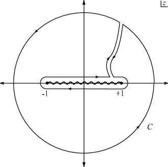
Figure 5: Contour $C$ in the complex $z$-plane used for the Nyquist analysis.

The last contribution can be evaluated using

$$\int_{-1+i\epsilon}^{1+i\epsilon}dz\frac{f^{\prime}_{\mp}(z)}{f_{\mp}(z)}=\ln\frac{f_{\mp}(1+i\epsilon)}{f_{\mp}(-1+i\epsilon)}+2\pi in\,\text{,}$$ (19)

for the line above and the corresponding expression for the line below the cut. $n$ is the number of times the function $f_{\mp}$ crosses the logarithmic cut located on the real axis, running from zero to minus infinity. This cut is due to the appearance of the logarithm on the right hand side of Eq. (19). In the sum of the line integrations above and below the cut diverging contributions from the first part on the right hand side of Eq. (19) cancel and we are left with a contribution of $2\pi i$ for each function. Furthermore it is necessary to show that neither $f_{-}$ nor $f_{+}$ crosses the cut. The proof is given in some detail for $f_{-}$ and is performed analogously for $f_{+}$. From Eq. (16) we find for $f_{-}$:

$$f_{-}(z,k,\xi) =z-1+\frac{\sqrt{1+\xi}}{2(1+\xi x^{2})}\frac{1}{k^{2}}\left[-2\left(z+\frac{1}{\xi}\right)\sqrt{\xi}\arctan\sqrt{\xi}+(z-1)\ln\left(\frac{z+1}{z-1}\right)\right]\,\text{.}$$ (20)

We want to study whether this function crosses the real axis in the range $\text{Re}[z]\in[-1,1]$ for $\text{Im}[z]\rightarrow 0$, i.e., whether the imaginary part of $f_{-}$ changes sign in that range. On the straight line infinitesimally above the cut the imaginary part of $f_{-}$ is given by

$$\text{Im}\left[\lim_{\epsilon\rightarrow 0}f_{-}(x+i\epsilon,k,\xi)\right]=-\frac{\pi}{2}\frac{\sqrt{1+\xi}(x-1)}{k^{2}(1+\xi x^{2})}\,\text{,}$$ (21)

for real $x$. It is only zero for $x=1$, which means that the function $f_{-}$ can not cross but merely touch the cut within the limits of the integration. On the straight line below the cut we get the same result (21) with a minus sign. For $f_{+}$, we find that the imaginary part in the regarded range only becomes zero for $x=-1$, which means that the logarithmic cut is not crossed within $[-1,1]$ either. Hence we have proved for the case $\mathbf{k}\parallel\mathbf{\hat{n}}$ that there are no more solutions than the four stable modes. In particular we have shown that unstable fermionic modes can not exist.

II.2 Large-$\xi$ limit

In the extremely anisotropic case where $\xi\rightarrow\infty$ the self-energies for arbitrary angle $\theta_{n}$ can be calculated explicitly. The distribution function (2) becomes Romatschke (2003)

$$\lim_{\xi\rightarrow\infty}f_{\xi}(\textbf{p})=\delta(\mathbf{\hat{p}}\cdot\mathbf{\hat{n}})\int_{-\infty}^{\infty}dxf_{\text{iso}}\left(p\sqrt{1+x^{2}}\right)\,\text{.}$$ (22)

With $\mathbf{\hat{n}}$ in the $z$-direction this implies that $\mathbf{p}$ lies in the $x$-$y$-plane only. As in Section II, due to azimuthal symmetry, we consider the case where $\mathbf{k}$ lies in the $x$-$z$-plane only. Using (22) we obtain from Eqs. (12)

$$\Sigma_{0}(\omega,k,\theta_{n}) =\frac{\pi}{2}m_{q}^{2}\frac{1}{\sqrt{\omega+k\sin\theta_{n}}\sqrt{\omega-k\sin\theta_{n}}}\,\text{,}$$

$$\Sigma_{x}(\omega,k,\theta_{n}) =\frac{\pi}{2k\sin\theta_{n}}m_{q}^{2}\left(\frac{\omega}{\sqrt{\omega+k\sin\theta_{n}}\sqrt{\omega-k\sin\theta_{n}}}-1\right)\,\text{.}$$ (23)

Since $p_{z}$ is always zero, $\Sigma_{z}$ vanishes. Eq. (11) now becomes

$$\omega-\Sigma_{0}=\pm\sqrt{(k_{x}-\Sigma_{x})^{2}+k_{z}^{2}}\,\text{.}$$ (24)

Nyquist analysis

Again, we only find four stable modes and will now show analytically that these are the only solutions in the large $\xi$-limit for arbitrary angle $\theta_{n}$. The cut resulting from the complex square roots in (23) can be chosen to lie between $z=-\sin\theta_{n}$ and $z=\sin\theta_{n}$ on the real axis. The Nyquist analysis can then be performed analogously to that in Section II.1 with the contour in Fig. 5 adjusted such that the inner path still runs infinitesimally close around the cut. Using this path in the evaluation of Eq. (17) for the functions

$$f_{\mp}(\omega,k,\theta_{n})=\omega-\Sigma_{0}\mp\sqrt{(k_{x}-\Sigma_{x})^{2}+k_{z}^{2}}\,\text{,}$$ (25)

we find the number of solutions to Eq. (24) to be

$$N_{\mp}=1+0+\frac{1}{4}+\frac{1}{4}+\frac{1}{2}=2\,\text{,}$$ (26)

so that again there are $N=N_{+}+N_{-}=4$ solutions, which are the known stable modes. The decomposition in (26) is done as follows:

1. The first contribution to $N_{\mp}$ comes from integration along the large outer circle at $|z|\gg 1$.

2. The zero stems from the paths connecting the outer and the inner circle.

3. The two contributions of $1/4$ result from integrations along the small circles around $-\sin\theta_{n}$ and $\sin\theta_{n}$.

4. The last contribution of $1/2$ comes from integration along the straight lines running infinitesimally close above and below the cut. We discuss this part in further detail below.

The last contribution can be obtained using Eq. (19). For the evaluation of the limit $\epsilon\rightarrow 0$ it is essential to note that the $f_{\mp}$ behave like $\ln\epsilon$ or $1/(\ln\epsilon)$ (depending on which function is evaluated on which line) and are both negative as $\epsilon\rightarrow 0$. This results in a contribution of $+i\pi$ for each function and integration, because in all cases the imaginary part of both functions can be shown to be positive in the regarded limit. All other contributions, including the diverging parts $\pm\ln(-\ln\epsilon)$ cancel in the sum of the results from the upper and lower line.

Again, we need to show that the functions $f_{\mp}$ do not cross the logarithmic cut for $z\in[-\sin\theta_{n},\sin\theta_{n}]$, i.e., that $n=0$ in Eq. (19). It is possible to find an analytic expression for the imaginary part of $f_{\mp}$ using

$$\text{Im}\sqrt{x+iy}=\frac{1}{\sqrt{2}}\,\text{sgn}(y)\sqrt{\sqrt{x^{2}+y^{2}}-x}\,\text{,}$$ (27)

for the imaginary part of the square root appearing in (25) with real $x$ and $y$. Then the only solutions to

$$\text{Im}f_{\mp}(z)=0$$ (28)

are found analytically to be $\text{Re}(z)=\sin\theta_{n}$ and $\text{Re}(z)=-\sin\theta_{n}$ for $f_{-}$ and $f_{+}$ respectively. This means that the cut is not crossed during the integration along the straight lines and that the contribution from this piece is in fact $1/2$.

III Fermion self-energy from the real-time formalism

In this section we extend our previous results to the real-time formalism and demonstrate that the high-temperature limit of the Kubo-Martin-Schwinger formula, $\Sigma_{12}=-\Sigma_{21}$, holds even for the non-equilibrium configuration considered here. We will use the real-time formulation of Refs. Schwinger (1961); Keldysh (1964, 1965); Chou et al. (1985); Landsman and van Weert (1987); Carrington et al. (1999). In this case both propagators and self-energies become $2\times 2$ matrices. The free propagators are given by

$$S(K)=(\not{K}+m) \left[\left(\begin{array}[]{cc}\frac{1}{K^{2}-m^{2}+i\epsilon}&0\\ 0&\frac{-1}{K^{2}-m^{2}-i\epsilon}\end{array}\right)\right.$$ (31)

$$~{}~{}~{}~{}~{}~{}\left.+2\pi i\delta(K^{2}-m^{2})\left(\begin{array}[]{cc}f_{\text{F}}(K)&-\theta(-k_{0})+f_{\text{F}}(K)\\ -\theta(k_{0})+f_{\text{F}}(K)&f_{\text{F}}(K)\end{array}\right)\right]\text{,}$$ (34)

with the general fermion distribution function $f_{\text{F}}(K)$.

The components $(12)$ and $(21)$ of the self-energy matrices are related to the emission and absorption probability of the particle species under consideration Chou et al. (1985); Mrowczynski and Heinz (1994); Calzetta and Hu (1988). To lowest order photons are produced via annihilation and Compton processes

$$q+\bar{q}\to g+\gamma,\qquad q(\bar{q})+g\to q(\bar{q})+\gamma\,.$$ (35)

Within the real-time formalism the rate of photon emission can be expressed as Baier et al. (1997b)

$$E\frac{dR}{d^{3}q}=\frac{i}{2(2\pi)^{3}}{\Pi_{12}}_{\mu}^{\mu}(Q)\,,$$ (36)

from the trace of the (12)-element $\Pi_{12}$ of the photon-polarization tensor.

$$-i{\Pi_{12}}_{\mu}^{\mu}(Q)=-e^{2}e_{q}^{2}N_{c}\int\frac{d^{4}p}{(2\pi)^{4}}Tr\left[\gamma^{\mu}\left.iS_{12}^{\star}(P)\right|_{HL}\gamma_{\mu}iS_{21}(P-Q)+\gamma^{\mu}iS_{12}(P)\gamma_{\mu}\left.iS_{21}^{\star}(P-Q)\right|_{HL}\right]\,,$$ (37)

where $e_{q}$ is the quark charge. Here $S_{12}$ and $S_{21}$ are the free fermion propagators from Eq. (34) and propagators with an HL subscript are the full propagators in the hard-loop approximation. The hard-loop propagators satisfy a fluctuation dissipation relation, which in the quasi-static case is given by

$$S_{12/21}^{\star}\left.(P)\right|_{HL}=\left.S_{\text{ret}}^{\star}(P)\right|_{HL}\Sigma_{12/21}(P)\left.S_{\text{adv}}^{\star}(P)\right|_{HL}\text{\,.}$$ (38)

The retarded propagator reads

$$\left.S_{\text{ret}}^{\star}(P)\right|_{HL}=\frac{1}{\not{P}-m-\Sigma(P)}\text{\,,}$$ (39)

where $\Sigma(P)$ is the retarded self-energy given in Eq. (1). The advanced propagator follows analogously with the advanced self-energy and to one loop order $\Sigma_{12}$ is given by

$$\Sigma_{12}(P)=2ig^{2}C_{\text{F}}\int\frac{d^{4}p}{(2\pi)^{4}}S_{12}(K)\Delta_{12}(Q)\text{\,,}$$ (40)

where $\Delta_{12}$ is the (12)-element of the matrix boson propagator given by

$$\Delta(K)=\left(\begin{array}[]{cc}\frac{1}{K^{2}-m^{2}+i\epsilon}&0\\ 0&\frac{-1}{K^{2}-m^{2}-i\epsilon}\end{array}\right)-2\pi i\delta(K^{2}-m^{2})\left(\begin{array}[]{cc}f_{\text{B}}(K)&\theta(-k_{0})+f_{\text{B}}(K)\\ \theta(k_{0})+f_{\text{B}}(K)&f_{\text{B}}(K)\end{array}\right)\text{\,.}$$ (45)

With the anisotropic distribution function (2) $\Sigma_{12}$ can be evaluated in the hard-loop approximation to read

$$\Sigma_{12}^{\mu}(P) = i\frac{g^{2}C_{\text{F}}}{(2\pi)^{2}}\int d\tilde{k}\int_{0}^{2\pi}d\phi\int_{-1}^{+1}dx\,\frac{\tilde{k}^{2}}{(1+\xi x^{2})^{3/2}}$$

$$\times\left[\!\left.\frac{k^{\mu}}{k}\right|_{k_{0}=k}\!\!\delta\left(g_{-}\right)N(\xi)f_{F}^{\text{iso}}(\tilde{k})\left(N(\xi)f_{\text{B}}^{\text{iso}}(\tilde{k})+1\right)+\left.\frac{k^{\mu}}{k}\right|_{k_{0}=-k}\!\!\delta\left(g_{+}\right)N(\xi)f_{B}^{\text{iso}}(\tilde{k})\left(N(\xi)f_{\text{F}}^{\text{iso}}(\tilde{k})-1\right)\!\right]\text{\,,}$$

where

$$g_{\pm}=2\frac{\tilde{k}}{\sqrt{1+\xi x^{2}}}\left[\pm p_{0}+p\left(\sin\theta_{n}\sqrt{1-x^{2}}\cos\phi+\cos\theta_{n}x\right)\right]$$ (47)

Figure 6: $\theta_{n}$-dependent part $\alpha^{0}$ of the self-energy $\Sigma_{12}^{0}$. $\theta_{n}\in\{0,\pi/4,\pi/2\}$ and $\xi=100$.

and we chose $\mathbf{p}$ to lie in the $x-z$-plane and used the change of variables (5) for $k$. Note that in the hard-loop limit one can ignore the quark masses and hence they have been explicitly set to zero above. The term $k^{\mu}/k$ does not depend on $k$ and is given by $(\pm 1,\sin\theta\cos\phi,\sin\theta\sin\phi,\cos\theta)$. Evaluation of the $\delta$-function leads to

$$-i\Sigma_{12}^{\mu}(P,\theta_{n},\xi)= A\,\alpha^{\mu}(P,\theta_{n},\xi)+B\,\beta^{\mu}(P,\theta_{n},\xi)\text{\,,}$$ (48)

with

$$\alpha^{\mu}(P,\theta_{n},\xi) =\int d\phi\,\sum_{i}\left.\frac{k^{\mu}}{k}\right|_{k_{0}=k}\left|\frac{(1-x_{i}^{2})^{1/2}}{(1-x_{i}^{2})^{1/2}(p\cos\theta_{n}+p_{0}\xi x_{i})-p\sin\theta_{n}x_{i}(1+\xi)\cos\phi}\right|\theta(1-x_{i}^{2})$$

$$\beta^{\mu}(P,\theta_{n},\xi) =\int d\phi\,\sum_{i}\left.\frac{k^{\mu}}{k}\right|_{k_{0}=-k}\left|\frac{(1-\tilde{x}_{i}^{2})^{1/2}}{(1-\tilde{x}_{i}^{2})^{1/2}(p\cos\theta_{n}-p_{0}\xi\tilde{x}_{i})-p\sin\theta_{n}\tilde{x}_{i}(1+\xi)\cos\phi}\right|\theta(1-\tilde{x}_{i}^{2})\text{\,,}$$ (49)

where the $x_{i}$ and $\tilde{x}_{i}$ are solutions to $\frac{\tilde{k}}{\sqrt{1+\xi x^{2}}}\left[-p_{0}+p\left(\sin\theta_{n}\sqrt{1-x^{2}}\cos\phi+\cos\theta_{n}x\right)\right]=0$ and $\frac{\tilde{k}}{\sqrt{1+\xi x^{2}}}\left[p_{0}+p\left(\sin\theta_{n}\sqrt{1-x^{2}}\cos\phi+\cos\theta_{n}x\right)\right]=0$, respectively, and

$$A =\frac{g^{2}C_{\text{F}}}{8\pi^{2}}\int dk\,k\,N(\xi)f_{F}^{\text{iso}}(k)\left(N(\xi)f_{\text{B}}^{\text{iso}}(k)+1\right)\text{\,,}$$ (50)

$$B =\frac{g^{2}C_{\text{F}}}{8\pi^{2}}\int dk\,k\,N(\xi)f_{B}^{\text{iso}}(k)\left(N(\xi)f_{\text{F}}^{\text{iso}}(k)-1\right)\text{\,.}$$ (51)

There can be $N\in\{0,1,2\}$ solutions for both $x_{i}$ and $\tilde{x}_{i}$, depending on the parameters $p,p_{0},\theta_{n}$ and $\phi$. Note that $\frac{k^{\mu}}{k}$ is also given in terms of the $x_{i}$. It is easily verified that

$$\alpha^{\mu}(P,\theta_{n},\xi)=-\beta^{\mu}(P,\theta_{n},\xi)\text{\,,}$$ (52)

Figure 7: $\theta_{n}$-dependent part $\alpha^{x}$ of the self-energy $\Sigma_{12}^{x}$. $\theta_{n}\in\{0,\pi/4,\pi/2\}$ and $\xi=100$. For $\theta_{n}=0$ $\alpha^{x}=0$.

Figure 8: $\theta_{n}$-dependent part $\alpha^{z}$ of the self-energy $\Sigma_{12}^{z}$. $\theta_{n}\in\{0,\pi/4,\pi/2\}$ and $\xi=100$. For $\theta_{n}=\pi/2$ $\alpha^{z}=0$.

such that Eq.  (48) greatly simplifies to read

$$-i\Sigma_{12}^{\mu}(P,\theta_{n},\xi)=(A-B)\,\alpha^{\mu}(P,\theta_{n},\xi)\text{\,,}$$ (53)

where

$$A-B={g^{2}C_{F}\over 8\pi^{2}}N(\xi)\left[\int_{0}^{\infty}dk\,k\,\left(f^{\rm iso}_{B}(k)+f^{\rm iso}_{F}(k)\right)\right]=\frac{1}{4}m_{q}^{2}N(\xi)\;,$$ (54)

assuming equal quark and antiquark distributions. We did not present the analogous explicit calculation of $\Sigma_{21}$, but find for it the same result as for $\Sigma_{12}$ with $A$ and $B$ interchanged. We also verified that $\Sigma_{12}$ and $\Sigma_{21}$ fulfill the general relation

$$\Sigma_{21}-\Sigma_{12}=2i\,\text{Im}\,\Sigma\text{\,,}$$ (55)

with the retarded self-energy $\Sigma$ given in Sec. II. Furthermore, since $\Sigma_{21}$ is given by Eq. (53) with $A$ and $B$ interchanged it follows within the hard-loop approximation that with the form of the anisotropic distribution function assumed here it always holds that

$$\Sigma_{12}=-\Sigma_{21}\text{\,,}$$ (56)

which can be seen as a high-temperature limit for the Kubo-Martin-Schwinger relation in equilibrium, but also holds for finite $\xi$ and hence for non-equilibrium. Eqs. (55) and (56) show that in order to calculate the hard-loop photon production rate from an anisotropic plasma one need only know the retarded self-energy. We plot the functions $\alpha$ for an anisotropy parameter of $\xi=100$ and different angles $\theta_{n}$ in Figs. 6, 7 and 8 to emphasize the strong angular dependence once more.

IV Conclusions

In this paper we have extended the exploration of the collective modes of an anisotropic quark-gluon plasma by studying the quark collective modes. Specifically, we derived integral expressions for the quark self-energy for arbitrary anisotropy and evaluate these numerically using the momentum-space rescaling introduced in previous papers. Using direct numerical calculation we found only real timelike fermionic modes and no unstable modes. Additionally using complex contour integration we have proven analytically in the cases (a) when the wave vector of the collective mode is parallel to the anisotropy direction with arbitrary oblate anisotropy and (b) for all angles of propagation in the limit of an infinitely oblate anisotropy that there are no fermionic unstable modes. Finally, we calculated the fermion self-energy of an anisotropic plasma in the real-time formalism and demonstrated that within the hard-loop approximation the high-temperature limit of the Kubo-Martin-Schwinger formula, $\Sigma_{12}=-\Sigma_{21}$, holds even for the non-equilibrium configuration considered here. This means that it suffices to only have the retarded self-energy $\Sigma$ in order to complete a calculation of photon production from an anisotropic plasma in the hard-loop framework. This calculation is currently underway Schenke and Strickland (2006).

Appendix A Small-$\xi$ limit

In the limit $\xi\rightarrow 0$ we can evaluate the quark self-energy in a power series in the anisotropy parameter $\xi$. To linear order in $\xi$ we obtain

$$\Sigma_{0} = \Sigma_{0}^{\rm iso}+{\xi\over 4}\left\{{z\over k}\left(3\cos 2\theta_{n}+1\right)+\Sigma_{0}^{\rm iso}\left[\cos 2\theta_{n}+1-(3\cos 2\theta_{n}+1)z^{2}\right]\right\},$$ (57)

$${\Sigma_{x}\over\sin\theta_{n}} = \Sigma_{s}^{\rm iso}+{\xi\over 12}\left\{{1\over k}\left(5\cos 2\theta_{n}+3\right)+3\Sigma_{s}^{\rm iso}\left[3\cos 2\theta_{n}+3-(5\cos 2\theta_{n}+3)z^{2}\right]\right\},$$ (58)

$${\Sigma_{z}\over\cos\theta_{n}} = \Sigma_{s}^{\rm iso}+{\xi\over 12}\left\{{1\over k}\left(5\cos 2\theta_{n}-1\right)+3\Sigma_{s}^{\rm iso}\left[3\cos 2\theta_{n}-1-(5\cos 2\theta_{n}-1)z^{2}\right]\right\},$$ (59)

where

$$\Sigma_{0}^{\rm iso} = {m_{q}^{2}\over 2k}\log{\omega+k\over\omega-k}\;,$$ (60)

$$\Sigma_{s}^{\rm iso} = {m_{q}^{2}\over k}\left({\omega\over 2k}\log{\omega+k\over\omega-k}-1\right)\;.$$ (61)

References

- Gyulassy and McLerran (2005) M. Gyulassy and L. McLerran, Nucl. Phys. A750, 30 (2005), eprint nucl-th/0405013.
- Gyulassy (2004) M. Gyulassy (2004), eprint nucl-th/0403032.
- Heinz and Kolb (2002) U. W. Heinz and P. F. Kolb (2002), eprint hep-ph/0204061.
- Heinz (2003) U. W. Heinz, Nucl. Phys. A721, 30 (2003), eprint nucl-th/0212004.
- Pisarski (1989) R. D. Pisarski, Phys. Rev. Lett. 63, 1129 (1989).
- Braaten and Pisarski (1990) E. Braaten and R. D. Pisarski, Nucl. Phys. B337, 569 (1990).
- Pisarski (1991) R. D. Pisarski, Nucl. Phys. A525, 175 (1991).
- Shuryak (1978) E. V. Shuryak, Phys. Lett. B78, 150 (1978).
- Kajantie and Miettinen (1981) K. Kajantie and H. I. Miettinen, Zeit. Phys. C9, 341 (1981).
- Halzen and Liu (1982) F. Halzen and H. C. Liu, Phys. Rev. D25, 1842 (1982).
- Kajantie and Ruuskanen (1983) K. Kajantie and P. V. Ruuskanen, Phys. Lett. B121, 352 (1983).
- Sinha (1983) B. Sinha, Phys. Lett. B128, 91 (1983).
- Hwa and Kajantie (1985) R. C. Hwa and K. Kajantie, Phys. Rev. D32, 1109 (1985).
- Staadt et al. (1986) G. Staadt, W. Greiner, and J. Rafelski, Phys. Rev. D33, 66 (1986).
- Neubert (1989) M. Neubert, Z. Phys. C42, 231 (1989).
- Kapusta et al. (1991) J. I. Kapusta, P. Lichard, and D. Seibert, Phys. Rev. D44, 2774 (1991).
- Baier et al. (1992) R. Baier, H. Nakkagawa, A. Niegawa, and K. Redlich, Z. Phys. C53, 433 (1992).
- Baier et al. (1994) R. Baier, S. Peigne, and D. Schiff, Z. Phys. C62, 337 (1994), eprint hep-ph/9311329.
- Aurenche et al. (1998) P. Aurenche, F. Gelis, R. Kobes, and H. Zaraket, Phys. Rev. D58, 085003 (1998), eprint hep-ph/9804224.
- Aurenche et al. (2000a) P. Aurenche, F. Gelis, and H. Zaraket, Phys. Rev. D61, 116001 (2000a), eprint hep-ph/9911367.
- Aurenche et al. (2000b) P. Aurenche, F. Gelis, and H. Zaraket, Phys. Rev. D62, 096012 (2000b), eprint hep-ph/0003326.
- Steffen and Thoma (2001) F. D. Steffen and M. H. Thoma, Phys. Lett. B510, 98 (2001), eprint hep-ph/0103044.
- Peitzmann and Thoma (2002) T. Peitzmann and M. H. Thoma, Phys. Rept. 364, 175 (2002), eprint hep-ph/0111114.
- Arnold et al. (2001a) P. Arnold, G. D. Moore, and L. G. Yaffe, JHEP 11, 057 (2001a), eprint hep-ph/0109064.
- Arnold et al. (2001b) P. Arnold, G. D. Moore, and L. G. Yaffe, JHEP 12, 009 (2001b), eprint hep-ph/0111107.
- Peitzmann (2003) T. Peitzmann, Pramana 60, 651 (2003), eprint nucl-ex/0201003.
- Arnold et al. (2003a) P. Arnold, G. D. Moore, and L. G. Yaffe, JHEP 01, 030 (2003a), eprint hep-ph/0209353.
- Shuryak and Xiong (1993) E. V. Shuryak and L. Xiong, Phys. Rev. Lett. 70, 2241 (1993), eprint hep-ph/9301218.
- Dumitru et al. (1993) A. Dumitru, D. H. Rischke, H. Stoecker, and W. Greiner, Mod. Phys. Lett. A8, 1291 (1993).
- Strickland (1994) M. Strickland, Phys. Lett. B331, 245 (1994).
- Traxler et al. (1995) C. T. Traxler, H. Vija, and M. H. Thoma, Phys. Lett. B346, 329 (1995), eprint hep-ph/9410309.
- Traxler and Thoma (1996) C. T. Traxler and M. H. Thoma, Phys. Rev. C53, 1348 (1996), eprint hep-ph/9507444.
- Kampfer and Pavlenko (1994) B. Kampfer and O. P. Pavlenko, Z. Phys. C62, 491 (1994).
- Srivastava et al. (1997) D. K. Srivastava, M. G. Mustafa, and B. Muller, Phys. Rev. C56, 1064 (1997), eprint nucl-th/9611041.
- Baier et al. (1997a) R. Baier, M. Dirks, and K. Redlich, Phys. Rev. D55, 4344 (1997a), eprint hep-ph/9610210.
- Baier et al. (1997b) R. Baier, M. Dirks, K. Redlich, and D. Schiff, Phys. Rev. D56, 2548 (1997b), eprint hep-ph/9704262.
- Mrowczynski (1993) S. Mrowczynski, Phys. Lett. B314, 118 (1993).
- Mrowczynski (1994) S. Mrowczynski, Phys. Rev. C49, 2191 (1994).
- Mrowczynski (1997) S. Mrowczynski, Phys. Lett. B393, 26 (1997), eprint hep-ph/9606442.
- Mrowczynski and Thoma (2000) S. Mrowczynski and M. H. Thoma, Phys. Rev. D62, 036011 (2000), eprint hep-ph/0001164.
- Birse et al. (2003) M. C. Birse, C.-W. Kao, and G. C. Nayak, Phys. Lett. B570, 171 (2003), eprint hep-ph/0304209.
- Randrup and Mrowczynski (2003) J. Randrup and S. Mrowczynski, Phys. Rev. C68, 034909 (2003), eprint nucl-th/0303021.
- Romatschke and Strickland (2003) P. Romatschke and M. Strickland, Phys. Rev. D68, 036004 (2003), eprint hep-ph/0304092.
- Arnold et al. (2003b) P. Arnold, J. Lenaghan, and G. D. Moore, JHEP 08, 002 (2003b), eprint hep-ph/0307325.
- Romatschke and Strickland (2004) P. Romatschke and M. Strickland, Phys. Rev. D70, 116006 (2004), eprint hep-ph/0406188.
- Mrowczynski et al. (2004) S. Mrowczynski, A. Rebhan, and M. Strickland, Phys. Rev. D70, 025004 (2004), eprint hep-ph/0403256.
- Dumitru and Nara (2005) A. Dumitru and Y. Nara, Phys. Lett. B621, 89 (2005), eprint hep-ph/0503121.
- Manuel and Mrowczynski (2005) C. Manuel and S. Mrowczynski, Phys. Rev. D72, 034005 (2005), eprint hep-ph/0504156.
- Arnold et al. (2005) P. Arnold, G. D. Moore, and L. G. Yaffe, Phys. Rev. D72, 054003 (2005), eprint hep-ph/0505212.
- Rebhan et al. (2005) A. Rebhan, P. Romatschke, and M. Strickland, JHEP 09, 041 (2005), eprint hep-ph/0505261.
- Romatschke and Venugopalan (2006a) P. Romatschke and R. Venugopalan, Phys. Rev. Lett. 96, 062302 (2006a), eprint hep-ph/0510121.
- Dumitru et al. (2006) A. Dumitru, Y. Nara, and M. Strickland (2006), eprint hep-ph/0604149.
- Schenke et al. (2006) B. Schenke, M. Strickland, C. Greiner, and M. H. Thoma, Phys. Rev. D 73, 125004 (2006), eprint hep-ph/0603029.
- Romatschke and Venugopalan (2006b) P. Romatschke and R. Venugopalan (2006b), eprint hep-ph/0605045.
- Romatschke and Rebhan (2006) P. Romatschke and A. Rebhan (2006), eprint hep-ph/0605064.
- Mrowczynski (2002) S. Mrowczynski, Phys. Rev. D65, 117501 (2002), eprint hep-ph/0112100.
- Stoof et al. (1996) H. Stoof, M. Houbiers, C. Sackett, and R. Hulet, Phys. Rev. Lett. 76, 10 (1996).
- Houbiers et al. (1997) M. Houbiers, R. Ferwerda, H. T. C. Stoof, W. I. McAlexander, C. A. Sackett, and R. G. Hulet, Phys. Rev. A 56, 4864 (1997).
- Holland et al. (2001) M. Holland, S. J. J. M. F. Kokkelmans, M. L. Chiofalo, and R. Walser, Phys. Rev. Lett. 87, 120406 (2001).
- Timmermans et al. (2001) E. Timmermans, K. Furuya, P. Milonni, and A. Kerman, Phys. Lett. A285, 228 (2001).
- Ohashi and Griffin (2002) Y. Ohashi and A. Griffin, Phys. Rev. Lett. 89, 130402 (2002).
- Kinast et al. (2004) J. Kinast, S. Hemmer, M. Gehm, A. Turlapov, and J. Thomas, Phys. Rev. Lett. 92, 150402 (2004).
- Romatschke (2003) P. Romatschke, Ph.D. thesis (2003), eprint hep-ph/0312152.
- Schwinger (1961) J. S. Schwinger, J. Math. Phys. 2, 407 (1961).
- Keldysh (1964) L. Keldysh, Zh. Eks. Teor. Fiz. 47, 1515 (1964).
- Keldysh (1965) L. Keldysh, Sov. Phys. JETP 20, 1018 (1965).
- Chou et al. (1985) K.-c. Chou, Z.-b. Su, B.-l. Hao, and L. Yu, Phys. Rept. 118, 1 (1985).
- Landsman and van Weert (1987) N. P. Landsman and C. G. van Weert, Phys. Rept. 145, 141 (1987).
- Carrington et al. (1999) M. E. Carrington, D.-f. Hou, and M. H. Thoma, Eur. Phys. J. C7, 347 (1999), eprint hep-ph/9708363.
- Mrowczynski and Heinz (1994) S. Mrowczynski and U. W. Heinz, Ann. Phys. 229, 1 (1994).
- Calzetta and Hu (1988) E. Calzetta and B. L. Hu, Phys. Rev. D37, 2878 (1988).
- Schenke and Strickland (2006) B. Schenke and M. Strickland, forthcoming (2006).