Compatibility of CAST search with axion-like interpretation of PVLAS results

Abstract

The PVLAS collaboration has results that may be interpreted in terms of a light axion-like particle, while the CAST collaboration has not found any signal of such particles. We propose a particle physics model with paraphotons and with a low energy scale in which this apparent inconsistency is circumvented.

Very recently, the PVLAS collaboration has announced the observation of a rotation of the plane of polarization of laser light propagating in a magnetic field Zavattini:2005tm . This dichroism of vacuum in magnetic fields may be explained as the oscillation of photons into very light particles $\phi$. If true, this would be of course a revolutionary finding nature .

The lagrangian that would describe the necessary $\phi\gamma\gamma$ coupling is

$${\cal L}_{\phi\gamma\gamma}=\frac{1}{8M}\,\epsilon_{\mu\nu\rho\sigma}F^{\mu\nu}{F}^{\rho\sigma}\,\phi$$ (1)

when $\phi$ is a pseudoscalar, and when it is a scalar is

$${\cal L}_{\phi\gamma\gamma}=\frac{1}{4M}\,F^{\mu\nu}F_{\mu\nu}\,\phi$$ (2)

with $F^{\mu\nu}$ the electromagnetic field tensor. We shall refer to $\phi$ in both cases as an axion-like particle (ALP). Let us remark that a transition to a spin-two particle contributes to the polarization rotation negligibly Biggio:2006im .

Either (1) or (2) lead to $\gamma-\phi$ mixing in a magnetic field and, if $\phi$ is light enough, to coherent transitions that enhance the signal Maiani:1986md . Interpreted in these terms, the PVLAS observation Zavattini:2005tm leads to a mass for the ALP

$$1\ {\rm meV}\lesssim m_{\phi}\lesssim 1.5\ {\rm meV}$$ (3)

and to a coupling strength corresponding to

$$2\times 10^{5}\ {\rm GeV}\lesssim M\lesssim 6\times 10^{5}\ {\rm GeV}\ \ \ .$$ (4)

Of course we would like to have an independent test of such an interpretation. There are ongoing projects that will in the near future probe $\gamma-\phi$ transitions ringwald . In the meanwhile we should face the problem of the apparent inconsistency between the value (4) and other independent results, namely, the CAST observations Zioutas:2004hi on the one hand, and the astrophysical bounds on the coupling of ALPs to photons on the other hand Raffelt:1996wa .

The CAST collaboration has recently published Zioutas:2004hi a limit on the strength of (1) or (2). A light particle coupled to two photons would be produced by Primakoff-like processes in the solar core. CAST is an helioscope Sikivie:1983ip that tries to detect the $\phi$ flux coming from the Sun, by way of the coherent transition of $\phi$’s to X-rays in a magnetic field. As no signal is observed they set the bound

$$M>0.87\times 10^{10}\ {\rm GeV}\ \ \ ,$$ (5)

which is in strong disagreement with (4).

Also, the production of $\phi$’s in stars is constrained because too much energy loss in exotic channels would lead to drastic changes in the timescales of stellar evolution. Empirical observations of globular clusters place a bound Raffelt:1996wa , again in contradiction with (4),

$$M>1.7\times 10^{10}\ {\rm GeV}\ \ \ .$$ (6)

As it has been stressed in Masso:2005ym , once we are able to relax (6) we could also evade (5). Indeed, the CAST bound assumes standard solar emission. From the moment we alter the standard scenario we should revise (5). In Masso:2005ym ; Jain:2005nh ; Jaeckel:2006id two ideas on how to evade the astrophysical bound (6) are presented. One possibility is that the produced ALPs diffuse in the stellar medium, so that they are emitted with much less energy than originally produced Masso:2005ym . A second possibility is that the production of ALPs is much less than expected because there is a mechanism of suppression that acts in the stellar conditions. We will present in this letter a paraphoton model with a low energy scale where the particle production in stars is suppressed enough to accommodate both the CAST and the PVLAS results.

I Triangle diagram and epsilon-charged particles

The physical idea beyond this letter is that to understand PVLAS and CAST in an ALP framework we have to add some new physics structure to the vertices (1),(2). The scale of the new physics should be much less than O(keV), the typical temperature in astrophysical environments.

We will assume that this structure is a simple loop where a new fermion $f$ circulates; see Fig.(1). The amplitude of the $\phi\gamma\gamma$ diagram can be easily calculated and identified with the coefficient in (1) or (2)

$$\frac{1}{M}=\frac{\alpha}{\pi}\frac{q_{f}^{2}}{v}$$ (7)

Here $\alpha=e^{2}/4\pi$, and the charge of the fermion $f$ is $eq_{f}$. The value of the mass-scale $v$ depends on the $\phi\bar{f}f$ vertex. If $\phi$ is a pseudoscalar $v_{\rm PS}=m_{f}/g_{\rm PS}$ while if is scalar $v_{\rm S}=f(m_{f},m_{\phi})$ not far from $v_{\rm S}\sim m_{f}\sim m_{\phi}$ if $m_{f}\sim m_{\phi}$. Finally if $\phi$ is a Goldstone boson $v_{\rm GB}$ is related to the scale of breaking of the related global symmetry.

Figure 1: Triangle diagram for the $\phi\gamma\gamma$ vertex.

From (7) we see that $M$, the high energy scale (4), is connected to $v$. As we need $v$ to be a low energy scale, $q_{f}$ should be quite small.

Paraphoton models Holdom:1985ag naturally incorporate small charges. These models are QED extensions with extra $U(1)$ gauge bosons. A small mixing among the kinetic terms of the gauge bosons leads to the exciting possibility that paracharged exotic particles end up with a small induced electric charge Holdom:1985ag .

Getting a small charge for $f$ is not enough for our purpose since we need also production suppression of exotic particles in stellar plasmas. With this objective, we will present a model containing two paraphotons; if we allow for one of the paraphotons to have a mass, we will see we can evade the astrophysical constraints and consequently the model will be able to accommodate all experimental results. We describe it in what follows.

II A model with two paraphotons

Let us start with the photon part of the QED lagrangian,

$${\cal L}_{0}=-\frac{1}{4}F_{0}^{\mu\nu}F_{0\mu\nu}+e\ j_{0\mu}A_{0}^{\mu}$$ (8)

where $j_{0\mu}$ is the electromagnetic current involving electrons, etc., $j_{0\mu}\sim\bar{e}\gamma_{\mu}e+...$. From the $U_{0}(1)$ gauge symmetry group, we give the step of assuming $U_{0}(1)\times U_{1}(1)\times U_{2}(1)$ as the gauge symmetry group, with the corresponding gauge fields $A_{0}$, $A_{1}$, and $A_{2}$. With all generality there will be off-diagonal kinetic terms in the lagrangian, like $\epsilon_{01}\,F_{0}F_{1}$ and $\epsilon_{02}F_{0}F_{2}$ (Lorenz index contraction is understood). We expect these mixings to be small if we follow the idea in Holdom:1985ag that ultramassive particles with 0,1,2 charges running in loops are the responsibles for them. We will assume that these heavy particles are degenerate in mass and have identical 1 and 2 charges so that they induce identical mixings $\epsilon_{01}=\epsilon_{02}\equiv\epsilon$.

To write the complete lagrangian we use the matrix notation $A\equiv(A_{0},A_{1},A_{2})^{T}$ and $F\equiv(F_{0},F_{1},F_{2})^{T}$,

$${\cal L}=-\frac{1}{4}\,F^{T}{\cal M}_{F}\,F+\frac{1}{2}\,A^{T}{\cal M}_{A}\,A+e\sum_{i}\,j_{i}A_{i}$$ (9)

We call $A_{0}$, $A_{1}$, and $A_{2}$ interaction fields because the interaction term in (9) is diagonal, i.e. the interaction photon is defined to couple directly only to standard model particles. Here the kinetic matrix contains the mixings,

$${\cal M}_{F}=\left(\begin{array}[]{ccc}1&\epsilon&\epsilon\\ \epsilon&1&0\\ \epsilon&0&1\end{array}\right)$$ (10)

In general the diagonal terms are renormalized, $1\rightarrow 1+\delta$, and there are terms ${\cal M}_{F12}$. However, they do not play any relevant role here and we omit them.

As said, we need one of the paraphotons to be massive but it will prove convenient to work with a general ${\cal M}_{A}={\rm Diag}\,\{m_{0}^{2},m_{1}^{2},m_{2}^{2}\}$. Also, in the last term of (9) we see the currents $j_{1}$ and $j_{2}$ containing the paracharged exotic particles. To reduce the number of parameters we have set the unit paracharge equal to the unit of electric charge, so that there is a common factor $e$.

Diagonalization involves first a non-unitary reabsorption of the $\epsilon$ terms in (10) to have the kinetic part in the lagrangian in the canonical form, $(-1/4)F^{T}F$. After this, we diagonalize the mass matrix with a unitary transformation that maintains the kinetic part canonical ending up with the propagating field basis $\widetilde{A}$. We have $A={\cal U}\widetilde{A}$, with

$${\cal U}=\ \left(\begin{array}[]{ccc}1&\epsilon\,\frac{m_{1}^{2}}{m_{0}^{2}-m_{1}^{2}}&\epsilon\,\frac{m_{2}^{2}}{m_{0}^{2}-m_{2}^{2}}\\ \epsilon\,\frac{m_{0}^{2}}{m_{1}^{2}-m_{0}^{2}}&1&0\\ \epsilon\,\frac{m_{0}^{2}}{m_{2}^{2}-m_{0}^{2}}&0&1\end{array}\right)$$ (11)

We see that the interacting and the propagating photon differ by little admixtures of $O(\epsilon)$. (We work at first order in $\epsilon$).

We have developed a quite general two paraphoton model. The specific model we adopt has the following characteristics. First, only one paraphoton has a mass, say $m_{1}\equiv\mu\neq 0$, and $m_{2}=0$. Second, in order to get the effects we desire we have to assign opposite 1 and 2 paracharges to $f$, so that the interaction for $f$ appearing in the last term of (9) is

$$e\,\bar{f}\gamma_{\mu}f\,(A_{1}^{\mu}-A_{2}^{\mu})$$ (12)

Let us show why we choose these properties. The coupling of $f$ to photons in the interaction basis is shown in Fig.(2).

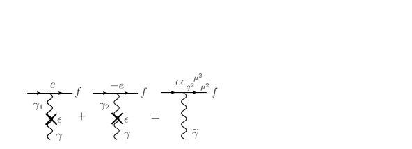
Figure 2: Diagrams of the interaction of $f$ with photons.

It proceeds through both paraphotons, with a relative minus sign among the two diagrams due to the assignment (12). The induced electric $f$ charge is thus

$$q_{f}={\cal U}_{10}-{\cal U}_{20}$$ (13)

We see from (11) that $m_{2}=0$ implies ${\cal U}_{20}=-\epsilon$. However, the value for ${\cal U}_{10}$ has to be discussed separately in the vacuum and the plasma cases. In vacuum, we have $m_{0}=0$, so that ${\cal U}_{10}=0$ and thus $q_{f}=\epsilon$. In this case $A_{0}$ and $A_{2}$ are degenerate and we can make arbitrary rotations in their sector. This corresponds to different charge assignments that of course leave the physics unchanged. Due to our method of handling the diagonalizations, eq.(11) is bad behaved for $m_{0}=m_{2}$, except for the case of our interest, $m_{0}=m_{2}=0$, in which the order in which we take the limits $m_{0}\rightarrow 0$ and $m_{2}\rightarrow 0$ gives different charge assignments according to the rotational freedom. Here we have made $m_{2}\rightarrow 0$ before $m_{0}\rightarrow 0$ to provide f with a milielectric charge as in Holdom:1985ag . Changing the order of the limits would end with a paracharge to electrons.

In the classical and non-degenerated plasmas we consider the dispersion relation can be taken as $k^{2}=\omega_{P}^{2}=4\pi\alpha n_{e}/m_{e}$ ($n_{e}$ and $m_{e}$ are the density and mass of electrons). If $m_{0}=\omega_{P}$ is much greater that $m_{1}=\mu$ we get ${\cal U}_{01}\simeq-\epsilon+\epsilon m_{1}^{2}/m_{0}^{2}$ and the induced electric charge

$$q_{f}(k^{2}\simeq\omega_{P}^{2})\,\simeq\,\frac{\mu^{2}}{\omega_{P}^{2}}\ q_{f}(k^{2}\simeq 0)\ \ \ .$$ (14)

Provided we have a low energy scale $\mu\ll\omega_{P}\sim$ keV, we reach our objective of having a strong decrease of the $f$ charge in the plasma, i.e., $q_{f}(\omega_{P}^{2})\ll q_{f}(0)=\epsilon$.

The cancelation of the two diagrams of Fig.2 requires that the equality $e_{1}=e_{2}$ holds up to terms of order $O(\mu^{2}/\omega^{2}_{P})$. Note that even if $e_{1}=e_{2}$ at some high energy scale because of a symmetry, a difference in the beta functions could also spoil our mechanism at low energy. The parafermion $f$ contributes equally to both beta functions so the problem are the contributions from the sector that gives mass only to $A_{1}$. However these contributions can be made arbitrarily small by sending the Higgs mass to infinity in the spirit of the non-linear realizations of symmetry breaking, by considering Higgsless models like breaking the symmetry geometrically, or by considering gauge coupling unification $e_{1}=e_{2}$ at an energy not far from the typical solar temperature. A further possibility is to consider $e_{1}=e_{2}\ll e$ which would suppress the loop-induced effects at the prize of making the model less natural.

III The role of the low-energy scale

We now discuss the consequences of our model. The PVLAS experiment is in vacuum, so $f$ has an effective electric charge $q_{f}(0)=\epsilon$, which from (7) has to be

$$\epsilon^{2}\simeq 10^{-12}\,\frac{v}{\rm eV}$$ (15)

Concerning the astrophysical constraints, we notice that the amplitude for the Primakoff effect $\gamma Z\rightarrow\phi Z$ is of order $q_{f}^{2}=\epsilon^{2}$ and that there are production processes with amplitudes of order $\epsilon$ which will be more effective. One is plasmon decay $\gamma^{*}\rightarrow\bar{f}f$. Energy loss arguments in horizontal-branch (HB) stars Davidson:1991si limits $q_{f}$ to be below $2\times 10^{-14}$, which translates in our model into the bound

$$\epsilon\ \frac{\mu^{2}}{\rm eV^{2}}<4\times 10^{-8}$$ (16)

(we have used $\omega_{P}\simeq 2$ keV in a typical HB core). Other processes like bremsstrahlung of paraphotons give weaker constraints.

Equations (15) and (16) do not fully determine the parameters of our model. Together they imply the constraint

$$v\,\mu^{4}<(\,0.4\ {\rm eV})^{5}$$ (17)

We can now make explicit one of our main results. In the reasonable case that $v$ and $\mu$ are not too different, we wee that the new physics scale is in the sub eV range.

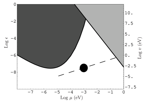
Figure 3: Constraints on the parameters of our model. The black area is excluded by Cavendish-type experiments, and the grey area by the astrophysical constraint (15). The dashed line corresponds to $v=\mu$, and the dot to $v=\mu\simeq 1$ meV.

Let us consider now the CAST limit.The CAST helioscope looks for $\phi$’s with energies within a window of 1-15 keV. In our model, $f$’s and paraphotons are emitted from the Sun, but we should watch out $\phi$ production. This depends on the specific characteristics of $\phi$. We consider three possibilities. A) $\phi$ is a fundamental particle. As we said the Primakoff production is very much suppressed, so production takes place mainly through plasmon decay $\gamma^{*}\rightarrow\bar{f}f\phi$. The $\phi$-flux is suppressed, but, most importantly, the average $\phi$ energy is much less than $\omega_{P}\simeq.3$ keV, the solar plasmon mass. The spectrum then will be below the present CAST energy window. B) $\phi$ is a composite $\bar{f}f$ particle confined by new strong confining forces. The final products of plasmon decay would be a cascade of $\phi$’s and other resonances which again would not have enough energy to be detected by CAST. C) $\phi$ is a positronium-like bound state of $\bar{f}f$, with paraphotons providing the necessary binding force. As the binding energy is necessarily small, ALPs are not produced in the solar plasma.

Let us now turn our attention to other constraints. Laboratory bounds on epsilon-charged particles are much milder than the astrophysical limits, as shown in Davidson:1991si . In our model, however, even though paraphotons do no couple to bulk electrically neutral matter, a massive paraphoton $\widetilde{A}_{1}$ couples to electrons with a strength $\epsilon$ and a range $\mu^{-1}$. This potential effect is limited by Cavendish type experiments Bartlett:1988yy .

In Fig.(3) we show these limits, as well as the astrophysical bound (16). In the ordinates we can see both $\epsilon$ and $v$, since we assume they are related by (15). At the view of the figure, we find out that there is wide room for the parameters of our model. However we would like that $v$ and $\mu$ do not differ too much among them. We display the line $v=\mu$, the region where this kind of naturality condition is fulfilled. The most economical version of the model would be obtained when the new scales are, on the order of magnitude, about the scale of the ALP mass of O(1 meV), (3). We have also indicated this privileged point in the parameter space.

Also, we should discuss cosmological constraints, i.e. production of paraphotons and $f$’s in the early universe. Taking into account that the vertices have suppression factors in the high temperatures of such environment, we find that there is not a relic density of any of them.

Finally, let us come back to the physics responsible for the $A_{1}$ mass. If this comes from an abelian Higgs mechanism then the Higgs boson acquires a milicharge $\varepsilon e_{1}$ and could be produced in the Sun and in the early universe, particularly in the period of primordial nucleosynthesis. However, this is not a problem if the mass of the Higgs is large enough, a constraint that we required at the end of section I when discussing charge running.

IV Conclusions

We have presented a model of new physics containing a paracharged particle $f$ and two paraphotons, one of which has a mass $\mu$ that sets the low energy scale of the model. With convenient assignments of the $f$ paracharges and mixings, we get an induced epsilon-charge for $f$ that moreover decreases sharply in a plasma with $\omega_{P}\gg\mu$. Our model accommodates an axion-like particle with the properties (3) and (4), able to explain the PVLAS results, while at the same time consistent with the astrophysical and the laboratory constraints, including the limit obtained by CAST.

We have some freedom in the parameter space of our model; however if we wish that the energy scales appearing in it are not too different, we are led to scales in the sub eV range. A preferred scale is O(meV), because then it is on the same order than the axion-like particle mass.

If the interpretation of the PVLAS experiment is confirmed, which means the exciting discovery of an axion-like particle, then to make it compatible with the CAST results and with the astrophysical bounds requires further new physics. In our model, the scale of this new physics is below the eV.

Note added: Recently, a paper has appeared ringstring that justifies our model in the context of string theory.

V acknowledgments

We acknowledge support by the projects FPA2005-05904 (CICYT) and 2005SGR00916 (DURSI).

References

- (1) E. Zavattini et al. [PVLAS Collaboration], Phys. Rev. Lett. 96, 110406 (2006) [arXiv:hep-ex/0507107].
- (2) S. Lamoreaux, Nature 441, 31 (2006).
- (3) C. Biggio, E. Masso and J. Redondo, arXiv:hep-ph/0604062.
- (4) L. Maiani, R. Petronzio and E. Zavattini, Phys. Lett. B 175, 359 (1986).
- (5) See for example the talk of A. Ringwald in http://www.desy.de/ringwald/axions/talks/patras.pdf
- (6) K. Zioutas et al. [CAST Collaboration], Phys. Rev. Lett. 94, 121301 (2005) [arXiv:hep-ex/0411033].
- (7) For a complete description see: G. G. Raffelt, Stars as laboratories for fundamental physics, Chicago Univ. Pr. (1996).
- (8) P. Sikivie, Phys. Rev. Lett. 51, 1415 (1983) [Erratum-ibid. 52, 695 (1984)].
- (9) G. G. Raffelt, arXiv:hep-ph/0504152.
- (10) E. Masso and J. Redondo, JCAP 0509, 015 (2005) [arXiv:hep-ph/0504202].
- (11) P. Jain and S. Mandal, arXiv:astro-ph/0512155.
- (12) J. Jaeckel, E. Masso, J. Redondo, A. Ringwald and F. Takahashi, arXiv:hep-ph/0605313.
- (13) B. Holdom, Phys. Lett. B 166, 196 (1986), ibid. 178, 65 (1986); L. B. Okun, Sov. Phys. JETP 56, 502 (1982) [Zh. Eksp. Teor. Fiz. 83, 892 (1982)].
- (14) S. Davidson, B. Campbell and D. Bailey, Phys. Rev. D 43, 2314 (1991); S. Davidson and M. Peskin, Phys. Rev. D 49, 2114 (1994) [arXiv:hep-ph/9310288]; S. Davidson, S. Hannestad and G. Raffelt, JHEP 0005, 003 (2000) [arXiv:hep-ph/0001179].
- (15) E. R. Williams, J. E. Faller and H. A. Hill, Phys. Rev. Lett. 26, 721 (1971); D. F. Bartlett and S. Logl, Phys. Rev. Lett. 61, 2285 (1988).
- (16) S. A. Abel, J. Jaeckel, V. V. Khoze, and A. Ringwald, [hep-ph/0608248].