1 Introduction

Supersymmetric theories contain a number of possible sources of lepton flavour violation. As a result, the bounds on rates of LFV and FCNC are particularly restricting upon the SUSY parameter space. Even in the case of minimal supergravity(mSUGRA), where soft SUSY breaking masses and trilinear couplings are flavour diagonal at the GUT scale, the presence of right-handed neutrinos and the PMNS mixings are enough to radiatively induce large LFV rates. It is these LFV rates, induced by renormalisation group(RG) running that we wish to study in the present work.

A large value of $\tan\beta$ enhances LFV and FCNC effects in SUSY theories and it is interesting to study them together within a SUSY-GUT scenario. In the large $\tan\beta$ limit it has been noted that Higgs mediated contributions to FCNC decays may be dominant. The most interesting example of Higgs mediated decays is that of $B^{0}_{s}\to\mu^{+}\mu^{-}$[2, 1] in the MSSM. This decay is proportional to $\tan^{6}\beta$ and so is greatly enhanced by large values of $\tan\beta$. If the Higgs boson is very light then this rate could become very exciting. Another interesting case is the Higgs mediated contribution to the recently measured $B_{s}^{0}\!-\!\bar{B}_{s}^{0}$ mixing at the Tevatron. Along with improved bounds on leptonic $B_{s}$ decays these measurements add a complimentary $b-s$ constraint to that of $b\to s\gamma$.

We propose to study the rates of lepton flavour violating decays of $\tau$, $B_{s}^{0}$ and MSSM neutral Higgs bosons in a SUSY-seesaw model with bi-large neutrino mixing. From this framework we hope to make general predictions for some of the interesting lepton flavour violating decays mentioned above and also to study their correlations. The present work differs from previous studies in that it makes use of a top-down $\chi^{2}$ analysis of a Grand Unified SUSY model. Also we are studying lepton flavour violating Higgs decays in conjunction with Higgs mediated decays, such as $B_{s}\to\mu^{+}\mu^{-}$.

2 A large $\tan\beta$ SUSY-seesaw model

In the present work we shall study the MSSM$+\nu_{R}$ constrained at the GUT scale by minimal $SU(5)$ unification. In Minimal $SU(5)$ the matter superfields of the MSSM$+\nu_{R}$ are contained within the representations; ${\bf 10}=(Q,\,U^{c},\,E^{c})$, and ${\bf\bar{5}}=(L,\,D^{c})$ and ${\bf 1}=(N^{c})$. In addition there are ${\bf 5}=\left(H_{u},\,H_{c}\right)$ and ${\bf\bar{5}}=\left(H_{d},\,\bar{H}_{c}\right)$ Higgs representations. Using these matter superfields we can construct the Yukawa section of the superpotential as follows,

$$W_{Y}^{SU(5)}=\frac{1}{8}\,Y_{u}^{ij}\,{\bf 10}_{i}{\bf 10}_{j}{\bf H}+Y_{d}^{ij}\,{\bf 10}_{i}{\bf\bar{5}}_{j}{\bf\bar{H}}+Y_{\nu}^{ij}\,{\bf\bar{5}}_{i}{\bf 1}_{j}{\bf H}+\frac{1}{2}\,M_{R}^{ij}\,{\bf 1}_{i}{\bf 1}_{j}.$$ (1)

The first term of eq. (1) gives rise to a symmetric up-quark Yukawa coupling $Y_{u}$ and the second term provides both down-quark and charged lepton Yukawa couplings. As a result we have the GUT scale relation, $Y_{e}=Y_{d}^{\sf T}$. The final two terms of eq. (1) are responsible for the neutrino Yukawa coupling, $Y_{\nu}$ and the right-handed neutrino Majorana mass, $M_{R}$ which combine to produce the light neutrino mass matrix via the type I seesaw mechanism,

$$m_{LL}=-\,v_{u}^{2}\,\,Y_{\nu}\,M_{R}^{-1}\,Y_{\nu}^{\sf T}.$$ (2)

We begin by rotating the ${\bf 10}$ and ${\bf\bar{5}}$ representations such that $Y_{d}$ is diagonal. As a result $Y_{u}$ is solely responsible for the CKM mixing. The lepton sector is more complicated due to the structure of the see-saw mass matrix eq. (2). Hence, in this basis we have,

$$Y_{u} = V_{\sf CKM}^{\sf T}\,Y_{u}^{\sf diag}\,V_{\sf CKM}$$

$$Y_{d} = Y_{d}^{\sf diag}$$

$$Y_{\nu} = U\,Y_{\nu}^{\sf diag}$$ (3)

$$M_{R} = W\;M_{R}^{\sf diag}\;W^{\sf T}.$$

Here the singlet neutrino has been rotated such that the combination, $Y_{\nu}^{\sf T}Y_{\nu}$, is diagonal. In the case were, $W=1$, the mixing matrix $U$ is identified as the PMNS matrix. Such a case may occur naturally, for example in models with a $U(1)_{X}$ flavour symmetry. For simplicity we assumed $W=1$ and that the above matrices are all real.

Throughout the analysis it was assumed that both the neutrino Yukawa and Majorana matrices have a hierarchical form with $Y_{\nu_{3}}^{\sf diag}\sim 1$ and $M_{R_{3}}\sim 10^{14}$ GeV, as shown in eq. (4) and (5). We choose such a hierarchy in the neutrino Yukawa sector with one eye on $b-t-\tau$ Yukawa unification and $SO(10)$ with $\tan\beta\sim 50$.

$$Y_{\nu_{1}}^{\sf diag}<Y_{\nu_{2}}^{\sf diag}<Y_{\nu_{3}}^{\sf diag}\sim 1$$ (4)

$$M_{R_{1}}^{\sf diag}<M_{R_{2}}^{\sf diag}<M_{R_{3}}^{\sf diag}\sim 10^{14}\,\,{\rm GeV}$$ . (5)

This hierarchy results in a neutrino mass ordering which is of the Normal Hierarchical type with, $m_{\nu_{1}}\approx 0.55\times 10^{-6}$ eV, $m_{\nu_{2}}\approx 0.009$ eV, $m_{\nu_{3}}\approx 0.05$ eV.

The consequence of our choice of $\lambda_{\nu_{3}}\sim 1$ is that it shall induce, via RG evolution, large flavour mixing in the slepton mass squared matrix. This slepton flavour mixing leads to a lepton-slepton mis-alignment and produces lepton flavour violation in the charged lepton sector. The choice of a large neutrino yukawa coupling enhances this effect and will result in a large rate for $\tau\to\mu\gamma$. It should be noted that such a large neutrino yukawa coupling is inevitable in models based on $SO(10)$.

In the soft SUSY breaking section of the Lagrangian flavour blind boundary conditions are assumed at the GUT scale. In this work we are interested in the renormalisation group effects of off-diagonal elements of the Yukawa couplings as discussed above. Due to the large mixings in the PMNS matrix, these off-diagonal elements can be large even in the case of GUT scale flavour blindness. Throughout our analysis we have also assumed that the trilinear coupling, $A_{0}=0$, at the GUT scale. Under these assumptions the soft Lagrangian becomes flavour blind and hence contains no new lepton flavour violating sources.

3 LFV and FCNC Phenomenology

Observations of neutrino oscillations imply the existence of massive neutrinos with large solar and atmospheric mixing angles. The small neutrino masses are most naturally explained via the seesaw mechanism with heavy singlet neutrinos. Even in a basis where both $Y_{e}$ and $M_{R}$ are diagonal in flavour space $Y_{\nu}$ is always left as a possible source of flavour violation. In SUSY models this flavour violation can be communicated to the slepton sector through renormalisation group running. The initial communication is from running between the GUT scale and the scale of $M_{R}$. Although the scale $M_{R}$ is far above the electro-weak scale its effects leave a lasting impression on the mass squared matrices of the sleptons. Subsequently flavour violation can enter into the charged lepton sector through loop diagrams involving the sleptons and indeed such effects have been used to predict large branching ratios for $\tau\to\mu\gamma$ and $\mu\to e\gamma$ within the MSSM [5, 6, 7, 8]. As such, the experimental bound on charged lepton flavour violation provide important constraints on the possible flavour mixing of the MSSM and other extensions of the SM.

In the Standard Model FCNCs are absent at tree-level and only enter at 1-loop order. In extensions of the SM, the MSSM for example, there also exist additional sources of FCNC. A clear example comes from the mixings present in the squark sector of the MSSM. These mixings will also contribute to FCNCs at the 1-loop level and could even be larger than their SM counterparts. An example that we shall study in this work is the flavour changing couplings of neutral Higgs bosons and the neutral Higgs penguin contribution to such decays as $B_{s}^{0}\to\mu^{+}\mu^{-}$ and $B_{s}^{0}\!-\!\bar{B}_{s}^{0}$ mixing. When examining such flavour changing in the quark sector it is important to consider the constraint imposed by the decay $b\to s\gamma$.

3.1 Higgs mediated FCNC

It has been pointed out that Higgs mediated FCNC processes could be among the first signals of supersymmetry[2]. In the MSSM radiatively induced couplings between the up Higgs, $H_{u}$, and down-type quarks may result in flavour changing Higgs couplings. In turn this will lead to large FCNC decay rates for such process as $B_{s}\to\mu^{+}\mu^{-}$ and $B_{s}^{0}\!-\!\bar{B}_{s}^{0}$ mixing. In the Standard Model the predicted branching ratio for $B_{s}\to\mu^{+}\mu^{-}$ is of the order of $10^{-9}$, but in the MSSM such a decay is enhanced by large $\tan\beta$ and may reach far greater rates. It is also possible to extend this picture to the charged lepton sector where similar lepton flavour violating higgs couplings are radiatively induced. These LFV couplings can then result in such Higgs mediated decays as $\tau\to 3\mu$, the neutral Higgs decays $h^{0},\,H^{0},\,A^{0}\to\tau\mu\,$ and even combined with the afore mentioned FCNC couplings in the decay $B_{s}\to\tau\mu$.

Loop diagrams induce flavour changing couplings of the kind, $b^{c}sH_{u}^{0*}$. Similar diagrams with Higgs fields replaced by their VEVs will also provide down quark mass corrections and will lead to sizeable corrections to the mass eigenvalues [9] and mixing matrices [10]. Furthermore the 3-point function and mass matrix can no-longer be simultaneously diagonalised [11] and hence beyond tree-level we shall have flavour changing Higgs couplings in the mass eigenstate basis. Such flavour changing Higgs couplings can be summarized as,

$${\mathcal{L}}_{FCNC}\;=\;-\overline{d}_{R\,i}\left[X^{S^{0}}_{RL}\right]_{ij}d_{L\,j}\,S^{0}-\overline{d}_{L\,i}\left[X^{S^{0}}_{LR}\right]_{ij}d_{R\,j}\,S^{0}\,.$$ (6)

These flavour changing couplings can in fact be related in a simple way to the finite non-logarithmic mass matrix corrections [3],

$$\left[X^{S^{0}}_{RL}\right]_{ij}=\frac{1}{\sqrt{2}}\frac{1}{c_{\beta}}\left(\frac{\delta m_{d}^{finite}}{v_{u}}\right)_{ij}\,A_{S^{0}}$$ (7)

where, $A_{S^{0}}=\left(s_{\alpha-\beta},\,c_{\alpha-\beta},\,-i\right)$, for $S^{0}=\left(H^{0},\,h^{0},\,A^{0}\right)$. It is clear that the FCNC couplings are related as, $\left[X_{RL}\right]=\left[X_{LR}\right]^{\dagger}$. In general we should also notice that, $\left[X_{RL}\right]_{ij}\approx\frac{m_{j}}{m_{i}}\left[X_{RL}\right]_{ji}$. Hence, in the case of, $(i,\,j)=(b,\,s)$, we have $\left[X_{RL}\right]_{bs}\approx\frac{m_{s}}{m_{b}}\left[X_{LR}\right]_{bs}$.

In the MSSM with large $\tan\beta$ the dominant contribution to $B_{s}\to\ell^{+}\ell^{-}$ comes from the penguin diagram where the dilepton pair is produced from a virtual Higgs state [2]. Thus in combination with the standard tree-level term ${\mathcal{L}}_{\ell\ell H}\>=\>-y_{\ell}\overline{\ell}_{R}\ell_{L}H_{d}^{0}+h.c.$ the dominant $\tan\beta$ enhanced contribution to the branching ratio turns out to be,

$$Br(B^{0}_{s}\to\mu^{+}\mu^{-}) = 1.75\times 10^{-3}\;\left|\frac{(\delta m_{d})_{32}^{\dagger}}{m_{b}V_{ts}}\right|^{2}\;\left[\frac{V_{ts}}{0.04}\right]^{2}\left[\frac{y_{\mu}}{0.0311}\right]^{2}\left[\frac{M_{170}}{v_{u}}\right]^{2}\left[\frac{\tan\beta}{50}\right]^{2}$$ (8)

$$\times \left[\left(\frac{c_{\alpha}s_{\alpha-\beta}}{\left(\frac{M_{H^{0}}}{M_{100}}\right)^{2}}-\frac{s_{\alpha}c_{\alpha-\beta}}{\left(\frac{M_{h^{0}}}{M_{100}}\right)^{2}}\right)^{2}+\frac{s_{\beta}^{2}}{\left(\frac{M_{A^{0}}}{M_{100}}\right)^{4}}\right],$$

where the matrix $\delta m_{d}^{\dagger}$ is in the 1-loop mass eigenstate basis.

In the large $\tan\beta$ limit the Higgs Double Penguin(DP) contribution to $B_{s}^{0}\!-\!\bar{B}_{s}^{0}$ mixing is dominant [12]. Following the notation of eq. (6), we can write the neutral Higgs contribution to the $\Delta B=2$ effective Hamiltonian as,

$${\mathcal{H}}_{\sf eff}^{\Delta B=2} = \frac{1}{2}\sum_{S}\,\frac{[X^{S}_{RL}]_{bs}[X^{S}_{RL}]_{bs}}{-M_{S}^{2}}\,\,Q_{1}^{SLL}+\frac{1}{2}\sum_{S}\,\frac{[X^{S}_{LR}]_{bs}[X^{S}_{LR}]_{bs}}{-M_{S}^{2}}\,\,Q_{1}^{SRR}$$ (9)

$$\,\,\,\,+\sum_{S}\,\frac{[X^{S}_{RL}]_{bs}[X^{S}_{LR}]_{bs}}{-M_{S}^{2}}\,\,Q_{2}^{LR}$$

where we have defined the operators,

$$Q_{1}^{SLL} = (\overline{b}P_{L}s)\,(\overline{b}P_{L}s)$$ (10)

$$Q_{1}^{SRR} = (\overline{b}P_{R}s)\,(\overline{b}P_{R}s)$$ (11)

$$Q_{2}^{LR} = (\overline{b}P_{L}s)\,(\overline{b}P_{R}s)$$ (12)

It is common at this point to notice that the contribution to $Q_{2}^{LR}$ is dominant over $Q_{1}^{SLL,SRR}$ due to a suppression from the sum over Higgs fields, ${\mathcal{F}}^{-}=\left(\frac{s_{\alpha-\beta}^{2}}{M_{H}^{2}}+\frac{c_{\alpha-\beta}^{2}}{M_{h}^{2}}-\frac{1}{M_{A}^{2}}\right)$. The contribution to $Q_{2}^{LR}$ receives a factor ${\mathcal{F}}^{+}=\left(\frac{s_{\alpha-\beta}^{2}}{M_{H}^{2}}+\frac{c_{\alpha-\beta}^{2}}{M_{h}^{2}}+\frac{1}{M_{A}^{2}}\right)$ . It turns out that this typically results in a suppression factor, $\frac{-1}{10}\lesssim{\mathcal{F}}^{-}/{\mathcal{F}}^{+}\lesssim\frac{-1}{25}$. Recalling that $[X_{LR}]_{bs}\sim\frac{1}{40}[X_{RL}]_{bs}$, it may be possible for the $Q_{1}^{SLL}$ contribution to give a significant effect. On the other hand, the contribution to $Q_{1}^{SRR}$ is highly suppressed.

Following the above conventions we can write the double penguin contribution as,

$$\Delta M_{s}^{DP} \equiv \Delta M_{s}^{LL}+\Delta M_{s}^{LR}$$

$$= -\frac{1}{3}M_{B_{s}}f_{B_{s}}^{2}P_{1}^{SLL}\,\sum_{S}\,\frac{[X^{S}_{RL}]_{bs}[X^{S}_{RL}]_{bs}+[X^{S}_{LR}]_{bs}[X^{S}_{LR}]_{bs}}{M_{S}^{2}}$$

$$-\frac{2}{3}M_{B_{s}}f_{B_{s}}^{2}P_{2}^{LR}\,\sum_{S}\,\frac{[X^{S}_{RL}]_{bs}[X^{S}_{LR}]_{bs}}{M_{S}^{2}}$$

Here $P_{1}^{SLL}=-1.06$ and $P_{2}^{LR}=2.56$, include NLO QCD renormalisation group factors [12]. After taking into account the relative values of ${\mathcal{F}^{\pm}}$, the two $P$’s and the factor of 2 in eq. (3.1), we can see that there is a relative suppression, $\frac{1}{3}\lesssim\Delta M_{s}^{LL}/\Delta M_{s}^{LR}\lesssim\frac{4}{5}$. This relative suppression shall be discussed further in the following section.

There is a large non-perturbative uncertainty in the determination of $f_{B_{s}}$. Two recent lattice determinations provide [13, 14],

$$f_{B_{s}}^{{}^{\prime}04} = 230\pm 30\,{\rm MeV}$$ (14)

$$f_{B_{s}}^{{}^{\prime}05} = 259\pm 32\,{\rm MeV},$$ (15)

which in turn give different direct Standard Model predictions for $\Delta{M_{s}^{\rm SM}}$,

$$\Delta M_{s}^{\rm SM^{\prime}04} = 17.8\pm 8{\rm ps}^{-1}$$ (16)

$$\Delta M_{s}^{\rm SM^{\prime}05} = 19.8\pm 5.5{\rm ps}^{-1}$$ (17)

The recent precise Tevatron measurement of $\Delta M_{s}$ is consistent with these direct SM prediction but with a lower central value [cdf:DMs, 16] ,

$$\Delta M_{s}^{\rm CDF}=17.31^{+0.33}_{-0.18}\pm 0.07{\rm ps}^{-1}$$ (18)

3.2 Higgs mediated lepton flavour violation

We have seen that flavour changing can appear in the couplings of the neutral Higgs bosons and is enhanced by large $\tan\beta$. In the quark sector, interactions of the form, $\bar{d}_{R}d_{L}H_{u}^{0*}$, are generated at one-loop and at large $\tan\beta$ can become comparable to the tree-level interaction, $\bar{d}_{R}d_{L}H_{d}^{0}$. Similar Higgs-mediated flavour violation can also occur in the lepton sector of SUSY seesaw models through interactions of the form $\bar{e}_{R}e_{L}H_{u}^{0*}$. This leads to the possibility of large branching ratios for Higgs-mediated LFV processes such as $B_{s}\to\tau\mu$, $\tau\to 3\mu$ and lepton flavour violating Higgs decays [17, 18, 19].

As we did for the down-quarks, we can find effective flavour changing Higgs vertices induced after heavy sparticles are integrated out of the lagrangian. In the 1-loop corrected eigenstate basis these couplings are again related to the charged lepton finite mass corrections, $(\delta m_{e})^{\sf finite}_{ij}/v_{u}$.

Possibly the most interesting application of such lepton flavour violating couplings is in the decays of MSSM Higgs bosons. These lepton flavour violating Higgs couplings shall facilitate flavour violating Higgs decays. We can write the partial widths of the lepton flavour violating Higgs boson decays within the MSSM as follows,

$$\Gamma_{S^{0}\to\ell_{i}\ell_{j}}\!\!\! = \!\!\!\frac{1}{16\pi}\frac{(\delta m_{e})_{ij}^{2}}{v_{u}^{2}}\;\left|a^{S}\right|^{2}M_{S}\left(1-x_{i}-x_{j}\right)\sqrt{(1-(x_{i}+x_{j})^{2})(1-(x_{i}-x_{j})^{2})}$$

$$a^{S}=\left[\;\sin(\alpha-\beta),\;\cos(\alpha-\beta),\;-i\;\right]\hskip 11.38109pt{\rm for}\hskip 11.38109ptS=\left[\;H^{0},\;h^{0},\;A^{0}\;\right].$$

Here, $S^{0}=H^{0},h^{0},A^{0}$ represent the three physical Higgs states, $M_{S}=M_{H},M_{h},M_{A}$ are their masses, $\ell_{i}=\tau,\mu,e$ are the three charged lepton states and $x_{i}=(m_{\ell_{i}}/M_{S})^{2}$.

We can also make use of the LFV Higgs couplings to study the Higgs mediated contributions to the process $\tau\to 3\mu$ for example. The dominant Higgs contributions will come from the Higgs penguin contribution. In the MSSM with large $\tan\beta$ the dominant contribution to the branching ratio of $\tau\to 3\mu$ turns out to be,

$${\rm Br}(\tau\to 3\mu)=\frac{\tau_{\tau}}{4096\pi^{3}}m^{5}_{\tau}\left(\frac{(\delta m_{e})_{23}}{v_{u}}\frac{\lambda_{\mu}}{2c_{\beta}}\right)^{2}\left[\left(\frac{c_{\alpha}s_{\alpha-\beta}}{M_{H^{0}}^{2}}-\frac{s_{\alpha}c_{\alpha-\beta}}{M_{h^{0}}^{2}}\right)^{2}+\left(\frac{s_{\beta}}{M_{A^{0}}^{2}}\right)^{2}\right].$$ (20)

Here $\tau_{\tau}$ is the lifetime of the tau lepton and $\lambda_{\mu}$ is the Yukawa coupling of the muon. The present experimental bound for this decay is as follows [20],

$${\rm BR}(\tau\to 3\mu) < 1.9\times 10^{-7}\,\,\,{\rm at\,\,90\%\,\,C.L.}$$ (21)

Going one step further, the lepton flavour violating Higgs couplings can also be combined with the quark flavour changing coupling studied earlier. In this way we can also study the LFV and FCNC process $B_{s}\to\tau\mu$. In the MSSM with large $\tan\beta$ the dominant Higgs contribution will again come from the penguin diagram mediated by Higgs bosons. The branching ratio for this decay may be written as,

$${\rm Br}(B_{s}\to\tau^{+}\mu^{-}) = \frac{\tau_{B_{s}}}{256\pi}\frac{(\delta m_{b})_{23}^{2}}{v_{u}^{2}}\frac{(\delta m_{e})_{23}^{2}}{v_{u}^{2}}\frac{1}{c_{\beta}^{4}}f_{B_{s}}^{2}\frac{M_{B}^{5}}{m_{b}^{2}}$$ (22)

$$\times\left[\frac{s^{2}_{\alpha-\beta}}{M_{H^{0}}^{2}}+\frac{c^{2}_{\alpha-\beta}}{M_{h^{0}}^{2}}+\frac{1}{M_{A^{0}}^{2}}\right]^{2}(1-x_{\mu}-x_{\tau})\sqrt{1-2(x_{\tau}+x_{\mu})+(x_{\tau}-x_{\mu})^{2}},$$

here $x_{i}=(m_{\ell_{i}}/M_{B_{s}})^{2}$.

For the analysis two-loop RGEs for the dimensionless couplings and one-loop RGEs for the dimensionful couplings were used to run all couplings down to the scale $M_{3R}$ where the heaviest right-handed neutrino is decoupled from the RGEs. Similar steps were taken for the lighter $M_{2R}$ and $M_{1R}$ scales, and finally with all three right-handed neutrinos decoupled the solutions for the MSSM couplings and spectra were computed at the $Z$ scale. This includes full one loop SUSY threshold corrections to the fermion mass matrices and all Higgs masses while the sparticle masses are obtained at tree level. A detailed description of the numerical procedure can also be found in reference [1]. A $\chi^{2}$ function $\;\sum_{i}\;(X_{i}^{th}-X_{i}^{exp})^{2}/\sigma_{i}^{2}\;$ is evaluated based on the agreement between the theoretical predictions and 24 experimental observables.

The analysis uses approximately 100 evenly spaced points in the SUSY parameter space each with values of $m_{0}$ and $M_{1/2}$ in the plane, $m_{0}=300-1400$ GeV and $M_{1/2}=300-1000$ GeV. For each of the 100 points we also held fixed $\mu=+120$ GeV, $\tan\beta=50$ and $A_{0}=0$. The remaining input parameters are allowed to vary in order to find the minimum of our $\chi^{2}$ function.

4 Discussion

In this section we shall present the results of our analysis. We shall discuss the LFV and FCNC phenomenology is turn.

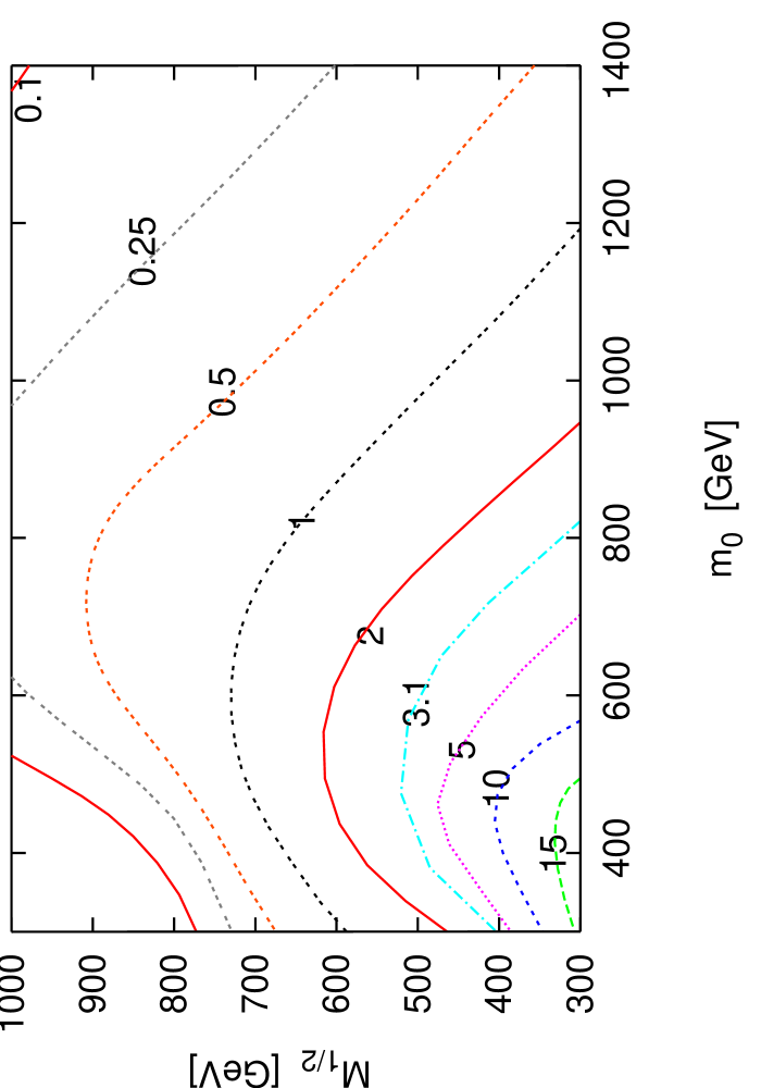
Figure 1: A contour plot of Br$(\tau\to\mu\gamma)\times 10^{7}$ in the $m_{0}-M_{1/2}$ plane with $\mu=120$ GeV and $A_{0}=0$. The present experimental bound is marked by the contour labelled ”3.1”.

Let us firstly look at the important lepton flavour violating decay $\ell_{i}\to\ell_{j}\gamma$. A contour plot showing the variation of the branching ratio for $\tau\to\mu\gamma$ in the $m_{0}-M_{1/2}$ plane is given in fig. 1. This plot shows that the rate for this process is very high over most of the plane and even in the low $m_{0}-M_{1/2}$ region the rate can exceed the present experimental upper bound. These large rates are a direct consequence of our choice of $Y_{\nu_{3}}^{\sf diag}\sim 1$.

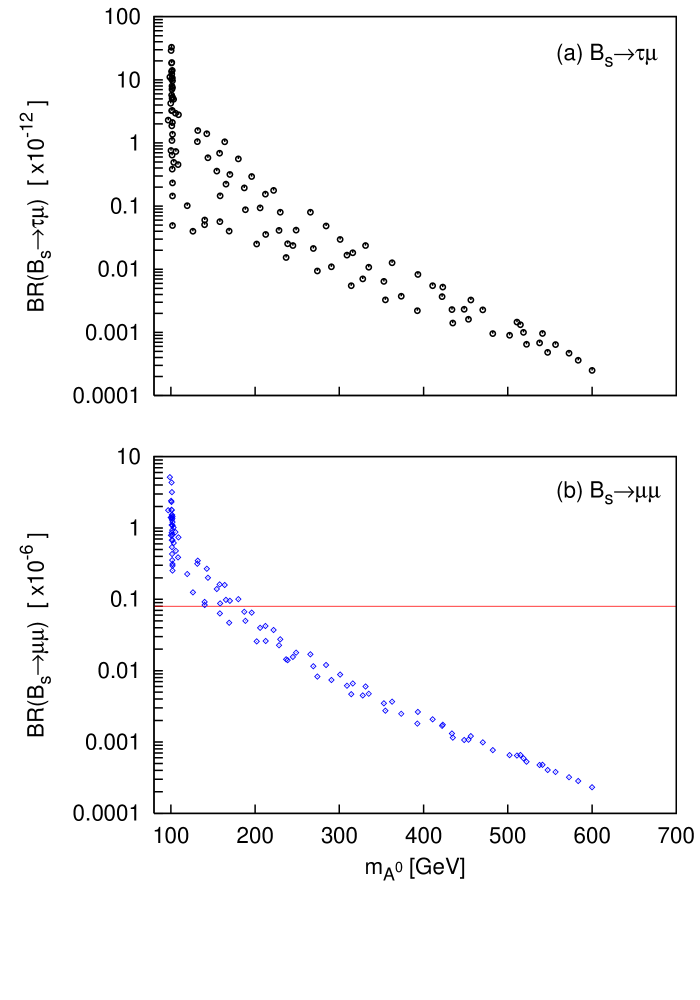
Figure 2: The Higgs mediated contribution to the branching ratio for $B_{s}\to\mu\mu(\tau\mu)$ is plotted in the lower(upper) panel against the Pseudoscalar Higgs mass, $m_{A^{0}}$. The horizontal line at $0.8\times 10^{-7}$ shows the present experimental upper bound.

The plot for the Higgs mediated contribution to the flavour changing neutral current decay, $B_{s}\to\mu^{+}\mu^{-}$, is presented in the lower panel of fig. 2. As previously reported, the branching ratio for $B_{s}\to\mu^{+}\mu^{-}$ is particularly interesting with rates ranging from $10^{-10}$ for heavy $m_{A^{0}}$ up to almost $10^{-5}$ for a particularly light $m_{A^{0}}$. The present $90\%$ C.L. experimental upper bound of $0.8\times 10^{-7}$[21] excludes the highest predicted rates and hence is beginning to probe the Higgs sector into the region $m_{A^{0}}\sim 150$ GeV. This rare decay is certainly of particular interest and future studies will continue to probe the Higgs sector to an even greater extent. Within the standard model the expectation is that Br$(B_{s}\to\mu^{+}\mu^{-})_{SM}\sim 10^{-9}$. Therefore we can see from fig. 2 that the Higgs mediated contribution to this process would dominate as long as $m_{A^{0}}<500$ GeV and this decay has the possibility of being the first indirect signal of supersymmetry.

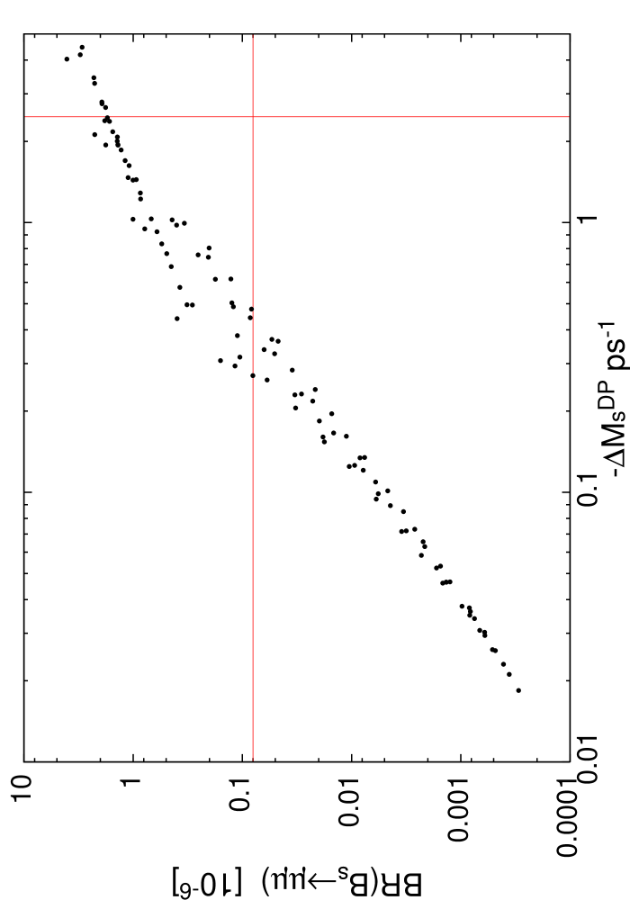
Figure 3: The correlation of Br$(B_{s}\to\mu^{+}\mu^{-})$ and $\Delta M_{s}^{\rm DP}$ are given for $f_{B_{s}}=230$ MeV (upper panel) and $f_{B_{s}}=259$ MeV(lower panel). The horizontal line in both panels shows the present experimental bound on Br$(B_{s}\to\mu^{+}\mu^{-})$. The vertical lines mark the central value of $(\Delta M_{s}^{\rm CDF}-\Delta M_{s}^{SM})$.

The lepton flavour violating decay $B_{s}\to\tau\mu$, plotted against the Pseudoscalar Higgs mass, is shown in the upper panel of fig. 2. This plot shows that the branching ratio for this decay could be as large as $\sim 10^{-10}$, but are certainly not as interesting as the flavour conserving decay just discussed. The branching ratio for the decay $\tau\to 3\mu$ are of a similar order of magnitude to those in the upper panel of fig. 2.

In the limit of large $\tan\beta$, $B_{s}\to\mu^{+}\mu^{-}$ and $\Delta M_{s}$ are correlated. This correlation is shown in the two panels of fig. 3. For these two panels the two different values of $f_{B_{s}}$ listed in eq. (14,15) are used. The upper panel ($f_{B_{s}}=230$ MeV) shows that the central value of $(\Delta M_{s}^{\rm CDF}-\Delta M_{s}^{\rm SM})$ coincides with the bound from Br$(B_{s}\to\mu^{+}\mu^{-})$. The lower panel ($f_{B_{s}}=259$ MeV) shows that the data points with $\Delta M_{s}^{\rm DP}$ at the central value, are in fact ruled out by the bound on Br$(B_{s}\to\mu^{+}\mu^{-})$. The uncertainty in the SM prediction for $\Delta M_{s}$ is rather large and in fact all of the data points of fig. 3 are allowed by the recent tevatron measurement. These two panels clearly show that the interpretation of the recent measurement depends crucially on the uncertainty in the determination of $f_{B_{s}}$.

The plot in fig. 4 shows the ratio, $\Delta M_{s}^{LL}/\Delta M_{s}^{LR}$, of the contributions to the operators $Q_{1}^{\rm SLL}$ and $Q_{2}^{\rm LR}$ as defined in eq. (3.1). It is commonly assumed that the contribution to the $Q_{2}^{\rm LR}$ operator, $\Delta M_{s}^{LR}$, is dominant. From fig. 4 we can see that the contribution of the $Q_{1}^{\rm SLL}$ operator, $\Delta M_{s}^{LL}$, is between 40% and 90% of $\Delta M_{s}^{LR}$ and hence is significant.

Our numerical results for the branching ratio of $H^{0}\to\tau\mu$ are presented in fig. 5c. The rates for this process are plotted against the Pseudoscalar higgs mass, $m_{A^{0}}$. The predicted rates range from $10^{-9}$ up to a few times $10^{-7}$. In fig. 5c we can see a broad band of points stretching from $m_{A^{0}}=100$ GeV up to $m_{A^{0}}=600$ GeV showing that most points are predicting a rate of around $10^{-8}$. The decay rate appears to be almost independent of the Pseudoscalar higgs mass, although there is a slight peak at the lower range of the higgs mass, which is where the highest rates are achieved. Notice that the data points shown in fig. 5 are divided into two groups. The grouping is determined by whether the $B_{s}\to\mu^{+}\mu^{-}$ bound is in excess or not, as indicated in the figure caption. From this grouping we can see that the points with the highest predicted $H^{0}\to\tau\mu$ rates appear to be excluded by the $B_{s}\to\mu^{+}\mu^{-}$ bound. In this way the Higgs mediated contribution to the $B_{s}$ decay can provide additional information on the allowed Higgs decay rate.

Figure 4: Plot for the ratio, $\Delta M_{s}^{LL}/\Delta M_{s}^{LR}$, of the Higgs contribution to the operators $Q_{1}^{SLL}$ and $Q_{2}^{LR}$.

Fig. 5b shows our predictions for the lepton flavour violating Pseudoscalar higgs decay, $A^{0}\to\tau\mu$. The rates for the decay of the Pseudoscalar are almost identical to those of the heavy CP-even higgs shown in fig. 5c.

The rate for the decay of the lightest higgs boson is shown in fig. 5a where it is again plotted against the Pseudoscalar higgs mass. The predicted rates for this decay show a very different dependence upon $m_{A^{0}}$, as they are spread over a large range from $10^{-11}$ to $10^{-7}$. The branching ratio for the lightest higgs appears to be inversely proportional to the Pseudoscalar higgs mass. Hence this LFV decay will only be interesting if $m_{A^{0}}<300$ GeV where its rate can be comparable to those for the other neutral higgs states. The data points for the lightest Higgs boson decay of fig. 5a have again been divided into two groups. As before, the two groupings depend upon whether the $B_{s}\to\mu^{+}\mu^{-}$ bound is being exceeded or not. The plot shows that the data points for particularly light Pseudoscalar Higgs mass are excluded by the $B_{s}\to\mu^{+}\mu^{-}$ bound. These excluded points correspond to the largest predictions for the decay $h^{0}\to\tau\mu$ and leaves, $3\times 10^{-9}$, the highest allow decay rate.

5 Conclusions

We have analysed a supersymmetric-seesaw model constrained by $SU(5)$ unification at the GUT scale. We have been concerned with making predictions for lepton flavour violating decay processes such as $\tau\to\mu\gamma$, $\mu\to e\gamma$ and $h^{0},\,H^{0},\,A^{0}\to\tau\mu$. With lepton flavour violation in mind, we chose to study the large $\tan\beta$ region of parameter space where such effects are enhanced. In addition we chose $Y_{\nu_{3}}^{\sf diag}\sim 1$ under the influence of $SO(10)$ unification in which $\tan\beta$ is naturally large.

Our numerical procedure utilises a complete top-down global $\chi^{2}$ fit to 24 low-energy observables. Through this electroweak fit we were able to analyse lepton flavour violating rates for rare charged lepton decays. The choice of a large third family neutrino Yukawa coupling naturally leads to large 23 lepton flavour violation. Within this scenario we have also used these numerical fits to analyse the FCNC processes $B_{s}\to\mu\mu(\tau\mu)$, $B_{s}^{0}\!-\!\bar{B}_{s}^{0}$ mixing and the lepton flavour violating decays of MSSM Higgs bosons. As a result, we have been about to make realistic predictions for this phenomenology while ensuring $\ell_{i}\to\ell_{j}\gamma$ and $b\to s\gamma$ constraints are satisfied.

Our model predicts a $\tau\to\mu\gamma$ rate near the present experimental limit. We have seen that the branching ratio for $H^{0}\to\tau\mu$ could be interesting with a rate as high as few $10^{-7}$. The Higgs mediated contribution to the branching ratio for $B_{s}\to\mu^{+}\mu^{-}$ was found to be particularly large and could even exceed the current experimental bound. In addition to the constraint of $\tau\to\mu\gamma$, we also saw that the $B_{s}\to\mu^{+}\mu^{-}$ bound may also act as a stringent restriction on the allowed rates for $\phi^{0}\to\tau\mu$. We found the rates for the LFV decays $B_{s}\to\tau\mu$ and $\tau\to 3\mu$ are rather small $<10^{-10}$.

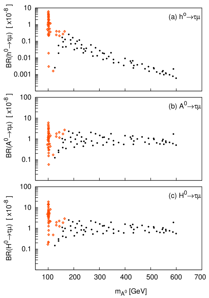
Figure 5: BR($H^{0}\to\tau\mu$) plotted against the Pseudoscalar Higgs mass, $m_{A^{0}}$. For each of these fitted points we have assumed the following values, $\mu=120$ GeV and $A_{0}=0$. Here the dots(circles) mark points for which $Br(B_{s}\to\mu^{+}\mu^{-})$ is below(above) the present experimental limit.

The correlation of $B_{s}\to\mu^{+}\mu^{-}$ and $\Delta M_{s}$ in the large $\tan\beta$ limit was also studied. The constraint from the recent tevatron measurement is highly dependant upon the determination of $f_{B_{s}}$. It was also found that the Higgs contribution to the operator $Q_{1}^{\rm SLL}$ can compete with that of the $Q_{2}^{\rm LR}$ operator.

References

- [1] J. K. Parry, arXiv:hep-ph/0510305.
- [2] C. S. Huang, W. Liao and Q. S. Yan, Phys. Rev. D 59, 011701 (1999) [arXiv:hep-ph/9803460]. S. R. Choudhury and N. Gaur, Phys. Lett. B 451 (1999) 86 [arXiv:hep-ph/9810307]. K. S. Babu and C. F. Kolda, Phys. Rev. Lett. 84, 228 (2000) [arXiv:hep-ph/9909476].
- [3] T. Blazek, S. F. King and J. K. Parry, Phys. Lett. B 589 (2004) 39 [arXiv:hep-ph/0308068].
- [4] J. Hisano and Y. Shimizu, Phys. Lett. B 565 (2003) 183 [arXiv:hep-ph/0303071]. N. Akama, Y. Kiyo, S. Komine and T. Moroi, Phys. Rev. D 64 (2001) 095012 [arXiv:hep-ph/0104263].
- [5] S. F. King and M. Oliveira, Phys. Rev. D 60 (1999) 035003 [arXiv:hep-ph/9804283].
- [6] T. Blažek and S. F. King, Phys. Lett. B 518 (2001) 109 [arXiv:hep-ph/0105005].
- [7] T. Blažek and S. F. King, arXiv:hep-ph/0211368.
- [8] F. Borzumati and A. Masiero, Phys. Rev. Lett. 57 (1986) 961. J. Hisano and D. Nomura, Phys. Rev. D 59 (1999) 116005 [arXiv:hep-ph/9810479]. J. R. Ellis, M. E. Gomez, G. K. Leontaris, S. Lola and D. V. Nanopoulos, Eur. Phys. J. C 14 (2000) 319 [arXiv:hep-ph/9911459]. S. Lavignac, I. Masina and C. A. Savoy, Phys. Lett. B 520 (2001) 269 [arXiv:hep-ph/0106245]. J. A. Casas and A. Ibarra, Nucl. Phys. B 618 (2001) 171 [arXiv:hep-ph/0103065]. T. Fukuyama, T. Kikuchi and N. Okada, Phys. Rev. D 68, 033012 (2003) [arXiv:hep-ph/0304190]. T. Fukuyama, A. Ilakovac and T. Kikuchi, arXiv:hep-ph/0506295.
- [9] R. Hempfling, Phys. Rev. D49, 6168 (1994). L. Hall, R. Rattazzi and U. Sarid, Phys. Rev. D50, 7048 (1994). M. Carena, M. Olechowski, S. Pokorski and C. Wagner, Nucl. Phys. B426, 269 (1994).
- [10] T. Blazek, S. Raby and S. Pokorski, Phys. Rev. D 52, 4151 (1995) [arXiv:hep-ph/9504364].
- [11] C. Hamzaoui, M. Pospelov and M. Toharia, Phys. Rev. D 59, 095005 (1999) [arXiv:hep-ph/9807350].
- [12] A. J. Buras, P. H. Chankowski, J. Rosiek and L. Slawianowska, Nucl. Phys. B 659 (2003) 3 [arXiv:hep-ph/0210145]. A. J. Buras, P. H. Chankowski, J. Rosiek and L. Slawianowska, Phys. Lett. B 546 (2002) 96 [arXiv:hep-ph/0207241].
- [13] S. Hashimoto, Int. J. Mod. Phys. A 20 (2005) 5133 [arXiv:hep-ph/0411126].
- [14] A. Gray et al. [HPQCD Collaboration], Phys. Rev. Lett. 95 (2005) 212001 [arXiv:hep-lat/0507015].
- [15] A. Abulencia [CDF - Run II Collaboration], arXiv:hep-ex/0606027.
- [16] V. M. Abazov et al. [D0 Collaboration], arXiv:hep-ex/0603029.
- [17] A. Dedes, J. R. Ellis and M. Raidal, Phys. Lett. B 549 (2002) 159 [arXiv:hep-ph/0209207]. D. Guetta, J. M. Mira and E. Nardi, Phys. Rev. D 59 (1999) 034019 [arXiv:hep-ph/9806359].
- [18] K. S. Babu and C. Kolda, Phys. Rev. Lett. 89 (2002) 241802 [arXiv:hep-ph/0206310].
- [19] E. Arganda, A. M. Curiel, M. J. Herrero and D. Temes, Phys. Rev. D 71 (2005) 035011 [arXiv:hep-ph/0407302]. A. Brignole and A. Rossi, Phys. Lett. B 566 (2003) 217 [arXiv:hep-ph/0304081]. A. Brignole and A. Rossi, Nucl. Phys. B 701 (2004) 3 [arXiv:hep-ph/0404211]. S. Kanemura, T. Ota and K. Tsumura, arXiv:hep-ph/0505191.
- [20] B. Aubert et al. [BABAR Collaboration], Phys. Rev. Lett. 92 (2004) 121801 [arXiv:hep-ex/0312027].
- [21] CDF collaboration, CDF Public Note 8176, www-cdf.fnal.gov