TUM-HEP-635/06

Reactor Neutrino Experiments with a
Large Liquid Scintillator Detector

Joachim Kopp,  Manfred Lindner,  Alexander Merle,
and Mark Rolinec

^,,, Physik–Department, Technische Universität München,

James–Franck–Strasse, 85748 Garching, Germany

^,, Max–Planck–Institut für Kernphysik,

Postfach 10 39 80, 69029 Heidelberg, Germany

We discuss several new ideas for reactor neutrino oscillation experiments with a Large Liquid Scintillator Detector. We consider two different scenarios for a measurement of the small mixing angle $\theta_{13}$ with a mobile $\bar{\nu}_{e}$ source: a nuclear-powered ship, such as a submarine or an icebreaker, and a land-based scenario with a mobile reactor. The former setup can achieve a sensitivity to $\sin^{2}2\theta_{13}\lesssim 0.004$ at the 90% confidence level, while the latter performs only slightly better than Double Chooz. Furthermore, we study the precision that can be achieved for the solar parameters, $\sin^{2}2\theta_{12}$ and $\Delta m_{21}^{2}$, with a mobile reactor and with a conventional power station. With the mobile reactor, a precision slightly better than from current global fit data is possible, while with a power reactor, the accuracy can be reduced to less than 1%. Such a precision is crucial for testing theoretical models, e.g. quark-lepton complementarity.

1 Introduction

Reactor experiments have always played a crucial role in neutrino physics. The first experimental evidence for the existence of the neutrino came from a reactor experiment [1, 2] and the most precise measurement of the oscillation parameter $\Delta m^{2}_{21}$ has been performed by the KamLAND experiment in Japan [3], where the $\bar{\nu}_{e}$-disappearance of neutrinos coming from the surrounding power plants at an average distance of approximately 180 km has been studied. KamLAND data has uniquely identified the large mixing angle scenario as the correct solution of the solar neutrino problem. Furthermore, the non-observation of reactor neutrino disappearance at baselines $\sim$ 1 km in the CHOOZ experiment in France is crucial for the current upper bound on the small mixing angle $\sin^{2}2\theta_{13}\lesssim 0.1$ [4]. The role of future reactor neutrino experiments in measuring or constraining the value of $\theta_{13}$ has already been extensively studied in the literature [5, 6, 7, 8]. Usually it is proposed to construct a relatively small detector close to a large nuclear power station. However, it is important to keep in mind that the performance of such a measurement besides the systematical uncertainties depends only on the total exposure, which is proportional to the product of the thermal power of the reactor, the detector mass, and the running time of the experiment. Thus, it is also imaginable to take advantage of a bigger multi-purpose detector, such as for example the Large Liquid Scintillator Detector LENA [9, 10], and combine it with a relatively small reactor. In this work, we consider using a mobile reactor, which will lead to interesting cancellations of systematical errors. Mobile reactors are widely used on nuclear-powered ships or submarines, but there are also ideas to construct land-based removable power stations that may be used to deliver electricity to very remote areas [11].

Apart from searching for nonzero $\theta_{13}$, an advanced reactor neutrino experiment can also provide a precision measurement of the solar oscillation parameters. It could improve the bounds on $\Delta m_{21}^{2}$, which are currently dominated by KamLAND, as well as those on the oscillation amplitude $\sin^{2}2\theta_{12}$, which are currently dominated by solar data. This improved precision is required, for example, to test quark-lepton complementarity [12] to a high precision, and to determine the neutrino mass hierarchy in $0\nu\beta\beta$-experiments [13, 14] and through the day-night effect in solar neutrino data [15]. A possible setup for such an advanced reactor neutrino experiment aiming at a precision measurement of the solar parameters has already been presented in [16]. We will complement the discussion given there by studying a setup involving a rather small, possibly mobile, nuclear reactor, and a LENA-like detector. Furthermore we will discuss the possibility of constructing such a large detector close to a nuclear power station. Since it is usually not desirable to construct a Large Liquid Scintillator Detector close to such a power plant since it would then be blind to Geo-neutrinos, supernova relic neutrinos, and other very faint sources, one would have to choose a reactor which is scheduled for permanent shutdown after several years of data taking, or a newly built power plant which only starts operation after the low-background measurements have been completed.

The outline of the paper is as follows: In Section 2, we will briefly review the neutrino oscillation framework and the underlying phenomenology of $\bar{\nu}_{e}$-disappearance measurements in reactor experiments. In Section 3, we will discuss the prospects of $\theta_{13}$ measurements with mobile reactors for two different scenarios, a nuclear-powered ship and a land-based mobile nuclear reactor. We will first describe the expectations from analytical estimates, and thereafter present results based on numerical calculations. We carefully include systematical uncertainties, which are the main limitation to the achievable sensitivity. Next, in Section 4, we will discuss precision measurements of the solar parameters $\sin^{2}2\theta_{12}$ and $\Delta m^{2}_{21}$ with both, a mobile reactor and a large nuclear power plant. Again, we will give analytical estimates as well as numerical results. The latter will include a careful treatment of the Geo-neutrino background which turns out to have a significant impact on the optimization of the baseline.

2 The neutrino oscillation framework

The relevant oscillation channel for a reactor neutrino experiment is $\bar{\nu}_{e}\rightarrow\bar{\nu}_{e}$ disappearance. The corresponding exact formula for the vacuum survival probability of an electron anti-neutrino $\bar{\nu}_{e}$ with energy $E$ at a baseline $L$ is given by [17]:

$$P(\bar{\nu}_{e}\rightarrow\bar{\nu}_{e})=1-\sin^{2}2\theta_{13}\sin^{2}\Delta_{31}-(\cos^{4}\theta_{13}\sin^{2}2\theta_{12}+\sin^{2}\theta_{12}\sin^{2}2\theta_{13})\sin^{2}\Delta_{21}+\\ +\sin^{2}\theta_{12}\sin^{2}2\theta_{13}(\frac{1}{2}\sin 2\Delta_{21}\sin 2\Delta_{31}+2\sin^{2}\Delta_{31}\sin^{2}\Delta_{21}),$$ (1)

where $\Delta_{21}\equiv\Delta m_{21}^{2}L/(4E)$ and $\Delta_{31}\equiv\Delta m_{31}^{2}L/(4E)$. The parameters involved are the “reactor angle” $\theta_{13}$, the “atmospheric mass squared difference” $\Delta m_{31}^{2}$, and the “solar parameters” $\theta_{12}$ and $\Delta m_{21}^{2}$. The solar parameters have been measured by the SNO and KamLAND experiments [18, 19, 20, 3, 21], and due to the observed MSW effect [22, 23], the sign of $\Delta m_{21}^{2}$ is also known. The atmospheric parameters have been measured by Super-Kamiokande [24, 25], K2K [26, 27], and MINOS [28, 29], but the sign of $\Delta m_{31}^{2}$ has not been determined yet. Considering the small mixing angle $\theta_{13}$, there exists only an upper bound which is dominated by the CHOOZ experiment [4]. The best-fit values and allowed intervals for all oscillation parameters from a global three-flavor analysis can be found in [30, 31, 32, 33].

While our numerical simulations are based on the full three-flavor treatment, we will only use zeroth-order approximations for the analytical estimates. These approximations are given by

$$P_{\mathrm{sol}}(\bar{\nu}_{e}\rightarrow\bar{\nu}_{e})\approx 1-\sin^{2}2\theta_{12}\sin^{2}\Delta_{21},$$ (2)

for the measurement of the solar parameters, and by

$$P_{\mathrm{atm}}(\bar{\nu}_{e}\rightarrow\bar{\nu}_{e})\approx 1-\sin^{2}2\theta_{13}\sin^{2}\Delta_{31}$$ (3)

for the (13)-oscillations and are justified by the numerical values of the parameters. Since $|\Delta m_{31}^{2}|\gg\Delta m_{21}^{2}$, the (13)-oscillation length is much smaller than the (12)-oscillation length, so a typical $\theta_{13}$ experiment located at the first atmospheric oscillation maximum is hardly affected by the solar terms. On the other hand, for the amplitudes it holds that $\sin^{2}2\theta_{12}\gg\sin^{2}2\theta_{13}$, so the (13)-oscillation constitutes a negligible perturbation in a measurement of $\theta_{12}$ and $\Delta m_{21}^{2}$.

For the oscillation parameters, we assume the following true values in the numerical simulations:

$$\begin{array}[]{rclrcl}\Delta m_{31}^{2}&=&2.5\cdot 10^{-3}\textrm{eV}^{2},&\hskip 56.9055pt\sin^{2}2\theta_{23}&=&1,\\ \Delta m_{21}^{2}&=&8.2\cdot 10^{-5}\textrm{eV}^{2},&\hskip 56.9055pt\sin^{2}2\theta_{12}&=&0.83.\end{array}$$ (4)

3 $\boldsymbol{\theta_{13}}$ measurement with a mobile reactor

In this section we consider the potential of a mobile electron anti-neutrino source, combined with a Large Liquid Scintillator Detector, to measure the small mixing angle $\theta_{13}$. We assume that the reactor is placed at two different baselines, the “near” and “far” positions, consecutively. The major limitation for such an experiment will be the systematical errors. If these are not under control, any deficit in the observed neutrino flux could be attributed either to neutrino oscillations or to a systematical bias in the initial reactor neutrino flux or in the detector properties. We will consider two scenarios with different systematical uncertainties:

• A nuclear-powered ship, e.g. a submarine or an icebreaker (cf. [34]):
  Since the reactor is not required to be shut down in order to change its position, and since it can be moved between the near and far positions frequently, it is reasonable to assume that the unoscillated neutrino flux and spectrum are the same at both positions. This will turn out to be crucial for the cancellation of the associated systematical errors. Such a nuclear-ship scenario could only be realized, if the detector were located under water, e.g. in the Mediterranean Sea.

• A land-based nuclear reactor, such as the SSTAR design [11]:
  Here, the reactor needs to be shut down in order to be maneuverable, and such a movement will only be done once, so the neutrino flux and spectrum at the near and far positions will be uncorrelated. This problem could be alleviated by using a small dedicated near detector to reduce the uncertainties to those associated with the near detector, which are typically smaller than those associated with the reactor.

For both scenarios, we consider a detector with a fiducial mass of 45 kt, which corresponds to the proposed LENA detector [9, 10]. Note that some of our conclusions can also be applied to reactor neutrino experiments in which not the source, but the detector is mobile [35]. In such a scenario, the detector will only be moved once, so it is similar to our land-based scenario. However, the detailed impact of the systematical errors is different: If the reactor is movable, only the neutrino flux and spectrum uncertainties will be uncorrelated in the two phases of the experiment, while for a movable detector scenario, also at least some of the detector-related uncertainties should remain uncorrelated. Apart from this, the feasibility is different since mobile nuclear reactors do already exist and their development is continuing, while there is no practical experience on mobile neutrino detectors yet. Note, that only for the nuclear-powered ship scenario it can be assumed that all neutrino flux and spectrum associated systematical uncertainties are completely correlated in the two phases of the experiment, since, as mentioned above, a frequent change between the near and far position is possible.

To study the sensitivity of reactor neutrino experiments, we use a $\chi^{2}$ analysis, incorporating pull terms for the proper treatment of systematical uncertainties. In our numerical calculations we assume the events to follow a Poisson distribution, but for illustrative purposes it is sufficient to consider the Gaussian approximation, which is very good due to the large event rates in a $\theta_{13}$ reactor experiment. For the nuclear-powered ship scenario, our $\chi^{2}$ expression has the form

$$\chi^{2}=\sum_{A=N,F}\sum_{i}\frac{1}{N_{i}^{A}}\big{[}T_{i}^{A}(a_{\rm norm},a_{\rm det},a_{\mathrm{shape},i},a_{\rm bkg},b)-N_{i}^{A}\big{]}^{2}+\\ +\frac{a_{\rm norm}^{2}}{\sigma_{\rm norm}^{2}}+\frac{a_{\rm det}^{2}}{\sigma_{\rm det}^{2}}+\sum_{i}\frac{a_{\mathrm{shape},i}^{2}}{\sigma_{\rm shape}^{2}}+\frac{a_{\rm bkg}^{2}}{\sigma_{\rm bkg}^{2}}+\frac{b^{2}}{\sigma_{b}^{2}}.\hskip 56.9055pt$$ (5)

Here, $N_{i}^{N}$ and $N_{i}^{F}$ denote the event numbers in the $i$-th bin at the near and far positions, respectively. These event rates are calculated with the values for the oscillation parameters given in Eq. (4). Correspondingly, $T_{i}^{A}$ are the theoretically predicted event rates for certain fit values of the oscillation parameters, and for the systematical biases $a_{j}$ and $b$. The second line of Eq. (5) contains the pull terms which represent prior knowledge about the systematics parameters. They give a penalty to biases that are much larger than the estimated systematical errors. In detail, we introduce the following systematical error sources:

• The flux normalization uncertainty $\sigma_{\rm norm}=2.0\%$, which is correlated between the near and far positions in the nuclear-powered ship scenario, but not in the land-based scenario. It accounts for the limited accuracy with which the thermal reactor power and thus the emitted neutrino flux can be determined.

• The detector normalization error $\sigma_{\rm det}=2.0\%$, which describes uncertainties associated with the fiducial detector mass, the cross sections, the scintillator properties, and the analysis cuts.

• A background flux error $\sigma_{\rm bkg}=10.0\%$. As backgrounds, we take into account Geo-neutrinos, amounting to about 1450 events per year [36, 37, 38], and a diffuse reactor background of about 850 events per year, which corresponds to the estimated flux from the 20 closest reactors at the proposed LENA site in Pyhäsalmi (Finland) [39, 40]. By taking into account all nuclear reactors in the world, the background rate would only increase marginally.

• The shape uncertainty, $\sigma_{\rm shape}=2.0\%$, which describes the limited knowledge of the reactor neutrino spectrum. The corresponding parameter $a_{\mathrm{shape},i}$ is independent for each bin $i$, hence the index $i$ is introduced. This parameterization follows the discussion in [6].

• An energy calibration error $\sigma_{b}=2.0\%$, which is parameterized by $b$.

These errors are summarized in Table 1. The dependence of the $T_{i}^{A}$ on the systematical biases is given by

Reactor Neutrino Flux	2.0%
Detector Normalization	2.0%
Detector Energy Calibration	2.0%
Shape Error	2.0% per bin
Normalization of 1% background	10.0%

Table 1: The systematical uncertainties that are assumed in our numerical simulations (based on [8, 41]).

$$T_{i}^{A}=(1+a_{\rm norm}+a_{\rm det}+a_{\mathrm{shape},i})\tilde{S}_{i}^{A}(b)+(1+a_{\rm bkg}+a_{\rm det})\tilde{B}_{i}^{A}(b),$$ (6)

where in turn $\tilde{S}_{i}^{A}(b)$ nd $\tilde{B}_{i}^{A}(b)$ are the signal and background rates for the wrong energy binning implied by nonzero $b$. They are obtained from the correctly binned rates $S_{i}^{A}$ and $B_{i}^{A}$ according to

$$\tilde{S}_{i}^{A}(b) =(1+b)[(S_{{\lfloor\delta\rfloor}+1}-S_{\lfloor\delta\rfloor})(\delta-{\lfloor\delta\rfloor})+S_{\lfloor\delta\rfloor}],$$ (7)

$$\delta =b\cdot(i+t_{0}+\tfrac{1}{2})+i,$$ (8)

and a similar expression for $\tilde{B}_{i}^{A}$ (see also ref. [6]). The quantity $t_{0}$ in Eq. (8) is the energy threshold of the detector, expressed in units of the bin width. We have used the Gauss bracket ${\lfloor\cdot\rfloor}$ to denote the floor function. The expression in square brackets in Eq. (7) is essentially a linear interpolation between the events in bin ${\lfloor\delta\rfloor}$ and those in bin ${\lfloor\delta\rfloor}+1$. If $b$ is not too large, the energy calibration never changes by more than the bin width, so that ${\lfloor\delta\rfloor}=i$. The factor $(1+b)$ in front accounts for the change of the bin width implied by $b$.

The $\chi^{2}$ expression for the land-based scenario is similar to Eq. (5), but since the reactor flux and spectrum are uncorrelated between the near and far positions in this scenario, $a_{\rm norm}$ and $a_{\mathrm{shape},i}$ get an additional index $A=N,F$.

3.1 Analytical estimates

We will now show that, for the nuclear-powered ship scenario, the most important systematical errors can be eliminated in the actual measurement of $\theta_{13}$ if the reactor is positioned at two different baselines consecutively. To quantify the performance of the experiment, we consider the sensitivity to $\sin^{2}2\theta_{13}$, which is defined as the limit that can be set on $\sin^{2}2\theta_{13}$ assuming that the true value is 0. This quantity can be calculated by comparing the simulated event rates for non-zero test values of $\sin^{2}2\theta_{13}$ with those for $\sin^{2}2\theta_{13}=0$ in a $\chi^{2}$ analysis.

For an analytical estimate, we consider a simplified version of Eq. (5), keeping only the reactor flux error $\sigma_{\rm norm}$ and the detector normalization error $\sigma_{\rm det}$, but neglecting spectral uncertainties, energy calibration errors, and backgrounds:

$$\chi^{2}=\sum_{A=N,F}\sum_{i=1}^{n}\frac{1}{N_{i}^{A}}\left[N_{i}^{A}(1+a_{\rm norm}+a_{\rm det})(1-\sin^{2}2\theta_{13}\sin^{2}\Delta_{i}^{A})-N_{i}^{A}\right]^{2}+\frac{a_{\rm norm}^{2}}{\sigma_{\rm norm}^{2}}+\frac{a_{\rm det}^{2}}{\sigma_{\rm det}^{2}}.$$ (9)

Here, the index $i$ runs over all $n$ energy bins, while $A$ takes the values $N$ and $F$ for the near and far baselines, respectively. $N_{i}^{A}$ is the total event rate in the $i$-th bin at baseline $L^{A}$ without oscillations, and $\Delta_{i}^{A}=\Delta m_{31}^{2}L^{A}/4E_{i}$ is the oscillation phase for baseline $L^{A}$ and energy $E_{i}$.

Since the systematical biases $a_{\rm norm}$ and $a_{\rm det}$ as well as the oscillation amplitude $\sin^{2}2\theta_{13}$ are small, Eq. (9) can be approximated by

$$\chi^{2}=\sum_{A=N,F}\sum_{i=1}^{n}N_{i}^{A}\left(a_{\rm norm}+a_{\rm det}-\sin^{2}2\theta_{13}\sin^{2}\Delta_{i}^{A}\right)^{2}+\frac{a_{\rm norm}^{2}}{\sigma_{\rm norm}^{2}}+\frac{a_{\rm det}^{2}}{\sigma_{\rm det}^{2}}.$$ (10)

$a_{\rm norm}$ and $a_{\rm det}$ are fitted by minimizing $\chi^{2}$, therefore we calculate

$$\frac{\partial\chi^{2}}{\partial a_{\rm norm}} =\sum_{A=N,F}\sum_{i=1}^{n}2N_{i}^{A}\left(a_{\rm norm}+a_{\rm det}-\sin^{2}2\theta_{13}\sin^{2}\Delta_{i}^{A}\right)+\frac{2a_{\rm norm}}{\sigma_{\rm norm}^{2}},$$ (11)

$$\frac{\partial\chi^{2}}{\partial a_{\rm det}} =\sum_{A=N,F}\sum_{i=1}^{n}2N_{i}^{A}\left(a_{\rm norm}+a_{\rm det}-\sin^{2}2\theta_{13}\sin^{2}\Delta_{i}^{A}\right)+\frac{2a_{\rm det}}{\sigma_{\rm det}^{2}}.$$ (12)

By requiring the expressions (11) and (12) to be zero and taking their difference, we obtain

$$a_{\rm norm}=\frac{\sigma_{\rm norm}^{2}}{\sigma_{\rm det}^{2}}a_{\rm det}.$$ (13)

Substituting this back into Eq. (11) or (12), and assuming the $N_{i}^{A}$ to be very large, the systematical biases can be expressed as

$$a_{\rm det} =\frac{\sin^{2}2\theta_{13}}{1+\sigma_{\rm norm}^{2}/\sigma_{\rm det}^{2}}\cdot\frac{\sum_{A=N,F}\sum_{i=1}^{n}N_{i}^{A}\sin^{2}\Delta_{i}^{A}}{\sum_{A=N,F}\sum_{i=1}^{n}N_{i}^{A}},$$ (14)

$$a_{\rm norm} =\frac{\sin^{2}2\theta_{13}}{1+\sigma_{\rm det}^{2}/\sigma_{\rm norm}^{2}}\cdot\frac{\sum_{A=N,F}\sum_{i=1}^{n}N_{i}^{A}\sin^{2}\Delta_{i}^{A}}{\sum_{A=N,F}\sum_{i=1}^{n}N_{i}^{A}}.$$ (15)

Thus, in the limit $N_{i}^{A}\rightarrow\infty$, $\chi^{2}$ is approximately given by

$$\chi^{2}=\sin^{4}2\theta_{13}\sum_{A=N,F}\sum_{i=1}^{n}N_{i}^{A}\left(\frac{\sum_{B=N,F}\sum_{j=1}^{n}N_{j}^{B}\sin^{2}\Delta_{j}^{B}}{\sum_{B=N,F}\sum_{j=1}^{n}N_{j}^{B}}-\sin^{2}\Delta_{i}^{A}\right)^{2}.$$ (16)

The $1\sigma$ sensitivity limit for $\sin^{2}2\theta_{13}$ is determined by the condition $\chi^{2}=1$:

$$\sigma(\sin^{2}2\theta_{13})=\left[\sum_{A=N,F}\sum_{i=1}^{n}N_{i}^{A}\left(\frac{\sum_{B=N,F}\sum_{j=1}^{n}N_{j}^{B}[\sin^{2}\Delta_{j}^{B}-\sin^{2}\Delta_{i}^{A}]}{\sum_{B=N,F}\sum_{j=1}^{n}N_{j}^{B}}\right)^{2}\right]^{-1/2}\ \stackrel{{\scriptstyle N_{i}^{A}\rightarrow\infty}}{{\longrightarrow}}\ 0.$$ (17)

This means that the sensitivity will be good if $N_{i}^{A}$ is large and $|\sin^{2}\Delta_{j}^{B}-\sin^{2}\Delta_{i}^{A}|$ is not too close to zero. Therefore an optimal experiment involves one measurement very close to the reactor ($\sin^{2}\Delta_{i}^{A}\approx 0$) and one around the first oscillation maximum ($\sin^{2}\Delta_{i}^{A}\approx 1$).

Now compare this to the case where the reactor position is fixed, i.e. $L^{N}=L^{F}$. Then, $N_{i}^{N}=N_{i}^{F}=N_{i}/2$ and $\sin^{2}\Delta_{i}^{N}$ = $\sin^{2}\Delta_{i}^{F}$ = $\sin^{2}\Delta_{i}$. If we perform only a total rate analysis ($n=1$), the right hand side of Eq. (16) will be very close to zero. This means that we have to consider the next-order term:

$$\chi^{2}=\frac{a_{\rm norm}^{2}}{\sigma_{\rm norm}^{2}}+\frac{a_{\rm det}^{2}}{\sigma_{\rm det}^{2}}=\sin^{4}2\theta_{13}\left(\frac{\sum_{i}N_{i}\sin^{2}\Delta_{i}}{\sum_{i}N_{i}}\right)^{2}\frac{1}{\sigma_{\rm det}^{2}+\sigma_{\rm norm}^{2}}.$$ (18)

In this case, $\sigma(\sin^{2}2\theta_{13})$ is of order $\sqrt{\sigma_{\rm det}^{2}+\sigma_{\rm norm}^{2}}$.

In reality, $n$ will be chosen greater than $1$ in order to exploit spectral information. In this case, the right hand side of Eq. (16) can be interpreted as a comparison of the oscillation phase in bin $i$, $\sin^{2}\Delta_{i}^{A}$, to the average oscillation phase $\sum_{B}\sum_{j}N_{j}^{B}\sin^{2}\Delta_{j}^{B}/\sum_{B}\sum_{j}N_{j}^{B}$. Therefore, this term is sensitive to the spectral distortion caused by neutrino oscillations, and in principle, the systematical errors $\sigma_{\rm norm}$ and $\sigma_{\rm det}$ can be eliminated without going to different baselines. This seems reasonable because the $L/E$ dependence of the oscillation probability Eq. (3) implies that measuring at different energies is equivalent to measuring at different baselines. However, our numerical results presented below will show, that in reality it is still highly advantageous to change the baseline.

3.2 Numerical results

To demonstrate the full impact of systematical errors on the $\sin^{2}2\theta_{13}$ sensitivity, we have performed numerical simulations with a modified version of the GLoBES software [42], which incorporates a $\chi^{2}$ expression similar to Eq. (5), but is based on the more realistic assumption of Poisson statistics and uses the exact three-flavor oscillation probability without applying any approximations. The reactor spectrum has been taken from [43, 3], and the cross sections are from [44]. We assume an energy resolution of $0.091\sqrt{E/\textrm{MeV}}$ MeV ([10, 45]) and sort the events into 67 energy bins. Additionally, we assume that the reactor is located at baseline $L_{1}$ for $t_{\textrm{tot}}L_{1}^{2}/(L_{1}^{2}+L_{2}^{2})$ and at baseline $L_{2}$ for $t_{\textrm{tot}}L_{2}^{2}/(L_{1}^{2}+L_{2}^{2})$, where $t_{\textrm{tot}}$ is the total running time of the experiment. This ensures that the numbers of events in the near and far detectors are comparable. We take $L_{1}=0.1$ km and $L_{2}=1.3$ km.

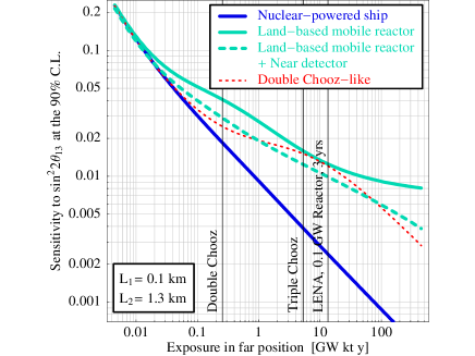
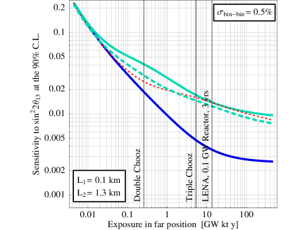
Figure 1: Sensitivity to $\sin^{2}2\theta_{13}$ at the 90% confidence level as a function of the exposure for a nuclear-powered ship scenario (solid blue/black curve), a land-based mobile reactor scenario (solid cyan/grey curve), a land-based mobile reactor scenario with an associated near detector (dashed cyan/grey curve), and a Double Chooz-like setup (dotted red/black curve) with one reactor and near and far detectors. The left plot has been calculated under the assumption of no bin-to-bin errors, while the right one includes an uncertainty $\sigma_{\rm bin-bin}=0.5\%$.

Figure 1 shows the sensitivity of different scenarios as a function of the total exposure $\Phi$. In addition to the nuclear-powered ship and land-based scenarios that where discussed above, we also show for comparison the performance of a setup similar to Double Chooz [8] with one reactor and two detectors. In this Double Chooz-like scenario, the uncorrelated detector normalization and energy calibration errors are taken to be only 0.6% and 0.5% because many detector-side effects will cancel. For very low exposures, $\Phi\leq 0.02$ GW kt y, all three scenarios are limited by the overall statistics and by backgrounds. As long as bin-to-bin errors, that are uncorrelated between the different bins as $\sigma_{\rm shape}$ and additionally uncorrelated between the near and far phase, are neglected (see left plot in Fig. 1), the nuclear-powered ship scenario (solid blue/black curve) follows the statistical limit also for larger exposures because systematical errors cancel completely in this scenario, as expected from our analytical estimates. For the land-based scenario (solid cyan/gray curve), only the systematical errors associated with the detector cancel because we have assumed the reactor neutrino flux to be completely uncorrelated before and after the displacement of the reactor. For the spectrum, we assume a partial correlation, which is parameterized by introducing in addition to the shape error from Eq. (5) a new bin-dependent bias with a 1% error, which is only present at baseline $L_{2}$. As soon as the exposure exceeds 0.02 GW kt y, the sensitivity of the land-based scenario becomes limited by the uncorrelated flux normalization error. As the exposure increases further, this error becomes less dominant because the event numbers are so large that spectral information can be exploited. However, above 10 GW kt y, the uncorrelated shape error prevents a further increase in the sensitivity. This can be avoided if a small near detector with a mass of 45 t, an uncorrelated normalization error of 0.6%, and an uncorrelated energy calibration error of 0.5% is employed (dashed cyan/gray curve). Finally, in the Double Chooz-like scenario (dotted red/black curve), the errors associated with the reactor cancel, but those associated with the detectors remain. As the reactor flux has larger uncertainties than the detector normalization, this scenario is better than the land-based mobile reactor scenario for luminosities of 0.02 GW kt y – 6 GW kt y. At the onset of the spectrally dominated regime, the two curves meet again, but for very large luminosities the Double Chooz-like near/far scenario is again better than the land-based scenario (without associated near detector) because the shape error is canceled by the near detector.

The vertical lines in Figure 1 indicate the total exposures that are to be expected from the Double Chooz experiment, its possible upgrade scenario Triple Chooz (see [41]), and a possible total exposure of the mobile scenarios (0.1 GW thermal power of the mobile reactor source, 3 years data taking, 45 kt fiducial mass of the LENA detector). While the performance of the land-based mobile reactor scenario is comparable to the Double Chooz-like scenario (dotted red/black curve) taken at the same total exposure, a nuclear-powered ship scenario could, due to the excellent cancellation of systematical uncertainties, achieve a sensitivity limit $\sin^{2}2\theta_{13}\lesssim 0.003$ at the 90% confidence level.

Even under the assumption of an uncorrelated bin-to-bin error $\sigma_{\rm bin-bin}=0.5\%$ (see right hand plot of Fig 1), this excellent sensitivity decreases only marginally. $\sigma_{\rm bin-bin}$ parameterizes all kinds of unknown backgrounds and detector non-linearities. It is introduced in Eq. (5) in a similar way as $\sigma_{\rm shape}$, but the corresponding parameter $a_{{\rm bin-bin},i}^{A}$ depends not only on the bin, but also on the detector position, hence the index $A=N,F$ for near and far phase is introduced.

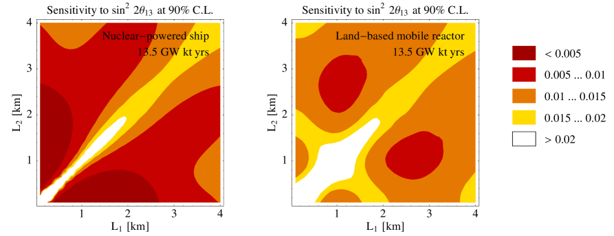
Figure 2: Sensitivity limit to $\sin^{2}2\theta_{13}$ at the 90% confidence level for the nuclear-powered ship scenario (left) and the land-based scenario (right) as function of the near and far baselines.

Let us now address the issue of choosing the optimal baselines for the two phases of the experiment. Figure 2 shows that, for the nuclear-powered ship scenario, it is clearly advantageous to choose $L_{1}$ very close to the reactor in order to measure the unoscillated flux (0th oscillation minimum), and $L_{2}$ around the first oscillation maximum at about 1.3 km. For the land-based scenario, the overall sensitivity is worse, but now the baseline combination 1st minimum/1st maximum gives better results than the combination 0th minimum/1st maximum. From a practical point of view, this turns out to be advantageous because in the land-based scenario it will usually not be possible to move the reactor close to the detector, as the latter will be located deep underground. We have also studied scenarios in which more than two different baselines are used. However, no significant improvement in the sensitivity could be achieved this way.

4 Measurement of the solar parameters

An often neglected topic is the issue of a precise measurement of the so-called solar oscillation parameters ($\theta_{12}$ and $\Delta m_{21}^{2}$) with a reactor neutrino experiment located at the first solar oscillation maximum (earlier studies can be found in [16, 46, 47]). Although e.g. the value of $\theta_{12}$ has been determined by solar experiments and KamLAND [33] to be about $33^{\circ}\pm 3^{\circ}$, which seems to be quite accurate, it should be stressed that the relative uncertainty is still about 10%. Since precise knowledge of $\theta_{12}$ is very important, in particular for the distinction between the normal and inverted neutrino mass hierarchy in $0\nu\beta\beta$-experiments [13, 14] and via the day-night effect of solar neutrinos [15], as well as for exploring the possible existence of quark-lepton complementarity [12], a more precise measurement is desirable, and we will show that it can be performed with a Large Liquid Scintillator Detector.

For the measurement of the solar oscillation parameters, two different scenarios are considered: the first one (“SMALL”) employs a mobile reactor with a thermal power of 0.5 GW_th, with 2 years of data taking, and the second one (“LARGE”) is a power reactor (10 GW_th, 5 years data taking) located at a suitable distance from the detector. It is desirable that this reactor should not be running during the whole lifetime of the detector, so that the latter can also pursue physics goals which require low backgrounds, e.g. the search for Geo-neutrinos, supernova relic neutrinos, and proton decay. Of course, no one would build a detector like LENA voluntarily in the direct neighborhood of such a power station, since the neutrino flux coming from this reactor would dominate all events from other neutrino sources and the detector would be effectively unusable for experiments other than long baseline oscillation measurements. However, if the reactor is scheduled to be shut down after the first years of data taking with the Large Liquid Scintillator Detector or if it is just planned to be built but there is enough time left to take data for the other measurements with the detector, this will not cause any problems.

The detector properties and systematical errors are the same as in Section 3, but since background sources, in particular Geo-neutrinos, are much more important now, they need to be treated in a more sophisticated way.

In Refs. [16, 46] it has been shown, that Geo-neutrinos have a strong influence in a “large reactor – small detector setup”, namely SADO. Since we analyze a much larger detector, this influence could be stronger here, even if the “product” of the reactor and the detector size (i.e. the total exposure) is similar. However, as will be shown, our results are still comparable to those obtained by the previous analyses.

The $\chi^{2}$ function for Section 4, including contributions from Geo–neutrinos in a more accurate way, has the following form:

$$\chi^{2}=\sum_{i}\frac{1}{N_{i}}\big{[}T_{i}(a_{\rm norm},a_{\rm det},a_{\rm reac},a_{\rm U},a_{\rm Th},b)-N_{i}\big{]}^{2}+\\ +\frac{a_{\rm norm}^{2}}{\sigma_{\rm norm}^{2}}+\frac{a_{\rm det}^{2}}{\sigma_{\rm det}^{2}}+\frac{a_{\rm reac}^{2}}{\sigma_{\rm reac}^{2}}+\frac{a_{\rm U}^{2}}{\sigma_{\rm U}^{2}}+\frac{a_{\rm Th}^{2}}{\sigma_{\rm Th}^{2}}+\frac{b^{2}}{\sigma_{b}^{2}}.\hskip 56.9055pt$$ (19)

The meaning of the parameters is the same as in Sec. 3, but the background errors $\sigma_{\rm bkg}$ are now split up into the contributions coming from distant nuclear reactors ($\sigma_{\rm reac}$), the Geo-neutrinos from the uranium decay chain ($\sigma_{\rm U}$), and the Geo-neutrinos from the thorium decay chain ($\sigma_{\rm Th}$).

We will consider three different situations to show the impact of the Geo-neutrino background:

• No Geo-neutrinos: In this case, Geo-neutrinos are completely absent, and only the background from distant nuclear reactors is taken into account. As in Sec. 3, it yields 850 events per year. The uncertainty in the flux normalization is taken to be 2%.

• Geo-neutrinos with a 10% uncertainty: Here, Geo-neutrinos are taken into account, and the uncertainty in their flux is assumed to be 10%. We use independent normalization factors for neutrinos originating from the uranium decay chain and those originating from the thorium decay chain (cf. Eq. (19)) because the relative abundances of these elements in the Earth depend strongly on the geological model [48]. However, as central value, we assume the ratio of the thorium and uranium abundances to be 3.9, as given in [48]. The decay chains of other long-lived radioactive isotopes, e.g. K-40, are not relevant for our discussion because they yield anti-neutrino energies below the detection threshold of 1.8 MeV. The Geo-neutrino spectra in our simulations are taken from [38, 37]. The reactor background is the same as in the scenario without Geo-neutrinos.

• Geo-neutrinos with a 100% uncertainty: This scenario is equivalent to the previous one, but now the uncertainties in the two Geo-neutrino contributions are taken to be 100%.

4.1 Analytical estimates

The optimum baseline for a measurement of $\theta_{12}$ can be estimated analytically if we neglect backgrounds and systematical errors for simplicity, and perform a total rates analysis, neglecting spectral information. Again, we start with the $\chi^{2}$-function for this scenario:

$$\chi^{2}=\frac{\left[N\left(1-\sin^{2}2\bar{\theta}_{12}\sin^{2}\bar{\Delta}\right)-N\left(1-\sin^{2}2\theta_{12}\sin^{2}\Delta\right)\right]^{2}}{N\left(1-\sin^{2}2\theta_{12}\sin^{2}\Delta\right)}.$$ (20)

Here, the barred values are the theoretical predictions, calculated with fit-values for the parameters, and the ones without bars come from the observed event rates, calculated with the assumed true parameter values from Eq. (4). The $\Delta$’s are defined as $\Delta\equiv\Delta m_{21}^{2}L/(4E)$ and $\bar{\Delta}\equiv\overline{\Delta m^{2}_{21}}L/(4E)$, where $L$ denotes the baseline and $E$ the energy of the incoming neutrino. For convenience, we additionally introduce the abbreviations $s\equiv\sin 2\theta_{12}$ and $\bar{s}\equiv\sin 2\bar{\theta}_{12}$, and write the unoscillated event rate as $N=N_{0}/L^{2}$, where $N_{0}$ is independent of $L$. Furthermore, for the analytical estimate of the optimal baseline for a measurement of the solar mixing angle, we neglect parameter correlations between the solar parameters and assume a fixed $\Delta m_{21}^{2}=\overline{\Delta m^{2}_{21}}$. Now, the $\chi^{2}$-function becomes:

$$\chi^{2}=\frac{N_{0}\sin^{4}\Delta}{L^{2}\left(1-s^{2}\sin^{2}\Delta\right)}\left(s^{2}-\bar{s}^{2}\right)^{2}.$$ (21)

Since we want to measure the amplitude $\sin^{2}2\theta_{12}$ of the oscillations, we can already guess that the optimum baseline should correspond to an oscillation phase of approximately $\pi/2$, because there, the oscillation has a maximum, and $\pi/2$ is the closest point to the detector with this property. With a simple Taylor expansion, one then gets:

$$\sin\Delta=\sin\left(\frac{\pi}{2}+\left(\Delta-\frac{\pi}{2}\right)\right)\approx 1-\frac{1}{2}\left(\Delta-\frac{\pi}{2}\right)^{2},$$ (22)

and hence, also up to leading order in the small quantity $\left(\Delta-\frac{\pi}{2}\right)$,

$$\sin^{2}\Delta\approx 1-\left(\Delta-\frac{\pi}{2}\right)^{2},\hskip 42.67912pt\sin^{4}\Delta\approx 1-2\left(\Delta-\frac{\pi}{2}\right)^{2},$$ (23)

which leads to

$$\chi^{2}\approx\frac{N_{0}}{L^{2}}\frac{1-2\left(\Delta-\frac{\pi}{2}\right)^{2}}{1-s^{2}\left(1-\left(\Delta-\frac{\pi}{2}\right)^{2}\right)}\left(\bar{s}^{2}-s^{2}\right)^{2}.$$ (24)

Setting $\frac{\partial\chi^{2}}{\partial L}$ equal to zero, we get:

$$-\frac{2}{L}\left[1-2\left(\Delta-\frac{\pi}{2}\right)^{2}\right]-\frac{\Delta m_{21}^{2}}{E}(\Delta-\frac{\pi}{2})-\frac{\Delta m_{21}^{2}}{2E}(\Delta-\frac{\pi}{2})s^{2}\frac{1-2\left(\Delta-\frac{\pi}{2}\right)^{2}}{1-s^{2}\left(1-\left(\Delta-\frac{\pi}{2}\right)^{2}\right)}=0.$$ (25)

To lowest order in $(\Delta-\frac{\pi}{2})$, this leads to a baseline of

$$L_{\textrm{OPT}}\approx\frac{\pi E}{\Delta m_{21}^{2}}\left(1\pm\sqrt{1-\frac{8}{\pi^{2}(1+\frac{1}{2}t^{2})}}\right),$$ (26)

where $t\equiv\tan 2\theta_{12}$. Only the plus-solution is self-consistent with our initial assumption $\Delta\approx\pi/2$. For $E=4$ MeV, it yields a best baseline of approximately 55 km.

For the determination of $\Delta m_{21}^{2}$, the optimum baseline will be somewhat different, but in this case, the calculation is not as simple because $L$ appears both inside and outside the $\sin\Delta$ terms, so $\Delta m_{21}^{2}-\overline{\Delta m^{2}_{21}}$ cannot be extracted. Approximations are quite cumbersome because of the complex interplay of the different terms, and spectral effects complicate the calculation even further. One can however estimate that the best baseline should correspond to an oscillation phase $\Delta$ for which small variations of $\Delta m_{21}^{2}$ will have the strongest effect on the oscillation probability. It can be read off from Eq. (2) that this will be the case if $\Delta$ is an odd integer multiple of $\pi/4$: $\Delta=\pi/4,3\pi/4,5\pi/4,\dots$. Low multiples are favored by higher statistics (due to the geometrical factor $L^{-2}$), while for higher multiples the effect is larger because a variation of $\Delta m_{21}^{2}$ implies a stretching of the $\sin^{2}$ function in Eq. (2), which is proportional to $L$. This discussion shows that reliable estimates for the optimal baseline can only be obtained numerically.

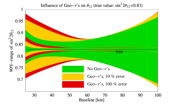
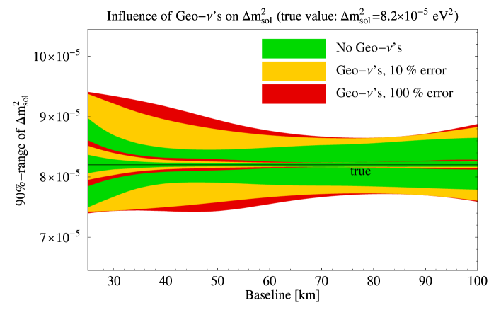
Figure 3: Achievable precision for the parameters $\sin^{2}2\theta_{12}$ (upper panel) and $\Delta m_{21}^{2}$ (lower panel) at the 90% confidence level as a function of the baseline. The outer curves correspond to the SMALL scenario, while the inner ones show the achievable precision withe the LARGE scenario. The true values we have chosen are indicated by the horizontal lines.

4.2 Numerical results

Looking at Figure 3, one can see that the optimum baselines for a measurement of the solar mixing angle $\sin^{2}2\theta_{12}$ for the SMALL scenario will be around 50 to 70 km if one includes Geo-neutrinos, and a bit shorter without Geo-neutrinos (approximately 40–60 km). This is in agreement with the optimum baselines obtained for the SADO scenario in Refs. [16, 46] (where the technically different situation “large reactor – small detector” is investigated) and with our analytical estimates. Geo-neutrinos only perturb the low energy part of the spectrum up to around 3.3 MeV, which means that, if they are present, the overall sensitivity will be dominated by the high energy part. However, for high energy neutrinos the optimum baseline will be larger due to the $L/E$-dependence of the oscillation probabilities. For the LARGE scenario, all baselines are more or less equivalent, as long as one is far enough away from the reactor to be able to resolve the solar oscillation, i.e. the oscillatory disappearance “dip” in the spectrum has to be seen. For the determination of $\Delta m_{21}^{2}$, Figure 3 and Table 2 show that the optimum baseline turns out to be 47.0 km for the SMALL and 53.2 km for the LARGE scenario, as long as the Geo-neutrino background is neglected. With the inclusion of this background, the best baseline for the SMALL scenario is shifted to 75–80 km, while for the LARGE scenario, the impact of the background is less dramatic.

$\sin^{2}2\theta_{12}$		$\mathrm{L_{OPT}\,[km]}$	events/year	precision (90% CL)
SMALL	no-Geo $\nu$’s	43.5	1866 (1026)	+4.10%/-3.61%
	10% error	57.5	2853 (514)	+5.30%/-5.30%
	100% error	59.4	2828 (488)	+5.42%/-5.42%
LARGE	no-Geo $\nu$’s	40.0	27572 (26732)	+0.60%/-0.36%
	10% error	52.9	14405 (12065)	+0.60%/-0.60%
	100% error	55.0	13466 (11127)	+0.72%/-0.60%

$\Delta m_{21}^{2}$		$\mathrm{L_{OPT}\,[km]}$	events/year	precision (90% CL)
SMALL	no Geo-$\nu$’s	47.0	1655 (815)	+3.05%/-3.54%
	10% error	76.2	2729 (389)	+5.37%/-5.73%
	100% error	79.7	2717 (378)	+5.49%/-5.85%
LARGE	no Geo-$\nu$’s	53.2	12757 (11917)	+0.37%/-0.37%
	10% error	65.0	11116 (8776)	+0.37%/-0.37%
	100% error	70.0	10589 (8250)	+0.49%/-0.49%

Table 2: The achievable precision on the solar parameters $\sin^{2}2\theta_{12}$ and $\Delta m_{21}^{2}$ at the 90% confidence level. Also shown are the optimal baselines and total (signal) event rates per year for the measurements in the LARGE and SMALL scenarios. Note that for the LARGE scenario, the exact baseline is not so important since one always has extremely high rates.

To get a better overview and to get a clue of how strongly the different scenarios are influenced by Geo-neutrinos, we summarize the numerical results in Table 2. Taking into account, that our values give the 90% confidence level ranges for the solar parameters, one can easily see that already the SMALL scenario could reach values comparable to SADO [16, 46]. It is important that, for a shorter baseline, the impact of Geo-neutrinos broadens the 90% confidence level range quite strongly, even if the flux error is only taken to be 10%. Hence, for performing a reactor experiment at such baselines, it is necessary to have a good knowledge of the Geo-neutrino fluxes. This goal can be reached for example by measuring the Geo-neutrino background before turning on or after turning off the mobile reactor. However, for the LARGE scenario, one can clearly see that an amazing precision in the measurement of the solar parameters is possible, even without precise knowledge on the Geo-neutrino background. One could of course assume, that such a precision could be spoiled by the fact that the energy of a single neutrino cannot be determined better than about $1$ or $2\%$. However, note that this precision is just the limit for each single bin. Since we consider a total of 67 bins the overall precision can indeed be better. More precisely, $2\%$ is the absolute uncertainty for each bin, but since information from different bins is compared, the relative uncertainty between the bins is the main limiting factor and this can, due to the spectral information, be much less than the former one. Hence, the precision of our results is realistic for the considered scenarios.

5 Conclusions

We have performed analytical and numerical calculations to estimate the potential of reactor anti-neutrino disappearance measurements with a Large Liquid Scintillator Detector like LENA. For the measurement of the small mixing angle $\sin^{2}2\theta_{13}$, we have assumed the reactor to be mobile. This allows subsequent measurements in a near and a far position, so that many systematical uncertainties are canceled. We have distinguished between two different scenarios, a nuclear-powered ship (e.g. an icebreaker or a submarine) and a land-based mobile reactor, where the cancellation of systematical uncertainties is different. In the case of a nuclear-powered ship, detector related and source related systematical errors are eliminated, so that the $\sin^{2}2\theta_{13}$ sensitivity follows the statistical limit with increasing exposure. In the case of the land-based mobile reactor, the source related flux normalization error remains because the reactor needs to be shut down for the displacement. If an exposure of 13.5 GW kt yrs is assumed, the nuclear-powered ship scenario can provide a limit of $\sin^{2}2\theta_{13}\lesssim 0.004$ at the 90% confidence level, whereas the land-based scenario can achieve a limit of $\sin^{2}2\theta_{13}\lesssim 0.02$ with the same exposure. Furthermore, we have shown that for the nuclear-powered ship scenario the two baselines, near and far, should be chosen around the 0th oscillation minimum ($L\approx 0$ km) and 1st oscillation maximum ($L\approx 1.3$ km), while the land-based scenario yields optimal results with near and far baselines around the 1st oscillation minimum and 1st oscillation maximum. This is advantageous because the detector will be located underground, and the mobile reactor cannot be positioned in the direct neighborhood of the detector.

We have also analyzed the potential of a Large Liquid Scintillator Detector to perform precision measurements of the solar parameters $\sin^{2}2\theta_{12}$ and $\Delta m^{2}_{21}$. For this, we have compared two scenarios: a small 0.5 GW reactor (SMALL) and a large 10 GW power station (LARGE). As has previously been shown in [16], the measurement of the solar parameters is strongly influenced by the Geo-neutrino background, therefore we have implemented an accurate treatment of this background, and compared its impact for different assumptions on the systematical uncertainties. We have shown, that the SMALL scenario would favor baselines of approximately 40 to 60 km for the measurement of $\sin^{2}2\theta_{12}$ and 47 km for the measurement of $\Delta m^{2}_{21}$. The exact choice of the baseline in the LARGE scenario turned out to be less crucial, since the excellent statistics provide precise information on the energy spectrum. Even with the most conservative assumptions on the systematical uncertainties of the Geo-neutrino background, the SMALL scenario can already achieve precisions of approximately 5.4% on $\sin^{2}2\theta_{12}$ and 5.9% on $\Delta m^{2}_{21}$, while the LARGE scenario achieves precisions of approximately 0.7% on $\sin^{2}2\theta_{12}$ and 0.5% on $\Delta m^{2}_{21}$. This very good accuracy is required e.g. to test quark-lepton complementarity at a very high precision level.

References

- [1] C. L. Cowan Jr., F. Reines, F. B. Harrison, H. W. Kruse, and A. D. McGuire, Science 124(3212), 103 (1956).
- [2] C. L. Cowan and F. Reines, Nature 178(446) (156).
- [3] K. Eguchi et al. (KamLAND), Phys. Rev. Lett. 90, 021802 (2003), hep-ex/0212021.
- [4] M. Apollonio et al. (CHOOZ), Phys. Lett. B466, 415 (1999), hep-ex/9907037.
- [5] H. Minakata, H. Sugiyama, O. Yasuda, K. Inoue, and F. Suekane, Phys. Rev. D68, 033017 (2003), hep-ph/0211111.
- [6] P. Huber, M. Lindner, T. Schwetz, and W. Winter, Nucl. Phys. B665, 487 (2003), hep-ph/0303232.
- [7] K. Anderson et al. (2004), hep-ex/0402041.
- [8] F. Ardellier et al. (2004), hep-ex/0405032.
- [9] T. Marrodan-Undagoitia et al., Phys. Rev. D72, 075014 (2005), hep-ph/0511230.
- [10] L. Oberauer, F. von Feilitzsch, and W. Potzel, Nucl. Phys. Proc. Suppl. 138, 108 (2005).
- [11] J. Hecht, New Scientist 2463 (2004).
- [12] H. Minakata and A. Y. Smirnov, Phys. Rev. D70, 073009 (2004), hep-ph/0405088.
- [13] S. Choubey and W. Rodejohann, Phys. Rev. D72, 033016 (2005), hep-ph/0506102.
- [14] M. Lindner, A. Merle, and W. Rodejohann, Phys. Rev. D73, 053005 (2006), hep-ph/0512143.
- [15] M. Blennow, T. Ohlsson, and H. Snellman, Phys. Rev. D69, 073006 (2004), hep-ph/0311098.
- [16] H. Minakata, H. Nunokawa, W. J. C. Teves, and R. Zukanovich Funchal, Phys. Rev. D71, 013005 (2005), hep-ph/0407326.
- [17] V. Barger, D. Marfatia, and K. Whisnant, Int. J. Mod. Phys. E12, 569 (2003), hep-ph/0308123.
- [18] Q. R. Ahmad et al. (SNO), Phys. Rev. Lett. 89, 011301 (2002), nucl-ex/0204008.
- [19] Q. R. Ahmad et al. (SNO), Phys. Rev. Lett. 89, 011302 (2002), nucl-ex/0204009.
- [20] S. N. Ahmed et al. (SNO), Phys. Rev. Lett. 92, 181301 (2004), nucl-ex/0309004.
- [21] T. Araki et al. (KamLAND), Phys. Rev. Lett. 94, 081801 (2005), hep-ex/0406035.
- [22] L. Wolfenstein, Phys. Rev. D17, 2369 (1978).
- [23] S. P. Mikheev and A. Y. Smirnov, Sov. J. Nucl. Phys. 42, 913 (1985).
- [24] Y. Fukuda et al. (Super-Kamiokande), Phys. Rev. Lett. 81, 1562 (1998), hep-ex/9807003.
- [25] S. Fukuda et al. (Super-Kamiokande), Phys. Lett. B539, 179 (2002), hep-ex/0205075.
- [26] K. Kaneyuki (K2K), Nucl. Phys. Proc. Suppl. 145, 124 (2005).
- [27] L. Ludovici (K2K), Nucl. Phys. Proc. Suppl. 155, 160 (2006).
- [28] N. Tagg (the MINOS) (2006), hep-ex/0605058.
- [29] R. Plunkett (MINOS) (2006), presented at 3rd International Workshop on NO-VE: Neutrino Oscillations in Venice: 50 Years after the Neutrino Experimental Discovery, Venice, Italy, 7-10 Feb 2006.
- [30] G. L. Fogli, E. Lisi, A. Marrone, and D. Montanino, Phys. Rev. D67, 093006 (2003), hep-ph/0303064.
- [31] J. N. Bahcall, M. C. Gonzalez-Garcia, and C. Pena-Garay, JHEP 08, 016 (2004), hep-ph/0406294.
- [32] A. Bandyopadhyay, S. Choubey, S. Goswami, S. T. Petcov, and D. P. Roy, Phys. Lett. B608, 115 (2005), hep-ph/0406328.
- [33] M. Maltoni, T. Schwetz, M. A. Tortola, and J. W. F. Valle, New J. Phys. 6, 122 (2004), hep-ph/0405172.
- [34] J. A. Detwiler, G. Gratta, N. Tolich, and Y. Uchida, Phys. Rev. Lett. 89, 191802 (2002), hep-ex/0207001.
- [35] M. Goodman, Low energy neutrinos (2005).
- [36] K. A. Hochmuth et al. (2005), hep-ph/0509136.
- [37] S. Enomoto, Neutrino Geophysics and Observation of Geo-Neutrinos at KamLAND, Ph.D. thesis (2005).
- [38] S. Enomoto, URL http://www.awa.tohoku.ac.jp/ sanshiro/geoneutrino/spectrum/.
- [39] URL http://www.insc.anl.gov/.
- [40] URL http://www.icjt.org/nukestat/index.html.
- [41] P. Huber, J. Kopp, M. Lindner, M. Rolinec, and W. Winter (2006), hep-ph/0601266.
- [42] P. Huber, M. Lindner, and W. Winter, Comput. Phys. Commun. 167, 195 (2005), hep-ph/0407333.
- [43] H. Murayama and A. Pierce, Phys. Rev. D65, 013012 (2002), hep-ph/0012075.
- [44] P. Vogel and J. F. Beacom, Phys. Rev. D60, 053003 (1999), hep-ph/9903554.
- [45] L. Oberauer, private communication.
- [46] H. Minakata, H. Nunokawa, W. J. C. Teves, and R. Zukanovich Funchal, Nucl. Phys. Proc. Suppl. 145, 45 (2005), hep-ph/0501250.
- [47] A. Bandyopadhyay, S. Choubey, S. Goswami, and S. T. Petcov, Phys. Rev. D72, 033013 (2005), hep-ph/0410283.
- [48] F. Mantovani, L. Carmignani, G. Fiorentini, and M. Lissia, Phys. Rev. D69, 013001 (2004), hep-ph/0309013.