Two Photon Exchange Contributions to Elastic

$ep$ Scattering in the Nonlocal Field Formalism

Pankaj Jain, Satish D. Joglekar and Subhadip Mitra

Department of Physics, IIT Kanpur - 208016, India

Abstract

We construct a nonlocal gauge invariant Lagrangian to model the electromagnetic interaction of proton. The Lagrangian includes all allowed operators with dimension up to five. We compute the two photon exchange contribution to elastic electron-proton scattering using this effective nonlocal Lagrangian. The one loop calculation in this model includes the standard box and cross box diagram with the standard on-shell form of the hadron electromagnetic vertices. Besides this we find an extra contribution which depends on an unknown constant. We use experimentally extracted form factors for our calculation. We find that the correction to the reduced cross section is slightly nonlinear as a function of the photon longitudinal polarization $\varepsilon$. The non-linearity seen is within the experimental error bars of the Rosenbluth data. The final result completely explains the difference between the form factor ratio $G_{E}/G_{M}$ extracted by Rosenbluth separation technique at SLAC and polarization transfer technique at JLAB.

1 Introduction

The electromagnetic form factors $F_{1}$ and $F_{2}$ parametrize the vertex of electromagnetic interaction of a photon with an on-shell proton,

$$\Gamma_{\mu}(p,p^{\prime})=\gamma_{\mu}F_{1}(q^{2})+\frac{i\kappa_{p}}{2M_{p}}F_{2}(q^{2})\sigma_{\mu\nu}q^{\nu},$$ (1)

where $p$ and $p^{\prime}$ are the initial and final proton momenta, $M_{p}$ is the proton mass, $\kappa_{p}$ its anomalous magnetic moment and $q=p^{\prime}-p$ is the momentum transfer. The functions $F_{1}$ and $F_{2}$ are called the Dirac and Pauli form factors respectively. They are experimentally measured by elastic scattering of electrons on protons, assuming that the process is dominated by one photon exchange diagram (Fig. 1). We also define $Q^{2}=-q^{2}\geq 0$. Besides the form factors $F_{1}$ and $F_{2}$, it is also convenient to define the electric and magnetic form factors (or the Sachs form factors), $G_{E}$ and $G_{M}$ which are more suitable for experimental extraction,

$$G_{E}(Q^{2}) = F_{1}(Q^{2})-\tau\kappa_{p}F_{2}(Q^{2})$$

$$G_{M}(Q^{2}) = F_{1}(Q^{2})+\kappa_{p}F_{2}(Q^{2})$$ (2)

where $\tau=Q^{2}/4M_{p}^{2}$. At $Q^{2}=0$, $F_{1}=F_{2}=1$ and $G_{E}=G_{M}/\mu_{p}=1$, where $\mu_{p}$ is the magnetic moment of the proton. The form factor $G_{M}\approx\mu_{p}G_{D}$ where $G_{D}$ is the dipole function,

$$G_{D}={1\over(1+{Q^{2}\over 0.71})^{2}}.$$ (3)

At low momenta, $G_{E}$ is also approximately equal to $G_{D}$. At large momenta, $Q^{2}>>1$ GeV²,

$$G_{M},F_{1}\propto{1\over Q^{4}}.$$ (4)

The experimental status of $G_{E}$ and $F_{2}$ is, however, currently unclear at large momentum transfer.

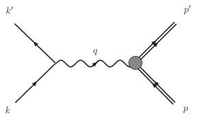
Figure 1: The one photon exchange diagram contributing to the elastic electron proton scattering. Here $k$, $k^{\prime}$ refer to the initial and final electron momenta and $p$, $p^{\prime}$ to the initial and final proton momenta respectively. $q=k-k^{\prime}=p^{\prime}-p$ is the momentum exchanged.

A standard technique for the extraction of the proton form factors is the Rosenbluth separation [2]. Here one considers the unpolarized elastic scattering of electrons on target protons. In the one photon exchange approximation the cross section can be written as

$${d\sigma\over d\Omega}={\sigma_{\rm Mott}\over\varepsilon(1+\tau)}\left[\tau G_{M}^{2}(Q^{2})+\varepsilon G_{E}^{2}(Q^{2})\right]$$ (5)

where $\varepsilon=1/[1+2(1+\tau)\tan^{2}(\theta_{e}/2)]$ is the longitudinal polarization of the photon and $\theta_{e}$ is the electron scattering angle. One finds that the reduced cross section, $\sigma_{R}=\tau G_{M}^{2}(Q^{2})+\varepsilon G_{E}^{2}(Q^{2})$ depends linearly on $\varepsilon$. By making a linear fit to the observed $\sigma_{R}$ as a function $\varepsilon$ at fixed $Q^{2}$, one can, therefore, extract both $G_{M}$ and $G_{E}$. At large $Q^{2}$, $G_{M}$ dominates at all values of $\varepsilon$. Hence the uncertainty in the extraction of $G_{E}$ can be large at large $Q^{2}$. Recent results for Rosenbluth separation are available from SLAC [3, 4] and JLAB [5]. The SLAC data shows that ${\mu_{p}G_{E}\over G_{M}}\approx 1$ upto momentum transfer $Q^{2}\approx 6$ GeV². The JLAB data is available at $Q^{2}=2.64,3.20$ and 4.10 GeV² and shows a similar trend. This result also implies that the ratio $F_{2}/F_{1}\propto 1/Q^{2}$.

A direct extraction of the ratio $G_{E}/G_{M}$ is possible by elastic scattering of longitudinally polarized electrons on target proton $\vec{e}+p\rightarrow e+\vec{p}$ [6]. In the one-photon exchange approximation, the recoiling proton acquires only two polarization components, $P_{l}$, parallel to the proton momentum and $P_{t}$, perpendicular to the proton momentum in the scattering plane. The ratio,

$${G_{E}\over G_{M}}=-{P_{t}\over P_{l}}{E_{e}+E_{e}^{\prime}\over 2M_{p}}\tan\left({\theta_{e}\over 2}\right)$$ (6)

where $E_{e}$ and $E_{e}^{\prime}$ are the energies of the initial and final electron. This technique, therefore, directly yields the ratio $G_{E}/G_{M}$. The results [7, 8, 9], available from JLAB, show $\mu_{p}G_{E}/G_{M}$ decreases with $Q^{2}$. A straight line fit to the data gives

$${\mu_{p}G_{E}\over G_{M}}\approx 1.06-0.15\,Q^{2}$$ (7)

in the momentum range $0.5<Q^{2}<5.6$ GeV². The ratio, therefore, becomes as small as 0.2 at $Q^{2}=5.6$ GeV², the maximum momentum transfer in this experiment. The polarization transfer results also imply that $QF_{2}/F_{1}\sim 1$ for $Q^{2}>1$ GeV². The observed trend in the polarization transfer experiment is, therefore, completely different from what is measured using the Rosenbluth separation. This is clearly a serious problem and has attracted considerable attention in the literature [10, 11].

2 Two Photon Exchange

An obvious source of error is the higher order corrections to the elastic scattering process. A reliable extraction of the form factors requires a careful treatment of the radiative corrections including the soft photon emission, which give a significant correction to the cross section [12, 13, 14, 15]. These contributions are calculated by keeping only the leading order terms in the soft photon momentum. Furthermore only the infrared divergent terms, which are required to cancel the divergences in the soft photon emission, are included in the radiative corrections. It is possible that the terms not included in these calculation may be responsible for the observed difference. Any such correction is likely to be small and hence cannot significantly change the results of the polarization transfer experiment. However a small correction to the Rosenbluth separation could imply a large correction to the extracted form factor $G_{E}$. A possible correction is the two photon exchange diagram which has attracted considerable attention in the literature [16, 17, 18, 19, 20]. Such a diagram is taken into account while computing the radiative corrections, but only the infrared divergent contribution is included. It is possible that the remaining contribution gives a significant correction. One may also consider next to leading order corrections in the soft photon momenta to the soft photon emission diagrams. Both of these contributions receive unknown hadronic corrections and cannot be calculated in a model independent manner.

In this paper we estimate the two photon exchange contribution using an effective non-local Lagrangian. The box and cross-box diagrams which contribute are shown in Fig. 2(a) and 2(b) respectively. As discussed later, in the non-local formalism we need to evaluate one more diagram. The two photon contribution has also been obtained by model calculations in Ref. [18, 19]. The authors find that they are able to partially reconcile the discrepancy. The results of Ref. [18, 19] show that the predicted Rosenbluth plots are no longer linear in $\varepsilon$. The experimental results obtained from JLAB [5] show very little deviation from linearity. The SLAC results [4] can incorporate some non-linearity due to the presence of relatively larger errorbars. The present limit on the deviation from linearity is given in Ref. [21]. In Ref. [20] the authors argue, using charge conjugation and crossing symmetry, that two photon exchange contribution must necessarily be nonlinear in $\varepsilon$. If the two photon exchange contribution shows large non-linearity as a function of $\varepsilon$ then it cannot provide an an explanation of the observed anomaly.

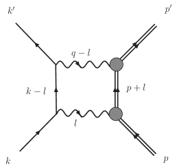
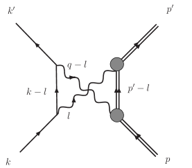
(a)	(b)

Figure 2: The two photon exchange diagrams contributing to the elastic electron proton scattering: (a) box diagram and (b) cross-box diagram.

3 General electromagnetic vertex of proton

The elementary electromagnetic vertex of an on-shell proton is given in eq. 1. When the proton is off-shell, the vertex is expected to be more general. Further, it must satisfy the WT identity, following from gauge-invariance, that implies a relation between $\Gamma_{\mu}(p,p^{\prime})$ and the inverse proton propagator, $S_{F}^{-1}(p)$. A local theory of interaction of a proton and a photon would have a $U(1)$ gauge-invariance, implied by local transformations and would imply the WT identity:

$$q^{\mu}\Gamma_{\mu}(p,p^{\prime})=S_{F}^{-1}(p^{\prime})-S_{F}^{-1}(p).$$ (8)

This identity would be violated if in calculating the two photon exchange diagrams one uses the standard on-shell form factors defined in eq. 1 and a free proton propagator. Here we are interested in formulating the theory in terms of an effective nonlocal action, which will allow us to maintain gauge invariance in the presence of form factors in the electromagnetic interaction of proton. It is certainly possible to maintain gauge invariance in a local theory also but in this case the form factors will arise only after we take into account loop corrections in strong interactions. It is not clear how to systematically do calculations in such a case. In the present case the form factors are present at the tree level interaction of photon with proton. The vertex $\Gamma_{\mu}(p,p^{\prime})$ satisfies a generalized non-local version of the WT identity:

$$g\left(q^{2}\right)q^{\mu}\Gamma_{\mu}(p,p^{\prime})=S_{F}^{-1}(p^{\prime})-S_{F}^{-1}(p).$$ (9)

where $g\left(q^{2}\right)$ is a function of $q^{2}$ appearing in the gauge-transformation equations, ultimately to be related to a form-factor in the next section. As we shall see in the next section, this identity follows from a non-local electromagnetic invariance, and in fact is more appropriate for an extended object like a proton. In the local limit, the function $g(q^{2})\rightarrow 1$, and the identity in eq. 9 reduces to the local WT identity. On account of the charge-conjugation invariance of the proton-photon interaction, the vertex $\Gamma_{\mu}(p,p^{\prime})$, a $4\times 4$ matrix, must satisfy

$$C^{-1}\Gamma_{\mu}(p,p^{\prime})C=-\Gamma_{\mu}^{T}(-p^{\prime},-p)$$ (10)

where $C$ is the charge-conjugate matrix, with $C\gamma_{\mu}C^{-1}=-\gamma_{\mu}^{T}$ [23]. We now express the vertex in its most general form, employing the 16 linearly independent Dirac matrices: $1,\gamma_{5},\gamma_{\mu},\gamma_{\mu}\gamma_{5},\sigma_{\mu\nu}$ and the 4-vectors: $P^{\mu}\equiv\left(p+p^{\prime}\right)^{\mu},q^{\mu}\equiv(p^{\prime}-p)^{\mu}$.

$$\Gamma_{\mu}(p,p^{\prime}) = aP_{\mu}+bq_{\mu}+c\gamma_{\mu}$$ (11)

$$+ d\not{P}P_{\mu}+e\not{P}q_{\mu}+f\not{q}P_{\mu}+g\not{q}q_{\mu}$$

$$+ h\sigma_{\mu\alpha}P^{\alpha}+j\sigma_{\mu\alpha}q^{\alpha}$$

$$+ k\sigma_{\alpha\beta}P^{\alpha}q^{\beta}P_{\mu}+l\sigma_{\alpha\beta}P^{\alpha}q^{\beta}q_{\mu}+m\gamma_{\alpha}\gamma_{5}\xi_{\mu}^{\nu\alpha\beta}P_{\beta}q_{\nu}.$$

Here, the 12 coefficients $a,b,....,m$ are functions of the three Lorentz invariants $p^{2},p^{\prime 2},q^{2}$. Charge conjugation requires that $a,c,d,g,j,k$ are symmetric under $p^{2}\leftrightarrow p^{\prime 2}$ and $b,e,f,h,l,m$ are antisymmetric under the same operation. To implement the WT identity, we express,

$$S_{F}^{-1}(p)=\alpha\left(p^{2}\right)\not{p}+\beta\left(p^{2}\right)$$ (12)

in its most general form. We then impose the WT identity given in eq. 9. This leads to some constraints between the coefficients. The net result of all this is to yield the following form for $\Gamma_{\mu}$:

$$\Gamma_{\mu}(p,p^{\prime})=a^{\prime}P_{\mu}+c^{\prime}\gamma_{\mu}+j\sigma_{\mu\alpha}q^{\alpha}+d^{\prime}\not{P}P_{\mu}+7\mbox{ divergence free terms}.$$

We enumerate the divergence free (i.e. $X_{\mu}$ with $q^{\mu}X_{\mu}\equiv 0$) terms:

$$b^{\prime}\left[(p^{\prime 2}-p^{2})q_{\mu}-q^{2}P_{\mu}\right]+f\left(-P.q\gamma_{\mu}+\not{q}P_{\mu}\right)+g\left(-q^{2}\gamma_{\mu}+\not{q}q_{\mu}\right)$$

$$+ k\left(-\sigma_{\mu\alpha}P^{\alpha}P.q+\sigma_{\alpha\beta}P^{\alpha}q^{\beta}P_{\mu}\right)+l\left(\sigma_{\mu\alpha}P^{\alpha}q^{2}-\sigma_{\beta\alpha}P^{\alpha}q^{\beta}q_{\mu}\right)$$

$$+ e^{\prime}\left(-q^{2}\not{P}P_{\mu}+P.q\not{P}q_{\mu}\right)+m\gamma_{\alpha}\gamma_{5}\xi_{\mu}^{\nu\alpha\beta}P_{\beta}q_{\nu}.$$

We further note the relations that arise from the WT identity and which restrict the form of some of the coefficients $(a^{\prime},c^{\prime})$ considerably:

$$a^{\prime}=\frac{\beta\left(p^{\prime 2}\right)-\beta\left(p^{2}\right)}{g\left(q^{2}\right)\left(p^{\prime 2}-p^{2}\right)};\;\;c^{\prime}=\frac{\alpha\left(p^{\prime 2}\right)+\alpha\left(p^{2}\right)}{2g\left(q^{2}\right)};\;\;d^{\prime}=\frac{\alpha\left(p^{\prime 2}\right)-\alpha\left(p^{2}\right)}{g\left(q^{2}\right)\left(p^{\prime 2}-p^{2}\right)}.$$

whereas the coefficients of $j,b,f,g,k,l,m$ are completely arbitrary functions of the Lorentz invariants. We make several observations:

1. We note first that power counting would associate all operators except those three with coefficients $a^{\prime},c^{\prime},j$ with a local operator of dimension 6 or higher.

2. We note that the dependence on $q^{2}$ of both $a^{\prime}$ and $c^{\prime}$ are identical. Near mass-shell, $\alpha\left(p^{2}\right)\sim\alpha_{0}+\alpha_{1}[p^{2}-M_{p}^{2}],\,\,\beta\left(p^{2}\right)\sim\beta_{0}+\beta_{1}[p^{2}-M_{p}^{2}]$; and thus,

   $$a^{\prime} = \left\{\beta_{1}+\mathcal{O}[p^{2}-M_{p}^{2}]\right\}g^{-1}\left(q^{2}\right);\,\,$$

   $$c^{\prime} = \left\{\alpha_{0}+\frac{1}{2}\alpha_{1}[p^{2}+p^{\prime 2}-2M_{p}^{2}]\right\}g^{-1}\left(q^{2}\right).$$ (13)

3. The on-shell expression (eq. 1) for $\Gamma_{\mu}(p,p^{\prime})$ takes operators of dimensions 4 (electric) and 5 (magnetic) into account. It is then logical that the only other operator of dimensions 5 should also be included in the off-shell expression for the $\Gamma_{\mu}(p,p^{\prime})$. We shall take these three terms into account in our minimal effective Lagrangian model.

4 Effective Lagrangian Model

We represent the interaction of the photon-proton system by an effective nonlocal Lagrangian model based on the discussion in the last section. We adopt the following guidelines in the process:

• The Lagrangian model should incorporate up to dimension 5 operators, for reasons partly explained in the previous section. The assumption is that in the effective Lagrangian approach, the higher dimension operators will contribute much less. This is borne out in the calculations performed. (See Figure 15 and the subsequent discussion.)

• The model should incorporate the results regarding the form of the coefficients $a^{\prime},c^{\prime}$ obtained earlier (see eq. 13), thus at least embody the form-factors on mass-shell. The resulting model is necessarily non-local.

• We assume that the model has lowest order derivatives of fermions. Our assumption about the dimensionality of operators is consistent with this.

• We require that this non-local model has an equivalent form of gauge-invariance. Such constructions of non-local versions of local symmetries are known in literature [24, 22] and we shall show explicitly that our model below has a very simple form of non-local gauge-invariance.

A Lagrangian model which satisfies these constraints is given by,

$$\mathcal{L=\overline{\psi}}\left(i\not{\partial}-ef^{\prime}_{1}\left[\frac{\partial^{2}}{\Lambda^{2}}\right]\not{A}-M_{p}\right)\psi+\frac{a^{\prime\prime}}{2M_{p}}\mathcal{\overline{\psi}}\left(\sigma_{\mu\nu}f^{\prime}_{2}\left[\frac{\partial^{2}}{\Lambda^{2}}\right]F^{\mu\nu}\right)\psi\\ +\frac{b^{\prime\prime}}{2M_{p}}\mathcal{\overline{\psi}}\widetilde{D}^{2}\psi$$

where $i\widetilde{D}=i\partial-ef^{\prime}_{1}\left[\frac{\partial^{2}}{\Lambda^{2}}\right]A$ is the non-local covariant derivative. We point out that the form factors, $f^{\prime}_{1}$ and $f_{2}^{\prime}$ are to be extracted directly from experiments. We make a number of observations regarding this effective Lagrangian:

1. $\mathcal{L}$ is invariant under the non-local form of gauge transformations:

   $$\delta A_{\mu}=-\partial_{\mu}\alpha\left(x\right);\psi(x)\rightarrow e^{ief^{\prime}_{1}\left[\frac{\partial^{2}}{\Lambda^{2}}\right]\alpha\left(x\right)}\psi(x),\overline{\psi}(x)\rightarrow\overline{\psi}(x)e^{-ief^{\prime}_{1}\left[\frac{\partial^{2}}{\Lambda^{2}}\right]\alpha\left(x\right)}$$

   or equivalently,

   $$\delta A_{\mu}=-\partial_{\mu}f^{\prime-1}_{1}\left[\frac{\partial^{2}}{\Lambda^{2}}\right]\beta\left(x\right);\psi(x)\rightarrow e^{ie\beta\left(x\right)}\psi(x),\overline{\psi}(x)\rightarrow\overline{\psi}(x)e^{-ie\beta\left(x\right)}$$

   In the latter form, the gauge transformations are similar to the usual local ones, with the exception that in the first of these $\partial_{\mu}\rightarrow\partial_{\mu}f^{\prime-1}_{1}\left(\frac{\partial^{2}}{\Lambda^{2}}\right)$. This leads to the non-local WT identity of eq. 9; i.e., with a replacement $q_{\mu}\rightarrow q_{\mu}f^{\prime-1}_{1}\left(\frac{-q^{2}}{\Lambda^{2}}\right)\equiv q_{\mu}g(q^{2})$ in eq. 8. Under this transformation, $F^{\mu\nu}$ and hence the second term is gauge-invariant independent of the form of $f^{\prime}_{2}$. Also, the non-local gauge-covariant derivative satisfies: $\widetilde{D}\psi\rightarrow e^{ie\beta\left(x\right)}\widetilde{D}\psi(x)$.

2. The last term generates a term proportional to $P_{\mu}$ in $\Gamma_{\mu}(p,p^{\prime})$ with a form factor proportional to $f^{\prime}_{1}$, the same one appearing in the electric term. This is consistent with the comment on the form of $a^{\prime}$ and $c^{\prime}$ given earlier.

3. The (non-local) gauge-invariance of the last term requires that it is composed of the (non-local) gauge-covariant derivative: this restricts the form-factor present in this term as above.

4. The Lagrangian is exactly valid as long as the proton is on-shell, irrespective of the value of the momentum transfer $q^{2}$. In this limit the interaction of the proton with photon is described in terms of the two form factors and no higher dimensional terms are required. The higher derivative terms we drop give higher order contributions in powers of $(P^{2}-M_{p}^{2})/\Lambda^{2}$, where $P^{2}-M_{p}^{2}$ is the offshellness of proton momentum. These higher order terms can be dropped as long as the dominant contribution to a process is obtained from the kinematic region where $(P^{2}-M_{p}^{2})/\Lambda^{2}<<1$.

5. In the limit $\Lambda\rightarrow\infty$ we reproduce the local field theory model for a proton with an anomalous magnetic moment.

Before we proceed, a comment on the non-local form of gauge-invariance is in order. It appears that a local form of gauge-invariance for extended particles such as a proton is inappropriate. Consider the wave-function of an extended particle centered at $\mathbf{x}$: viz. $\psi(\mathbf{x,}t)$. Let $\mathbf{y}$ be a point within the charge-radius $R$ of the proton: $|\mathbf{x-y}|<R$. Let us imagine that a gauge-transformation on $A_{\mu}$ is carried out (at $t$) around $\mathbf{y}$ with a very narrow support, $\rho:\rho<<|\mathbf{x-y}|$. In the model of fundamental constituents, the quark wave-function should be affected around $\mathbf{y}$, which in turn should affect the proton wave-function even though the gauge-transformation at $\mathbf{x}$, depending on $\alpha\left(x\right)$ will be zero. Thus, the proton wave-function should be affected by a local gauge-transformation with a support anywhere in its charge radius. The above form of non-local version of gauge-transformations embodies this idea. Note that the Fourier transform of $f^{\prime}_{1}\left[\frac{\partial^{2}}{\Lambda^{2}}\right]$ has a support over a distance $\sim 1/\Lambda\sim R$.

It proves convenient to rearrange the Lagrangian as follows (Recall the relation $\not{D}^{2}=D^{2}+\frac{e}{2}\sigma_{\mu\nu}F^{\mu\nu}$):

$$\mathcal{L=\overline{\psi}}\left(i\not{\widetilde{D}}-M_{p}\right)\psi+\frac{\tilde{a}}{2M_{p}}\mathcal{\overline{\psi}}\left(\sigma_{\mu\nu}f^{\prime}_{2}\left[\frac{\partial^{2}}{\Lambda^{2}}\right]F^{\mu\nu}\right)\psi\\ +\frac{\bar{b}}{2M_{p}}\mathcal{\overline{\psi}}\,\left(i\not{\widetilde{D}}-M_{p}\right)^{2}\psi$$

Had there been no magnetic term, the last term would have formally vanished by classical equation of motion. We note that an inclusion of the last term has now modified the inverse propagator: it has non-vanishing terms at $e=0$. This, in particular, gives a spurious pole in the propagator at another value of $\not{p}$. This problem can be avoided if we can write the $\mathcal{L}$ in the following form:

$$\mathcal{L=\overline{\psi}}\left(i\not{\widetilde{D}}-M_{p}\right)exp\left\{\frac{\bar{b}}{2M_{p}}\left(i\not{\widetilde{D}}-M_{p}\right)\right\}\psi+\frac{\bar{a}}{2M_{p}}\mathcal{\overline{\psi}}\left(\sigma_{\mu\nu}f^{\prime}_{2}\left[\frac{\partial^{2}}{\Lambda^{2}}\right]F^{\mu\nu}\right)\psi$$ (14)

which is now understood to have been consistently truncated to a given order in $\bar{b}$. We now note that the inverse propagator is:

$$\left(\not{p}-M_{p}\right)exp\left\{\frac{\bar{b}}{2M_{p}}\left(\not{p}-M_{p}\right)\right\}$$

and has only one zero at $\not{p}-M_{p}=0$ and the residue of the propagator at the pole is $1$. (In this form of $\mathcal{L}$, $\bar{a}$ is related to the anomalous magnetic moment, $\kappa_{p}$ by the relation, $\bar{a}=e\kappa_{p}/2$ and $M_{p}$ is the physical mass). Since we shall consider, in the two photon exchange calculation, terms with the last operator of dimension 5 inserted in two photon vertices, we shall do the entire calculation consistently to $O\left({\bar{b}}^{2}\right)$ using eq. 14. In this case, the propagator for the proton is

$$\frac{i}{\not{p}-M_{p}}\,exp\left\{-\frac{\bar{b}}{2M_{p}}\left(\not{p}-M_{p}\right)\right\}\approx\frac{i}{\not{p}-M_{p}}-\frac{i\bar{b}}{2M_{p}}+\frac{i{\bar{b}}^{2}}{8M_{p}^{2}}\left(\not{p}-M_{p}\right)$$

5 Reduction of the action

In this section, we shall find an effective way to calculate the matrix elements involving insertion of the last term in the action. Since a 2-photon exchange diagram at 1-loop is at most $\mathcal{O}[{\bar{b}}^{2}]$, we shall evaluate the effect of this term to $\mathcal{O}[{\bar{b}}^{2}]$ . What we are interested in are the tree-order matrix elements of two (possibly virtual) photon emission from an on-shell proton. The calculation of these can be simplified considerably in this context with the use of the fermion equations of motion. The result is simple: of all the terms up to $\mathcal{O}[{\bar{b}}^{2}]$, viz. $\mathcal{O}[\bar{b},\bar{b}\bar{a},{\bar{b}}^{2},{\bar{b}}^{2}\bar{a},{\bar{b}}^{2}{\bar{a}}^{2}]$, only the last term of $\mathcal{O}[{\bar{b}}^{2}{\bar{a}}^{2}]$ gives a non-zero result. While the result can be worked out, it is most effectively dealt with in the path-integral formulation.

We define,

$$W[J^{\mu},K,\overline{K}]=\int D\phi\exp i\left\{\int d^{4}x[\mathcal{L}+J^{\mu}A_{\mu}+\overline{K}\psi+\overline{\psi}K\right\}$$

where $\mathcal{L}$ is the action of eq. 14 and $D\phi$ denotes generically the measure of the path-integral. We now perform a field transformation:

$$\psi=\exp\left\{-\frac{\bar{b}}{2M_{p}}\left(i\not{\widetilde{D}}-M_{p}\right)\right\}\psi^{\prime}$$ (15)

Under this transformation, the Jacobian is,

$$J = \det\exp\left\{-\frac{\bar{b}}{2M_{p}}\left(i\not{\widetilde{D}}-M_{p}\right)\right\}=\exp tr\left\{-\frac{\bar{b}}{2M_{p}}\left(i\not{\widetilde{D}}-M_{p}\right)\right\}$$ (16)

$$= \exp tr\left\{\frac{\bar{b}}{2}\mathcal{I}\right\}=\mbox{a constant.}$$

and hence can be ignored for the connected Green’s functions. This then yields,

$$W[J^{\mu},K,\overline{K}]$$

$$= \int D\phi\exp i\Bigg{\{}\int d^{4}x\left[\mathcal{\overline{\psi}}\left(i\not{\widetilde{D}}-M_{p}\right)\psi^{\prime}+\frac{\bar{a}}{2M_{p}}\mathcal{\overline{\psi}}\left(\sigma_{\mu\nu}f^{\prime}_{2}\left[\frac{\partial^{2}}{\Lambda^{2}}\right]F^{\mu\nu}\right)\right.$$

$$\times \left.\exp\left\{-\frac{\bar{b}}{2M_{p}}\left[i\not{\widetilde{D}}-M_{p}\right]\right\}\psi^{\prime}\right]\ \Bigg{\}}\times\exp i\Bigg{\{}\int d^{4}x\biggl{[}J^{\mu}A_{\mu}+\overline{\psi}K$$

$$+ \left.\overline{K}\exp\left\{-\frac{\bar{b}}{2M_{p}}\left[i\not{\widetilde{D}}-M_{p}\right]\right\}\psi^{\prime}\right]\ \Bigg{\}}$$

We note that if we had $\bar{a}=0$, we would have no left-over term in the action. It is easy to show that $\overline{K}\left[\exp\left\{-\frac{\bar{b}}{2M_{p}}\left[i\not{\widetilde{D}}-M_{p}\right]\right\}-1\right]\psi^{\prime}$ does not contribute to tree-level on-shell proton matrix elements. Thus all tree-level on-shell 2-proton matrix elements involving the last term in eq. 14 are at least of order $\bar{a}\bar{b}$. We now expand the action to $\mathcal{O}[{\bar{b}}^{2}]$. We find,

$$W[J^{\mu},K,\overline{K}]=\int D\phi\exp i\left\{\int d^{4}x\left[\mathcal{L}^{\prime}+J^{\mu}A_{\mu}+\overline{K}\psi^{\prime}+\overline{\psi}K\right]\right\}+\mathcal{O}[{\bar{b}}^{3}]$$

with

$$\mathcal{L}^{\prime} = \left[\mathcal{\overline{\psi}}+\frac{\bar{a}}{2M_{p}}\mathcal{\overline{\psi}}\left(\sigma_{\mu\nu}f^{\prime}_{2}\left[\frac{\partial^{2}}{\Lambda^{2}}\right]F^{\mu\nu}\right)\left\{-\frac{\bar{b}}{2M_{p}}\right.\right.+\left.\left.\frac{{\bar{b}}^{2}}{8M_{p}^{2}}\left(i\not{\widetilde{D}}-M_{p}\right)\right\}\right]\left(i\not{\widetilde{D}}-M_{p}\right)\psi^{\prime}$$

$$+ \frac{\bar{a}}{2M_{p}}\mathcal{\overline{\psi}}\left(\sigma_{\mu\nu}f^{\prime}_{2}\left[\frac{\partial^{2}}{\Lambda^{2}}\right]F^{\mu\nu}\right)\psi^{\prime}$$

We now perform another field transformation,

$$\mathcal{\overline{\psi}}+\frac{\bar{a}}{2M_{p}}\mathcal{\overline{\psi}}\left(\sigma_{\mu\nu}f^{\prime}_{2}\left[\frac{\partial^{2}}{\Lambda^{2}}\right]F^{\mu\nu}\right)\left\{-\frac{\bar{b}}{2M_{p}}+\frac{{\bar{b}}^{2}}{8M_{p}^{2}}\left(i\not{\widetilde{D}}-M_{p}\right)\right\}=\mathcal{\overline{\psi}}^{\prime}\equiv\mathcal{\overline{\psi}}[1+X]$$ (17)

We can write,

$$\overline{\psi} = \mathcal{\overline{\psi}}^{\prime}\left\{1+\frac{\bar{a}}{2M_{p}}\sigma_{\mu\nu}f^{\prime}_{2}\left[\frac{\partial^{2}}{\Lambda^{2}}\right]F^{\mu\nu}\left\{-\frac{\bar{b}}{2M_{p}}+\frac{{\bar{b}}^{2}}{8M_{p}^{2}}\left(i\not{\widetilde{D}}-M_{p}\right)\right\}\right\}^{-1}$$

$$= \mathcal{\overline{\psi}}^{\prime}+\mathcal{\overline{\psi}}^{\prime}\left(-\frac{\bar{a}}{2M_{p}}\right)\sigma_{\mu\nu}f^{\prime}_{2}\left[\frac{\partial^{2}}{\Lambda^{2}}\right]F^{\mu\nu}\left\{-\frac{\bar{b}}{2M_{p}}+\frac{{\bar{b}}^{2}}{8M_{p}^{2}}\left(i\not{\widetilde{D}}-M_{p}\right)\right\}+\mathcal{O}[F^{2}]$$

The $\mathcal{O}[F^{2}]$ will not matter for the present calculation of 2-photon exchange, as it will give a term having 3-photon fields. The Jacobean for this transformation,

$$1/J^{\prime} = \det[1+X]=\det\left[1+X+\frac{X^{2}}{2}-\frac{X^{2}}{2}+\mathcal{O}[{\bar{b}}^{3}]\right]$$

$$= \det\left[e^{X}-\frac{X^{2}}{2}+\mathcal{O}[{\bar{b}}^{3}]\right]=\det e^{X}\det\left[1-e^{-X}\frac{X^{2}}{2}+\mathcal{O}[{\bar{b}}^{3}]\right]$$

$$= \exp[trX]\det\left[1-e^{-X}\frac{X^{2}}{2}\right]=1-tr\left(e^{-X}\frac{X^{2}}{2}\right)+\mathcal{O}[{\bar{b}}^{3}]$$

$$= 1-tr\frac{X^{2}}{2}+\mathcal{O}[{\bar{b}}^{3}]$$

$$= 1-\frac{{\bar{a}}^{2}{\bar{b}}^{2}}{32M_{p}^{4}}f^{\prime}_{2}\left[\frac{\partial^{2}}{\Lambda^{2}}\right]F_{\mu\nu}f^{\prime}_{2}\left[\frac{\partial^{2}}{\Lambda^{2}}\right]F^{\mu\nu}\times\mbox{(constant)}$$

The last term does not contribute to the emission of two photons from a proton line in the tree approximation. As a result of the transformation (eq. 17), the action then becomes,

$$\mathcal{L}^{\prime\prime} = \mathcal{\overline{\psi}}^{\prime}\left(i\not{\widetilde{D}}-M_{p}\right)\psi^{\prime}+\frac{\bar{a}}{2M_{p}}\mathcal{\overline{\psi}}^{\prime}\left(\sigma_{\mu\nu}f^{\prime}_{2}\left[\frac{\partial^{2}}{\Lambda^{2}}\right]F^{\mu\nu}\right)\psi^{\prime}$$

$$+ \left(\frac{\bar{a}}{2M_{p}}\right)^{2}\left(\frac{\bar{b}}{2M_{p}}\right)\mathcal{\overline{\psi}}^{\prime}\left(\sigma_{\mu\nu}f^{\prime}_{2}\left[\frac{\partial^{2}}{\Lambda^{2}}\right]F^{\mu\nu}\right)^{2}\psi^{\prime}$$

$$- \left(\frac{\bar{a}}{2M_{p}}\right)^{2}\left(\frac{\bar{b}^{2}}{8M_{p}^{2}}\right)\mathcal{\overline{\psi}}^{\prime}\left(\sigma_{\mu\nu}f^{\prime}_{2}\left[\frac{\partial^{2}}{\Lambda^{2}}\right]F^{\mu\nu}\right)\left(i\not{\widetilde{D}}-M_{p}\right)\left(\sigma_{\mu\nu}f^{\prime}_{2}\left[\frac{\partial^{2}}{\Lambda^{2}}\right]F^{\mu\nu}\right)\psi^{\prime}+\mathcal{O}[\bar{b}^{3}]$$

and the source term transforms into

$$\overline{\psi}^{\prime}[1+X]^{-1}K = \overline{\psi}^{\prime}\left\{1+\left(-\frac{\bar{a}}{2M_{p}}\right)\sigma_{\mu\nu}f^{\prime}_{2}\left[\frac{\partial^{2}}{\Lambda^{2}}\right]F^{\mu\nu}\left\{-\frac{\bar{b}}{2M_{p}}+\frac{\bar{b}^{2}}{8M_{p}^{2}}\left(i\not{\widetilde{D}}-M_{p}\right)\right\}\right\}K$$

$$+ \overline{\psi}^{\prime}\left(\frac{\bar{a}}{2M_{p}}\right)\,\left(\frac{\bar{b}^{2}}{8M_{p}^{2}}\right)\sigma_{\mu\nu}f^{\prime}_{2}\left[\frac{\partial^{2}}{\Lambda^{2}}\right]F^{\mu\nu}\sigma_{\mu\nu}f^{\prime}_{2}\left[\frac{\partial^{2}}{\Lambda^{2}}\right]F^{\mu\nu}K$$

None of these terms contribute to the tree approximation 2-photon matrix element for reasons similar as before.

In conclusion, when we look at the 2-photon exchange diagrams having up to two insertions of the last term in eq. 4, each set of diagrams contain a common part, viz., two (unphysical)-photon tree amplitude from an on-shell proton. The above discussion shows that the net effect of that comes from the terms

$$\left(\frac{\bar{a}}{2M_{p}}\right)^{2}\left(\frac{\bar{b}}{2M_{p}}\right)\mathcal{\overline{\psi}}^{\prime}\left(\sigma_{\mu\nu}f^{\prime}_{2}\left[\frac{\partial^{2}}{\Lambda^{2}}\right]F^{\mu\nu}\right)^{2}\psi^{\prime}$$ (18)

$$- \left(\frac{\bar{a}}{2M_{p}}\right)^{2}\left(\frac{\bar{b}^{2}}{8M_{p}^{2}}\right)\mathcal{\overline{\psi}}^{\prime}\left(\sigma_{\mu\nu}f^{\prime}_{2}\left[\frac{\partial^{2}}{\Lambda^{2}}\right]F^{\mu\nu}\right)\left(i\not{\widetilde{D}}-M_{p}\right)\left(\sigma_{\mu\nu}f^{\prime}_{2}\left[\frac{\partial^{2}}{\Lambda^{2}}\right]F^{\mu\nu}\right)\psi^{\prime}$$

We shall show in appendix 1 that the first term does not contribute in the Feynman gauge. That leaves us with only the last term. The Feynman diagram corresponding to this term is shown in Fig. 3.

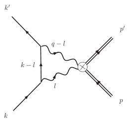
Figure 3: The two photon exchange diagram proportional to $\bar{b}^{2}$ contributing to the elastic electron proton scattering. The Feynman rule for this diagram can be obtained from eq. 18.

6 Calculation and Results

In this section we give details of the calculation of the two photon exchange diagrams using our effective Lagrangian. The calculation turns out to be complicated due to the explicit presence of form factors at the vertices. We also require models for the form factors both in the space-like and time-like regions. In the space like region the form factor $F_{1}(q^{2})$ is known reasonably well. In the time like region experimental data exists for the form factor $G_{M}(q^{2})$ for $4M_{p}^{2}<q^{2}<14$ GeV², where $4M_{p}^{2}$ is the threshold energy for $p\bar{p}$ production. In Ref. [25], $G_{M}(q^{2})$ has been extracted in the unphysical region $0<q^{2}<4M_{p}^{2}$ by using dispersion relations [26, 27]. The extracted form factor shows two resonances at masses $M\sim 770$ MeV and $M\sim 1600$ MeV. The phase of the magnetic form factor also shows a large variation in the unphysical region. The electric form factor $G_{E}(q^{2})$, however, is not well known. The amplitude in the unphysical region is obtained in Ref. [28]. However the phase is not known. Our model for the form factors is given in Appendix 2. We use two different models. Both consist of a sum of simple poles. The corresponding masses and widths are given in Tables 3 and 4. The values of these parameters are obtained by fits to the experimental data, or the data obtained from experiments by using dispersion relations [25]. The resulting amplitude and phase of the form factors for the two models are shown in Fig. 4 and 5 respectively.

Figure 4: The amplitude of $G_{M}/\mu_{p}$ (solid line) and $G_{E}$ (dotted line - Model I, dashed line - Model II). The unfilled squares represent the constrained values for $G_{E}$ at $q^{2}=0$ and $q^{2}=4M^{2}$. Results of Rosenbluth extraction experiments (filled circles - JLAB, unfilled circles - SLAC) are also shown.

Figure 5: The phase (in degrees) of $G_{M}$ (solid line) and $G_{E}$ (dotted line - Model I, dashed line - Model II).

Using these models for the magnetic and electric form factors we can obtain the form factors $F_{1}$ and $F_{2}$, required for our calculation. The models used are convenient since they allow us to use the Feynman parametrization to compute the loop integrals. The form factors for the two models have a small imaginary part even for space like momenta. However this region contributes negligibly to the loop integrals. The dominant contribution comes from the unphysical region $0<q^{2}<4M_{p}^{2}$ where the form factor is several orders of magnitude larger than its value in the space like region. In this region our model provides a very good fit to the extracted form factor [25]. Moreover the imaginary part in space like region is very small and unlikely to affect our results significantly. The resulting amplitudes and phases for model I are shown in Figs. 6 and 7 respectively. The corresponding results for model II are shown in Figs. 8 and 9.

Figure 6: The amplitude of $F_{1}$ (solid line) and $F_{2}$ (dashed line) - Model I.

Figure 7: The phase (in degrees) of $F_{1}$ (solid line) and $F_{2}$ (dashed line) - Model I.

Figure 8: The amplitude of $F_{1}$ (solid line) and $F_{2}$ (dashed line) - Model II.

Figure 9: The phase (in degrees) of $F_{1}$ (solid line) and $F_{2}$ (dashed line) - Model II.

Using the form factor models in Appendix 2 we can determine the amplitudes of the box and cross box diagram as well as the amplitude due to the extra term displayed in eq. 18. The box diagram amplitude can be written as,

$$i\mathcal{M}_{B} = e^{4}\sum_{a,b}\int\frac{d^{4}l}{(2\pi)^{4}}\frac{\bar{u}(k^{\prime})\gamma^{\mu}(\not{k}-\not{l})\gamma^{\nu}u(k)}{((k-l)^{2}-m_{e}^{2}+i\xi)(l^{2}-\mu^{2}+i\xi)(\tilde{q}^{2}-\mu^{2}+i\xi)}$$ (19)

$$\times \left[\bar{U}(p^{\prime})\{F_{1}(\tilde{q})\gamma_{\mu}+i\frac{\kappa_{p}}{2M_{p}}F_{2}(\tilde{q})\sigma_{\mu\alpha}(\tilde{q})^{\alpha}\}\right.\frac{\not{p}+\not{l}+M_{p}}{(p+l)^{2}-M_{p}^{2}+i\xi}$$

$$\times \left.\{F_{1}(l)\gamma_{\nu}+i\frac{\kappa_{p}}{2M_{p}}F_{2}(l)\sigma_{\nu\beta}l^{\beta}\}U(p)\right],$$

where $\tilde{q}=q-l$, $m_{e}$ is the mass of the electron and $\xi$ is an infinitesimal positive parameter. A small mass of the photon $\mu$ has been introduced in order to regulate the infrared divergence in these integrals. The infrared divergent part has to be subtracted from our result since it is included in the standard radiative corrections which are applied while extracting the form factor. Using the form factor model in Appendix 2, we find,

$$i\mathcal{M}_{B} = e^{4}\sum_{a,b}\int\frac{d^{4}l}{(2\pi)^{4}}\frac{\bar{u}(k^{\prime})\gamma^{\mu}(\not{k}-\not{l})\gamma^{\nu}u(k)}{((k-l)^{2}-m_{e}^{2}+i\xi)(l^{2}-\mu^{2}+i\xi)(\tilde{q}^{2}-\mu^{2}+i\xi)}$$ (20)

$$\times \left[\bar{U}(p^{\prime})\{(C_{a}g_{a}(\tilde{q})-4M_{p}^{2}D_{a}\tilde{g_{a}}(\tilde{q}))\gamma_{\mu}+i2M_{p}D_{a}\tilde{g_{a}}(\tilde{q})\sigma_{\mu\alpha}(\tilde{q})^{\alpha}\}\right.\frac{\not{p}+\not{l}+M_{p}}{(p+l)^{2}-M_{p}^{2}+i\xi}$$

$$\times \left.\{(C_{b}g_{b}(l)-4M_{p}^{2}D_{b}\tilde{g_{b}}(l))\gamma_{\nu}+i2M_{p}D_{b}\tilde{g_{b}}(l)\sigma_{\nu\beta}l^{\beta}\}U(p)\right].$$

It is convenient to rewrite this expression in terms of the coefficients $C^{\prime}$ and $D^{\prime}$, defined in Appendix 2. We find,

$$i\mathcal{M}_{B} = e^{4}\sum_{i,j}\int\frac{d^{4}l}{(2\pi)^{4}}\left[\frac{\bar{u}(k^{\prime})\gamma^{\mu}(\not{k}-\not{l})\gamma^{\nu}u(k)}{(k-l)^{2}-m_{e}^{2}+i\xi}\right]$$ (22)

$$\times\left[\bar{U}(p^{\prime})\{(C^{\prime}_{i}g_{i}(\tilde{q})-4M_{p}^{2}D^{\prime}_{i}g_{i}(\tilde{q}))\gamma_{\mu}+i2M_{p}D^{\prime}_{i}g_{i}(\tilde{q})\sigma_{\mu\alpha}(\tilde{q})^{\alpha}\}\right.\frac{\not{p}+\not{l}+M_{p}}{(p+l)^{2}-M_{p}^{2}+i\xi}$$

$$\times\left.\{(C^{\prime}_{j}g_{j}(l)-4M_{p}^{2}D^{\prime}_{j}g_{j}(l))\gamma_{\nu}+i2M_{p}D^{\prime}_{j}g_{j}(l)\sigma_{\nu\beta}l^{\beta}\}U(p)\right]$$

$$\equiv e^{4}\int\frac{d^{4}l}{(2\pi)^{4}}\frac{1}{((k-l)^{2}-m_{e}^{2}+i\xi)((p+l)^{2}-M_{p}^{2}+i\xi)}$$

$$\times\sum_{i,j}\left[n_{1}(C^{\prime}_{i},D^{\prime}_{i},C^{\prime}_{j},D^{\prime}_{j})+l^{4}n_{2}(C^{\prime}_{i},D^{\prime}_{i},C^{\prime}_{j},D^{\prime}_{j})\right]$$

where the last step defines the factors $n_{1}(C^{\prime}_{i},D^{\prime}_{i},C^{\prime}_{j},D^{\prime}_{j})$ and $n_{2}(C^{\prime}_{i},D^{\prime}_{i},C^{\prime}_{j},D^{\prime}_{j})$. We may cancel the $l^{2}$ factor multiplying $n_{2}(C^{\prime}_{i},D^{\prime}_{i},C^{\prime}_{j},D^{\prime}_{j})$ with a factor ($l^{2}-\mu^{2}+i\xi$) in the denominator. We then find,

$$i\mathcal{M}_{B} = e^{4}\int\frac{d^{4}l}{(2\pi)^{4}}\frac{1}{((k-l)^{2}-m_{e}^{2}+i\xi)((p+l)^{2}-M_{p}^{2}+i\xi)}$$ (23)

$$\times\sum_{i,j}\left[n_{1}(C^{\prime}_{i}D^{\prime}_{i},C^{\prime}_{j},D^{\prime}_{j})+l^{2}n_{2}(C^{\prime}_{i},D^{\prime}_{i},C^{\prime\prime}_{j},D^{\prime\prime}_{j})\right].$$

The cross-box diagram amplitude can be written as,

$$i\mathcal{M}_{CB} = e^{4}\sum_{a,b}\int\frac{d^{4}l}{(2\pi)^{4}}\left[\frac{\bar{u}(k^{\prime})\gamma^{\mu}(\not{k}-\not{l})\gamma^{\nu}u(k)}{(k-l)^{2}-m_{e}^{2}+i\xi}\right]\left[\frac{1}{(l^{2}-\mu^{2}+i\xi)(\tilde{q}^{2}-\mu^{2}+i\xi)}\right]$$ (24)

$$\times \left[\bar{U}(p^{\prime})\{F_{1}(l)\gamma_{\nu}+i\frac{\kappa_{p}}{2M_{p}}F_{2}(l)\sigma_{\nu\beta}l^{\beta}\}\right.\frac{\not{p}+\not{q}-\not{l}+M_{p}}{(p+\tilde{q})^{2}-M_{p}^{2}+i\xi}$$

$$\times \left.\{F_{1}(\tilde{q})\gamma_{\mu}+i\frac{\kappa_{p}}{2M_{p}}F_{2}(\tilde{q})\sigma_{\mu\alpha}(\tilde{q})^{\alpha}\}U(p)\right]$$

$$= e^{4}\sum_{a,b}\int\frac{d^{4}l}{(2\pi)^{4}}\left[\frac{\bar{u}(k^{\prime})\gamma^{\mu}(\not{k}-\not{l})\gamma^{\nu}u(k)}{(k-l)^{2}-m_{e}^{2}+i\xi}\right]\left[\frac{1}{(l^{2}-\mu^{2}+i\xi)(\tilde{q}^{2}-\mu^{2}+i\xi)}\right]$$

$$\times \left[\bar{U}(p^{\prime})\{(C_{b}g_{b}(l)-4M_{p}^{2}D_{b}\tilde{g_{b}}(l))\gamma_{\nu}+i2M_{p}D_{b}\tilde{g_{b}}(l)\sigma_{\nu\beta}l^{\beta}\}\right.$$

$$\times \frac{\not{p}+\not{q}-\not{l}+M_{p}}{(p+\tilde{q})^{2}-M_{p}^{2}+i\xi}$$

$$\times \left.\{(C_{a}g_{a}(\tilde{q})-4M_{p}^{2}D_{a}\tilde{g_{a}}(\tilde{q}))\gamma_{\mu}+i2M_{p}D_{a}\tilde{g_{a}}(\tilde{q})\sigma_{\mu\alpha}(\tilde{q})^{\alpha}\}U(p)\right].$$

The amplitude proportional to ${\bar{b}}^{2}$ is given by:

$$i\mathcal{M}_{\bar{b}} = \left(\frac{e^{4}\bar{b}^{2}}{8M_{p}^{2}}\right)\sum_{a,b}\int\frac{d^{4}l}{(2\pi)^{4}}\left[\frac{\bar{u}(k^{\prime})\gamma^{\mu}(\not{k}-\not{l})\gamma^{\nu}u(k)}{(k-l)^{2}-m_{e}^{2}+i\xi}\right]\left[\frac{1}{(l^{2}-\mu^{2}+i\xi)(\tilde{q}^{2}-\mu^{2}+i\xi)}\right]$$ (25)

$$\times \bar{U}(p^{\prime})\left[\left(\frac{i\kappa_{p}}{2M_{p}}F_{2}(\tilde{q})\sigma_{\mu\alpha}(\tilde{q})^{\alpha}\right)(\not{p}+\not{l}-M_{p})\left(\frac{i\kappa_{p}}{2M_{p}}F_{2}(l)\sigma_{\nu\beta}l^{\beta}\right)\right.$$

$$+ \left.\left(\frac{i\kappa_{p}}{2M_{p}}F_{2}(l)\sigma_{\nu\beta}l^{\beta}\right)(\not{p}+\not{q}-\not{l}-M_{p})\left(\frac{i\kappa_{p}}{2M_{p}}F_{2}(\tilde{q})\sigma_{\mu\alpha}(\tilde{q})^{\alpha}\right)\right]U(p)$$

$$= \left(\frac{e^{4}\bar{b}^{2}}{8M_{p}^{2}}\right)\sum_{i,j}\int\frac{d^{4}l}{(2\pi)^{4}}\left[\frac{\bar{u}(k^{\prime})\gamma^{\mu}(\not{k}-\not{l})\gamma^{\nu}u(k)}{(k-l)^{2}-m_{e}^{2}+i\xi}\right]$$

$$\times \bar{U}(p^{\prime})\left[(i2M_{p}D^{\prime}_{i}g_{i}(\tilde{q})\sigma_{\mu\alpha}(\tilde{q})^{\alpha})(\not{p}+\not{l}-M_{p})(i2M_{p}D^{\prime}_{j}g_{j}(l)\sigma_{\nu\beta}l^{\beta})\right.$$

$$+ \left.(i2M_{p}D^{\prime}_{j}g_{j}(l)\sigma_{\nu\beta}l^{\beta})(\not{p}+\not{q}-\not{l}-M_{p})(i2M_{p}D^{\prime}_{i}g_{i}(\tilde{q})\sigma_{\mu\alpha}(\tilde{q})^{\alpha})\right]U(p).$$

In our numerical calculation we set the mass of the electron $m_{e}=0$.

The contribution of the two photon exchange diagrams to the electron-proton elastic scattering cross section can be written as

$$\frac{d\sigma^{2\gamma}}{d\Omega_{e}}=\frac{2Re(\overline{\mathcal{M}^{*}_{0}\mathcal{M}_{2\gamma}})E_{e}^{{}^{\prime}2}}{64M_{p}^{2}\pi^{2}E_{e}^{2}}+\mathcal{O}(\alpha^{4}).$$ (26)

where,

$$\mathcal{M}_{2\gamma}=\mathcal{M}_{B}+\mathcal{M}_{CB}+\mathcal{M}_{\bar{b}},$$ (27)

is the total amplitude of the two photon exchange diagrams and

$$\mathcal{M}_{0}=-\frac{e^{2}}{q^{2}}\bar{u}(k^{\prime})\gamma^{\mu}u(k)\bar{U}(p^{\prime})\left(F_{1}(q)\gamma_{\mu}+\frac{i\kappa_{p}}{2M_{p}}F_{2}(q)\sigma_{\mu\alpha}q^{\alpha}\right)U(p)$$ (28)

the tree amplitude. Hence, the contribution of the two photon exchange diagrams to the reduced cross section is given by:

$$\sigma_{R}^{2\gamma} = \frac{\varepsilon(1+\tau)}{\sigma_{Mott}}\frac{d\sigma^{2\gamma}}{d\Omega_{e}}$$ (29)

$$= \left(\frac{4E_{e}^{3}sin^{4}\frac{\theta_{e}}{2}}{\alpha^{2}E^{\prime}_{e}cos^{2}\frac{\theta_{e}}{2}}\right)\varepsilon(1+\tau)\left(\frac{2Re(\overline{\mathcal{M}^{*}_{0}\mathcal{M}_{2\gamma}})E_{e}^{{}^{\prime}2}}{64M_{p}^{2}\pi^{2}E_{e}^{2}}\right)$$

$$= \frac{q^{4}\varepsilon(1+\tau)}{32\alpha^{2}\pi^{2}M_{p}^{2}(q^{2}+4E_{e}E^{\prime}_{e})}Re(\overline{\mathcal{M}^{*}_{0}\mathcal{M}_{2\gamma}}).$$

The diagram proportional $\bar{b}^{2}$ has no infrared (IR) divergent term. So the contribution coming from it is computed keeping $\mu^{2}=0$. Contribution from box and cross-box diagrams are computed at 10 different values of $\mu^{2}$ (from 0.005 to 0.0095). The numerical calculation of the cross-box diagram is straightforward since the integral is well defined. However for the evaluation of the box diagram the numerical evaluation is facilitated by keeping a small imaginary term $\xi$ in the propagators. This makes the integral in the infrared limit well defined in the case $m_{e}=0$. For each value of $q^{2}$, $\varepsilon$ and $\mu^{2}$ we have calculated the box diagram amplitude for 4 different values of $\xi$ (between 0.001 and 0.00175). The amplitudes depends almost linearly with $\xi$. The final $\mu^{2}$ dependent box diagram amplitudes are obtained by extrapolation to $\xi=0$. The two different models for the form factors described in Appendix 2 gives almost identical results. So for the rest of the section we quote the result obtained using Model-I only.

The IR behaviour of the two photon diagrams have been calculated by Mo and Tsai [13, 14]. In the limit $\mu^{2}\rightarrow 0$ the leading term from the box and cross-box diagram can be expressed as:

$$\mathcal{M}^{2\gamma}_{IR}=\frac{\alpha}{\pi}[K(p^{\prime},k)-K(p,k)]\mathcal{M}_{0},$$ (30)

where

$$K(p_{i},p_{j})=(p_{i}.p_{j})\int_{0}^{1}\frac{dx}{(xp_{i}+(1-x)p_{j})^{2}}\,\ln\left[\frac{(xp_{i}+(1-x)p_{j})^{2}}{\mu^{2}}\right].$$

The IR contribution to the reduced cross section coming from the box and cross-box diagram is given by:

$$\sigma^{2\gamma}_{IR}=\frac{2\alpha}{\pi}[K(p^{\prime},k)-K(p,k)]\sigma^{1\gamma}_{R}.$$ (31)

Let

$$\sigma^{2\gamma}_{IR}\equiv a_{ir}+b_{ir}\ln\mu^{2}.$$ (32)

To remove the IR part from $\sigma^{2\gamma}_{R}$ we fit it with the following function:

$$\sigma^{2\gamma}_{R}=a(\mu^{2})+b(\mu^{2})\ln\mu^{2}$$ (33)

with

$$a(\mu^{2}) = a_{0}+a_{ir}+a_{1}\mu^{2}+\mathcal{O}[\mu^{4}]$$

$$b(\mu^{2}) = b_{ir}+b_{1}\mu^{2}+\mathcal{O}[\mu^{4}].$$

Here $a_{0}$ gives the IR removed $\sigma_{R}^{2\gamma}$. It has been explicitly verified that keeping $\mathcal{O}[\mu^{4}]$ terms in $a(\mu)$ and $b(\mu)$ has no effect on the slope (thus on $G_{E}$) of $\sigma_{R}^{2\gamma}(\varepsilon)$ with respect to $\varepsilon$. The difference between these two fits leads to a very small correction to $G_{M}$ only and hence can be ignored.

The result of the calculation for the box and cross-box diagrams is given in Figs. 10 and 11. Here we have considered the momentum transfer $Q^{2}=2.64$, $3.20$, $4.10$, $5.00$, $6.00$ GeV². The first three values are same as those used in the JLAB extraction of form factors using Rosenbluth separation. The contribution from the diagram proportional to $\bar{b}^{2}$ is shown in Figs. 12 and 13. Here $\bar{b}$ is taken as $1$. We fit $\sigma_{R}^{BCB}\equiv(\sigma_{R}^{B}+\sigma_{R}^{CB})$ and $\sigma_{R}^{\bar{b}}$ (here and for rest of the section we use the notations $\sigma_{R}^{2\gamma}$, $\sigma_{R}^{BCB}$ to denote the IR removed contributions) to the following functions:

$$f_{1}(\varepsilon) = c_{1}+c_{2}\varepsilon$$ (34)

$$f_{2}(\varepsilon) = d_{1}+d_{2}\varepsilon+d_{3}\varepsilon^{2}$$ (35)

The values of $c_{1}$, $c_{2}$ and $d_{1}$, $d_{2}$, $d_{3}$ for $\sigma_{R}^{BCB}$ and $\sigma_{R}^{\bar{b}}$ are given in Table 1 and 2 respectively. From Table 1 and 2 we also see that the contribution due to the $\bar{b}$ term is relatively small as long as the magnitude of $\bar{b}$ is of order unity. As the magnitude of $\bar{b}$ is unknown we shall assume $\bar{b}\approx 0$ and take $\sigma_{R}^{2\gamma}\approx\sigma_{R}^{BCB}$ for the rest of the section.

$Q^{2}$	$c_{1}$	$c_{2}$	$d_{1}$	$d_{2}$	$d_{3}$
2.64	$-3.39$	$5.59$	$-4.06$	$9.58$	$-4.04$
	$\pm 0.30$	$\pm 0.48$	$\pm 0.12$	$\pm 0.59$	$\pm 0.58$
3.20	$-2.31$	$3.99$	$-2.94$	$7.53$	$-3.69$
	$\pm 0.25$	$\pm 0.45$	$\pm 0.08$	$\pm 0.38$	$\pm 0.38$
4.10	$-1.20$	$2.23$	$-1.61$	$4.30$	$-1.95$
	$\pm 0.15$	$\pm 0.25$	$\pm 0.11$	$\pm 0.47$	$\pm 0.43$
$5.00$	$-0.79$	$1.63$	$-1.13$	$3.59$	$-1.96$
	$\pm 0.16$	$\pm 0.28$	$\pm 0.10$	$\pm 0.47$	$\pm 0.46$
$6.00$	$-0.44$	$1.10$	$-0.69$	$2.55$	$-1.45$
	$\pm 0.12$	$\pm 0.21$	$\pm 0.08$	$\pm 0.40$	$\pm 0.39$

Table 1: Values of fitting parameters for ($\sigma_{R}^{B}+\sigma_{R}^{CB}$). All numbers have been scaled by $10^{4}$. The parameters $c_{1}$ and $c_{2}$ are defined at eqn. 34 and $d_{1}$, $d_{2}$ and $d_{3}$ are defined at eqn. 35. The standard errors obtained in fitting the result are also shown. Figs. 10 and 11 shows the functions $f_{1}$ and $f_{2}$ for this case.

$Q^{2}$	$c_{1}$	$c_{2}$	$d_{1}$	$d_{2}$	$d_{3}$
2.64	$11.60$	$-8.23$	$9.65$	$3.37$	$-11.73$
	$\pm 0.86$	$\pm 1.41$	$\pm 0.37$	$\pm 1.81$	$\pm 1.79$
3.20	$10.21$	$-5.27$	$9.04$	$1.29$	$-6.84$
	$\pm 0.45$	$\pm 0.83$	$\pm 0.12$	$\pm 0.59$	$\pm 0.60$
4.10	$8.75$	$-3.67$	$7.86$	$0.86$	$-4.27$
	$\pm 0.31$	$\pm 0.52$	$\pm 0.04$	$\pm 0.16$	$\pm 0.14$
$5.00$	$7.37$	$-2.23$	$6.95$	$0.20$	$-2.43$
	$\pm 0.19$	$\pm 0.34$	$\pm 0.06$	$\pm 0.29$	$\pm 0.28$
$6.00$	$6.36$	$-1.55$	$6.12$	$-0.12$	$-1.43$
	$\pm 0.12$	$\pm 0.21$	$\pm 0.09$	$\pm 0.44$	$\pm 0.42$

Table 2: Values of fitting parameters for $\sigma_{R}^{\bar{b}}$ with $\bar{b}=1$. All numbers have been scaled by $10^{6}$. The standard errors obtained in fitting the result are also shown. The parameters $c_{1}$ and $c_{2}$ are defined at eqn. 34 and $d_{1}$, $d_{2}$ and $d_{3}$ are defined at eqn. 35. Figs. 12 and 13 shows the functions $f_{1}$ and $f_{2}$ for this case.

Figure 10: Total contribution of the box and cross-box diagram to the elastic electron proton scattering for $Q^{2}$ = 2.64 GeV² (a), 3.20 GeV² (b), 4.10 GeV² (c). The dashed lines represent $f_{1}$ (eqn. 34) and the solid curves represent $f_{2}$ (eqn. 35). The fitting parameters are given in Table 1.

Figure 11: Total contribution of the box and cross-box diagram to the elastic electron proton scattering for $Q^{2}$ = 5 GeV² (a), 6 GeV² (b). The dashed lines represent $f_{1}$ (eqn. 34) and the solid curves represent $f_{2}$ (eqn. 35). The fitting parameters are given in Table 1.

Figure 12: Contribution of the diagram proportional to $\bar{b}^{2}$ to the elastic electron proton scattering for $Q^{2}$ = 2.64 GeV² (a), 3.20 GeV² (b), 4.10 GeV² (c). Here $\bar{b}=1$. The dashed lines represent $f_{1}$ (eqn. 34) and the solid curves represent $f_{2}$ (eqn. 35). The fitting parameters are given in Table 2.

Figure 13: Contribution of the diagram proportional to $\bar{b}^{2}$ to the elastic electron proton scattering for $Q^{2}$ = 5 GeV² (a), 6 GeV² (b). Here $\bar{b}=1$. The dashed lines represent $f_{1}$ (eqn. 34) and the solid curves represent $f_{2}$ (eqn. 35). The fitting parameters are given in Table 2.

Fig. 14 shows the contribution of the dimension five operator proportional to $F_{2}$ to the reduced cross section. This contribution is obtained from the box and cross-box diagrams. For comparison we also show the total contribution of both these diagrams. The IR $\mu^{2}$ dependence is not removed in this calculation and the parameters chosen are $Q^{2}=4.10$ GeV², $\mu^{2}=0.005$ GeV². We find that the contribution from terms proportional to $F_{2}\times F_{2}$ is much smaller compared to the total contribution, justifying the truncation of our action to only operators of dimension 5.

Figure 14: The contribution to the reduced cross section coming from terms proportional to $F_{2}(l)F_{2}(q-l)$ in $\mathcal{M}_{CB}$ and $\mathcal{M}_{B}$ for $Q^{2}=4.10$ GeV², $\mu^{2}=0.005$ GeV² (filled circles). The unfilled circles represent the total contribution coming from both the form factors $F_{1}$ and $F_{2}$ for the same $Q^{2}$ and $\mu^{2}$.

To obtain the corrected $\sigma_{R}$ we subtract the linear fit to $\sigma_{R}^{2\gamma}$, $f_{1}^{2\gamma}(\varepsilon)$ (see eqn. 34, Table 1), from a linear fit to $\sigma_{R}^{LT}(\varepsilon)$ given by:

$$\sigma_{R}^{LT}(\varepsilon)=\mathcal{G}_{0}(1+\varepsilon\mathcal{G}_{1}).$$ (36)

Then the corrected reduced cross section,

$$\bar{\sigma}_{R}(\varepsilon)\equiv\sigma_{R}^{LT}-\sigma_{R}^{2\gamma}=(\mathcal{G}_{0}-c_{1}^{2\gamma})+\varepsilon(\mathcal{G}_{0}\mathcal{G}_{1}-c_{2}^{2\gamma}).$$ (37)

Figure 15: Corrected cross section, $\bar{\sigma}_{R}$ (solid lines) obtained using eqn. 37 with $\bar{b}=0$ for $Q^{2}$ = 2.64 GeV² (a), 3.20 GeV² (b), 4.10 GeV² (c). The unfilled circles represent the data points obtained by Rosenbluth separation method at JLAB and the dashed lines are the straight line fits to these.

Figure 16: The ratio, $\mu_{p}G_{E}/G_{M}$ obtained by polarization transfer technique at JLAB (filled triangles) and Rosenbluth separation technique at SLAC (unfilled squares) and JLAB (filled squres). The ratio after correcting for the two photon exchange contribution is also shown. The filled circles are the corrected JLAB Rosenbluth data and the dotted line is the best fit through these points. The unfilled circles are the corrected SLAC Rosenbluth data and the dashed is line the best fit through these points.

In Fig. 15 we plot $\bar{\sigma}_{R}(\varepsilon)$ for different $Q^{2}$. We determine the corrected form factors $\bar{G}_{M}$ and $\bar{G}_{E}$ by:

$$\bar{G}_{M}=\frac{1}{\tau}\sqrt{\mathcal{G}_{0}-c_{1}^{2\gamma}}$$ (38)

$$\bar{G}_{E}=\sqrt{\mathcal{G}_{0}\mathcal{G}_{1}-c_{2}^{2\gamma}}$$ (39)

Fig. 16 shows how the ratio $\mu_{p}G_{E}/G_{M}$ is modified by the two photon exchange contributions. The SLAC Rosenbluth data after applying the two photon exchange correction is shown by the unfilled circles. The dotted line represents the best linear fit through this data. We find that the two photon exchange correction completely explains the difference between the SLAC Rosenbluth separation data and the JLAB polarization transfer data. However it is not able to explain the difference between the JLAB Rosenbluth and polarization transfer results. The corrected JLAB Rosenbluth data is shown by filled circles. The JLAB Rosenbluth data lies systematically above the SLAC data.

7 Conclusions

In this paper we have constructed a nonlocal Lagrangian to model the electromagnetic interaction of proton. The model is invariant under a nonlocal form of gauge transformations and incorporates all operators up to dimension five. The model displays the standard electromagnetic vertex of an on-shell proton. The dimension five operators also contain an operator with an unknown coefficient whose value can be extracted experimentally. We use this model to compute the two photon exchange diagrams contributing to elastic scattering of electron with proton. The calculation requires the proton form factors in the entire kinematic range. We find that the two photon exchange diagram contribution to the reduced cross section $\sigma_{R}$ shows a slightly non-linear dependence on the longitudinal polarization of the photon $\varepsilon$. The non-linearity seen is within the experimental error bars of the Rosenbluth data. We apply the correction due to two photon exchange contributions to both the SLAC and JLAB Rosenbluth separation data. The resulting cross section for the SLAC data is completely consistent with the JLAB polarization transfer results. However the JLAB Rosenbluth data still shows a large deviation. It, therefore, appears that the two photon exchange is able to explain the difference in the experimental extraction of proton electromagnetic form factor $G_{E}$ using the Rosenbluth separation and polarization transfer techniques if we accept the SLAC Rosenbluth data, which is available over a larger momentum range.

8 Appendices

8.1 Appendix 1

We shall show in this appendix that the first term in eq. 18 proportional to

$$\mathcal{\overline{\psi}}^{\prime}\left(\sigma_{\mu\nu}f^{\prime}_{2}\left[\frac{\partial^{2}}{\Lambda^{2}}\right]F^{\mu\nu}\right)^{2}\psi^{\prime}$$

does not contribute to the 2-photon matrix element in the 1-loop approximation in the Feynman gauge in the zero electron mass limit $m_{e}=0$. For this purpose we write the term as

$${1\over 2}\mathcal{\overline{\psi}}^{\prime}\left(\sigma_{\mu\nu}\sigma_{\lambda\rho}+\sigma_{\lambda\rho}\sigma_{\mu\nu}\right)f^{\prime}_{2}\left[\frac{\partial^{2}}{\Lambda^{2}}\right]F^{\mu\nu}f^{\prime}_{2}\left[\frac{\partial^{2}}{\Lambda^{2}}\right]F^{\lambda\rho}\psi^{\prime}$$

We then note that

• $\sigma_{\mu\nu}\sigma_{\lambda\rho}+\sigma_{\lambda\rho}\sigma_{\mu\nu}=$ a linear combination of $\mathbb{I}$ and $\gamma_{5}=\alpha\left(g_{\mu\lambda}g_{\nu\rho}-g_{\mu\rho}g_{\nu\lambda}\right)\mathbb{I}+i\beta\xi_{\mu\nu\lambda\rho}\gamma_{5}$, where $\alpha,\beta$ are constants and, in particular, no $\sigma-$terms appear.

• The Feynman integral has no dependence on both $p$ and $p^{\prime}$ .

• Thus, the result for the 2-photon exchange diagram is of the form:

  $$\overline{u}(k^{\prime})\gamma_{\mu}\gamma_{\alpha}\gamma_{\nu}u(k)\overline{U}(p^{\prime})[\mathbb{I},\gamma_{5}]U\left(p\right)\times I^{\mu\alpha\nu}(k,k^{\prime})$$

  On simplification, this becomes

  $$\overline{u}(k^{\prime})\left\{g_{\mu\alpha}\gamma_{\nu}+g_{\nu\alpha}\gamma_{\mu}-g_{\mu\nu}\gamma_{\alpha}+4i\xi_{\mu\alpha\nu\beta}\gamma^{\beta}\gamma_{5}\right\}u(k)\overline{U}(p^{\prime})[\mathbb{I},\gamma_{5}]U\left(p\right)\times I^{\mu\alpha\nu}(k,k^{\prime})$$

  Now, $g_{\mu\alpha}I^{\mu\alpha\nu}(k,k^{\prime})$ is a linear combination of terms that are $\sim k^{\nu}\,or\,\,k^{\prime\nu}$. Both of these terms give zero. Similar logic applies to all other terms.

8.2 Appendix 2: Model for the Form Factors

The fits for $G_{M}/\mu_{p}$ and $G_{E}$ are given by:

$$\frac{G_{M}(q^{2})}{\mu_{p}}=\sum_{a=1}^{4}\frac{A^{{}^{\prime}}_{a}}{(q^{2}-m_{a}^{2}+im_{a}\Gamma^{{}^{\prime}}_{a})}$$ (40)

$$G_{E}(q^{2})=\sum_{a=1}^{6}\frac{B^{{}^{\prime}}_{a}}{(q^{2}-m_{a}^{2}+im_{a}\Gamma^{{}^{\prime}}_{a})}.$$ (41)

We have considered two fits for $G_{E}$. The values of the masses and the parameters are tabulated in Table 3 (Model I) and Table 4 (Model II).

$a$	$A^{{}^{\prime}}_{a}$	$B^{{}^{\prime}}_{a}$	$m_{a}$	$\Gamma^{{}^{\prime}}_{a}$
1	$-2.882564$	$-3.177877$	0.8084	0.2226
	$+i\,1.944314$	$+i\,2.123389$
2	$2.882564$	$3.177877$	0.9116	0.1974
	$-i\,1.944314$	$-i\,2.123389$
3	$-1.064011$	$-0.608148$	1.274	0.5712
	$-i\,3.216318$	$-i\,5.685885$
4	$1.064011$	$0.608148$	1.326	0.5488
	$+i\,3.216318$	$+i\,5.685885$
5	0	$3.211388$	1.96	1.02
		$+i\,0.693412$
6	0	$-i\,0.693412$	2.04	0.98
		$-i\,0.693412$

Table 3: Masses, widths and parameter values for $G_{M}/\mu_{p}$ and $G_{E}$ fits (Model I). $A^{{}^{\prime}}$s and $B^{{}^{\prime}}$s are defined in eq. 40 and 41.

$a$	$A^{{}^{\prime}}_{a}$	$B^{{}^{\prime}}_{a}$	$m_{a}$	$\Gamma^{{}^{\prime}}_{a}$
1	$-2.882564$	$-3.392256$	0.8084	0.2226
	$+i\,1.944314$	$+i\,2.194129$
2	$2.882564$	$3.392256$	0.9116	0.1974
	$-i\,1.944314$	$-i\,2.194129$
3	$-1.064011$	$1.224037$	1.274	0.5712
	$-i\,3.216318$	$-i\,6.877523$
4	$1.064011$	$-1.224037$	1.326	0.5488
	$+i\,3.216318$	$+i\,6.877523$
5	0	$1.645805$	2.107	0.663
		$+i\,1.824298$
6	0	$-1.645805$	2.193	0.637
		$-i\,1.824298$

Table 4: Masses, widths and parameter values for $G_{M}/\mu_{p}$ and $G_{E}$ fits (Model II). $A^{{}^{\prime}}$s and $B^{{}^{\prime}}$s are defined in eq. 40 and 41.

Using the models for the magnetic and electric form factors we can determine the Dirac and Pauli form factors. Let the fits to the form factors $G_{M}$ and $G_{E}$ be:

$$G_{M}(q^{2})=\sum_{a=1}^{6}A_{a}g_{a}(q^{2})$$ (42)

$$G_{E}(q^{2})=\sum_{a=1}^{6}B_{a}g_{a}(q^{2})$$ (43)

with $A_{a}=\mu_{p}A^{{}^{\prime}}_{a}$ and $B_{a}=B^{{}^{\prime}}_{a}$. The $g_{a}$’s are defined by,

$$g_{a}(q^{2})=\frac{1}{q^{2}-m_{a}^{2}+i\Gamma_{a}}.$$ (44)

The form factors $F_{1}$ and $F_{2}$ are given by,

$$\kappa_{p}F_{2}=\frac{G_{M}-G_{E}}{1+\tau}=4M_{p}^{2}\frac{G_{E}-G_{M}}{q^{2}-4M_{p}^{2}}=\sum_{a}4M_{p}^{2}D_{a}\tilde{g}_{a}$$ (45)

$$F_{1}=G_{M}-\kappa_{p}F_{2}=\sum_{a=1}^{6}(C_{a}g_{a}-4M_{p}^{2}D_{a}\tilde{g}_{a}).$$ (46)

where $C_{a}=A_{a}$, $D_{a}=B_{a}-A_{a}$ and $\tilde{g}_{a}=g_{a}/(q^{2}-4M_{p}^{2})$. These definitions are convenient in evaluating the two photon exchange amplitudes. We also have,

$$\frac{\kappa_{p}F_{2}}{q^{2}-\mu^{2}+i\xi} = \sum_{a=1}^{6}\frac{4M_{p}^{2}D_{a}}{(q^{2}-\mu^{2}+i\xi)(q^{2}-4M_{p}^{2})(q^{2}-m_{a}^{2}+i\Gamma_{a})}$$ (47)

$$= \sum_{i=1}^{8}\frac{4M_{p}^{2}D^{\prime}_{i}}{q^{2}-m_{i}^{2}+i\Gamma_{i}},$$ (48)

with $m_{7}=\mu$, $m_{8}=2M_{p}$, $\Gamma_{7}=\xi$ and $\Gamma_{8}=0$. Here ($a=1,2...,6$)

$$D^{\prime}_{a} = \frac{D_{a}}{(4M_{p}^{2}-\mu^{2}+i\xi)}\left[\frac{1}{m_{a}^{2}-4M_{p}^{2}-i\Gamma_{a}}-\frac{1}{m_{a}^{2}-\mu^{2}+i\xi-i\Gamma_{a}}\right],$$

$$D^{\prime}_{7} = \sum_{a=1}^{6}\frac{D_{a}}{(4M_{p}^{2}-\mu^{2}+i\xi)(m_{a}^{2}-\mu^{2}+i\xi-i\Gamma_{a})},$$

$$D^{\prime}_{8} = -\sum_{a=1}^{6}\frac{D_{a}}{(4M_{p}^{2}-\mu^{2}+i\xi)(m_{a}^{2}-4M_{p}^{2}-i\Gamma_{a})}=0.$$

The coefficient $D_{8}^{\prime}$ is found to be zero and hence the summation in eq. 48 terminates at $i=7$. Similarly,

$$\frac{F_{1}}{q^{2}-\mu^{2}+i\xi}=\sum_{i=1}^{8}\frac{C^{\prime}_{i}-4M_{p}^{2}D^{\prime}_{i}}{q^{2}-m_{i}^{2}+i\Gamma_{i}},$$ (49)

where

$$C^{\prime}_{a} = \frac{C_{a}}{m_{a}^{2}-\mu^{2}+i\xi-i\Gamma_{a}},$$

$$C^{\prime}_{7} = -\sum_{a=1}^{6}\frac{C_{a}}{m_{a}^{2}-\mu^{2}+i\xi-i\Gamma_{a}},$$

$$C^{\prime}_{8} = 0.$$

We can also write $F_{1}$ and $\kappa_{p}F_{2}$ using this general notation. We find

$$\kappa_{p}F_{2} = \sum_{i=1}^{7}\frac{4M_{p}^{2}D^{\prime\prime}_{i}}{q^{2}-m_{i}^{2}+i\Gamma_{i}},$$ (50)

$$F_{1} = \sum_{i=1}^{7}\frac{C^{\prime\prime}-4M_{p}^{2}D^{\prime\prime}_{i}}{q^{2}-m_{i}^{2}+i\Gamma_{i}},$$ (51)

with

$$D^{\prime\prime}_{a} = \frac{D_{a}}{m_{a}^{2}-4M_{p}^{2}+i\xi-i\Gamma_{a}},$$

$$D^{\prime\prime}_{7} = 0,$$

$$C^{\prime\prime}_{a} = A_{a},$$

$$C^{\prime\prime}_{7} = 0.$$

8.3 Appendix 3: Sample Calculation: Box Diagram

Here we present a sample calculation of one of the terms in the Box diagram. The contribution of the box diagram amplitude to the two photon exchange cross section is proportional to,

$$\overline{\mathcal{M}^{*}_{0}\mathcal{M}^{\prime}_{B}}=i\frac{e^{6}}{q^{2}}\sum_{i,j}\mathcal{I}_{B}^{ij}$$ (52)

where,

$$\mathcal{I}_{B}^{ij} = \int\frac{d^{4}l}{(2\pi)^{4}}\frac{\mathcal{N}^{ij}(l)}{((k-l)^{2}-m_{e}^{2}+i\xi)((p+l)^{2}-M_{p}^{2}+i\xi)(\tilde{q}^{2}-m_{i}^{2}+i\Gamma_{i})}$$

$$\times\frac{1}{(l^{2}-m_{j}^{2}+i\Gamma_{j})}$$

We can now evaluate this integral by the standard Feynman parametrization technique. We define

$$\mathcal{D}=l^{2}+2l.(x_{2}p-x_{1}k-x_{3}q)+x_{3}(q^{2}-m_{i}^{2})-x_{4}m_{j}^{2}+i\xi+i(x_{3}\Gamma^{\prime}_{i}+x_{4}\Gamma^{\prime}_{j})$$ (53)

with $\Gamma^{\prime}_{i}=\Gamma_{i}-\xi$. We now define the shifted momentum, $r=l+(x_{2}p-x_{1}k-x_{3}q)$ which gives, $\mathcal{D}=r^{2}-\Delta^{\prime}$, with

$$\Delta^{\prime} = x_{1}^{2}m_{e}^{2}+x_{2}^{2}M_{p}^{2}-x_{3}(1-x_{1}-x_{2}-x_{3})q^{2}-2x_{1}x_{2}EM_{p}+x_{3}m_{i}^{2}+x_{4}m_{j}^{2}$$

$$- i\xi-i(x_{3}\Gamma^{\prime}_{i}+x_{4}\Gamma^{\prime}_{j})$$

With this momentum shift the numerator becomes:

$$\mathcal{N}^{ij}(l)=\mathcal{N}_{0}+r_{\mu}\mathcal{N}_{1}^{\mu}+r_{\mu}r_{\nu}\mathcal{N}_{2}^{\mu\nu}+r_{\mu}r_{\nu}r_{\rho}\mathcal{N}_{3}^{\mu\nu\rho}.$$

Hence,

$$\mathcal{I}_{B}^{ij}=6\int_{0}^{1}\Pi_{\alpha=1}^{4}dx_{\alpha}\delta(\sum_{\alpha=1}^{4}x_{\alpha}-1)\int\frac{d^{4}l}{(2\pi)^{4}}\frac{\mathcal{N}_{0}+r_{\mu}\mathcal{N}_{1}^{\mu}+r_{\mu}r_{\nu}\mathcal{N}_{2}^{\mu\nu}+r_{\mu}r_{\nu}r_{\rho}\mathcal{N}_{3}^{\mu\nu\rho}}{(r^{2}-\Delta^{\prime})^{4}}.$$

As the denominator depends only on the magnitude of $r$,

$$\int\frac{d^{4}r}{(2\pi)^{4}}\frac{r_{\mu}\mathcal{N}_{1}^{\mu}}{\mathcal{D}^{4}} = 0,$$

$$\int\frac{d^{4}r}{(2\pi)^{4}}\frac{r_{\mu}r_{\nu}\mathcal{N}_{2}^{\mu\nu}}{\mathcal{D}^{4}} = \int\frac{d^{4}r}{(2\pi)^{4}}\frac{\frac{1}{4}g_{\mu\nu}\mathcal{N}_{2}^{\mu\nu}r^{2}}{\mathcal{D}^{4}},$$

$$\int\frac{d^{4}r}{(2\pi)^{4}}\frac{r_{\mu}r_{\nu}r_{\rho}\mathcal{N}_{3}^{\mu\nu\rho}}{\mathcal{D}^{4}} = 0.$$

Let $\mathcal{N}_{2}$ be the shorthand notation for $\frac{1}{4}g_{\mu\nu}\mathcal{N}_{2}^{\mu\nu}$.

$$\therefore\mathcal{I}_{B}^{ij} = 6\int_{0}^{1}\Pi_{\alpha=1}^{4}dx_{\alpha}\delta(\sum_{\alpha=1}^{4}x_{\alpha}-1)\int\frac{d^{4}r}{(2\pi)^{4}}\frac{\mathcal{N}_{0}+r^{2}\mathcal{N}_{2}}{(r^{2}-\Delta^{\prime})^{4}}$$

$$= \frac{i}{16\pi^{2}}(\mathcal{I}_{0}-2\mathcal{I}_{2})$$

$$\mbox{with }\mathcal{I}_{0} = \int_{0}^{1}dx_{3}\int_{0}^{1-x_{3}}dx_{2}\int_{0}^{1-x_{3}-x_{2}}dx_{1}\frac{\mathcal{N}_{0}}{\Delta^{2}}$$

$$\mbox{and }\mathcal{I}_{2} = \int_{0}^{1}dx_{3}\int_{0}^{1-x_{3}}dx_{2}\int_{0}^{1-x_{3}-x_{2}}dx_{1}\frac{\mathcal{N}_{2}}{\Delta}.$$

Here

$$\Delta = x_{1}^{2}m_{e}^{2}+x_{2}^{2}M_{p}^{2}-x_{3}(1-x_{1}-x_{2}-x_{3})q^{2}-2x_{1}x_{2}EM_{p}+x_{3}m_{i}^{2}$$

$$+(1-x_{1}-x_{2}-x_{3})m_{j}^{2}-i\xi-i(x_{3}\Gamma^{\prime}_{i}+(1-x_{1}-x_{2}-x_{3})\Gamma^{\prime}_{j}).$$

If we neglect the mass of electron then,

$$\Delta \approx x_{2}^{2}M_{p}^{2}-x_{3}(1-x_{1}-x_{2}-x_{3})q^{2}-2x_{1}x_{2}EM_{p}+x_{3}m_{i}^{2}$$

$$+(1-x_{1}-x_{2}-x_{3})m_{j}^{2}-i\xi-i(x_{3}\Gamma^{\prime}_{i}+(1-x_{1}-x_{2}-x_{3})\Gamma^{\prime}_{j})$$

$$\equiv Xx_{1}+Y,$$

where,

$$X = -2x_{2}EM_{p}+x_{3}q^{2}-m_{j}^{2}+i\Gamma^{\prime}_{j}$$

$$Y = x_{2}^{2}M_{p}^{2}-x_{3}(1-x_{2}-x_{3})q^{2}+x_{3}(m_{i}^{2}-m_{j}^{2})+(1-x_{2})m_{j}^{2}$$

$$- i\xi-ix_{3}(\Gamma^{\prime}_{i}-\Gamma^{\prime}_{j})-i(1-x_{2})\Gamma^{\prime}_{j}\,.$$

$\mathcal{N}_{1},\,\mathcal{N}_{2}$ can be written as:

$$\mathcal{N}_{0} = Z_{3}+Z_{4}x_{1}+Z_{5}x_{1}^{2}$$

$$\mathcal{N}_{2} = Z_{1}+Z_{2}x_{1}.$$

Then

$$\mathcal{I}_{0} = \int_{0}^{1}dx_{3}\int_{0}^{1-x_{3}}dx_{2}\int_{0}^{1-x_{3}-x_{2}}dx_{1}\frac{Z_{3}+Z_{4}x_{1}+Z_{5}x_{1}^{2}}{(Xx_{1}+Y)^{2}}$$

$$\mbox{and }\mathcal{I}_{2} = \int_{0}^{1}dx_{3}\int_{0}^{1-x_{3}}dx_{2}\int_{0}^{1-x_{3}-x_{2}}dx_{1}\frac{Z_{1}+Z_{2}x_{1}}{(Xx_{1}+Y)}.$$

The $x_{1}$ integration can be done analytically to obtain:

$$\mathcal{I}^{ij}_{B} = \frac{i}{16\pi^{2}}\int_{0}^{1}dx_{3}\int_{0}^{1-x_{3}}dx_{2}\left[\frac{-2Z_{1}X^{2}+X(2Z_{2}Y+Z_{4})-2Z_{5}Y}{X^{3}}\,\ln\left(\frac{XL+Y}{Y}\right)\right.$$

$$\left.+\frac{L}{X^{2}Y(XL+Y)}\left\{2Z_{5}Y^{2}+X^{2}(Z_{3}-2Z_{2}LY)-XY(2Z_{2}Y+Z_{4}-Z_{5}L)\right\}\right],$$

where $L=1-x_{3}-x_{2}$. $Z_{i}$’s are obtained using FORM [29] and $I^{ij}_{B}$’s are numerically computed using Gauss-Legendre integration technique [30].

References

- [1] 1
- [2] M. N. Rosenbluth, Phys. Rev. 79, 615 (1950).
- [3] R. C. Walker et al., Phys. Rev. D 49, 5671 (1994).
- [4] L. Andivahis et al., Phys. Rev. D 50, 5491 (1994).
- [5] I. A. Qattan et al, Phys. Rev. Lett. 94, 142301 (2005); nucl-ex/0410010.
- [6] A. I. Akhiezer, L. N. Rosentsweig, I. M. Shmushkevich, Sov. Phys. JETP 6, 588 (1958); J. Scofield, Phys. Rev. 113, 1599 (1959); ibid 141, 1352 (1966); N. Dombey, Rev. Mod. Phys. 41, 236 (1969); A. I. Akhiezer and M. P. Rekalo, Sov. J. Part. Nucl. 4, 277 (1974); R. G. Arnold, C. E. Carlson and F. Gross, Phys. Rev. C 23, 363 (1981).
- [7] M. K. Jones et al, Phys. Rev. Lett. 84, 1398 (2000).
- [8] O. Gayou et al, Phys. Rev. Lett. 88, 092301, (2002).
- [9] V. Punjabi et al, Phys. Rev. C 71, 055202 (2005); Phys. Rev. C 71, 069902(E) (2005).
- [10] J. Arrington, C. D. Roberts, J. M. Zanotti, nucl-th/0611050.
- [11] C. F. Perdrisat, V. Punjabi, M. Vanderhaeghen, hep-ph/0612014.
- [12] R. Ent et al, Phys. Rev. C 64, 054610-1 (2001).
- [13] Y. S. Tsai, Phys. Rev. 122, 1898 (1961).
- [14] L. M. Mo and Y. S. Tsai, Rev. Mod. Phys. 41, 205 (1969).
- [15] L. C. Maximon and J. A. Tjon, Phys. Rev. C 62, 054320 (2000); nucl-th/0002058.
- [16] P. A. M. Guichon and M. Vanderhaeghen, Phys. Rev. Lett. 91, 142303 (2003).
- [17] J. Arrington, Phys. Rev. C 71, 015202 (2005); hep-ph/0408261.
- [18] P. G. Blunden, W. Melnitchouk and J. A. Tjon, Phys. Rev. Lett. 91, 142304 (2003), nucl-th/0306076; P. G. Blunden, W. Melnitchouk and J. A. Tjon, Phys. Rev. C 72 034612 (2005), nucl-th/0506039.
- [19] A. V. Afanasev, S. J. Brodsky, C. E. Carlson, Yu-Chun Chen and M. Vanderhaeghen, Phys. Rev. D 72 013008 (2005), hep-ph/0502013.
- [20] M. P. Rekalo and E. Tomasi-Gustafsson, Eur. Phys. J. A 22, 331 (2004).
- [21] I. A. Qattan, nucl-ex/0610006.
- [22] G. Kleppe, and R. P. Woodard, Nucl. Phys. B 388, 81 (1992).
- [23] See e.g. J. D. Bjorken, and S. D. Drell, Relativistic Quantum Fields, II (McGraw Hill Book Company, New York, 1965).
- [24] See e.g. J. W. Moffat, Phys. Rev. D 41, 1177 (1990);
- [25] R. Baldini et al, Eur. Phys. J. C 11, 709 (1999).
- [26] P. Mergell, U. G. Meissner, and D. Drechsel, Nucl. Phys. A 596 367 (1996).
- [27] M. A. Belushkin, H. W. Hammer and U. G. Meissner, Phys. Rev. C 75 035202 (2007).
- [28] R. Baldini et al, Nucl. Phys. A 755, 286 (2005).
- [29] J. A. M. Vermaseren, math-ph/0010025
- [30] W. H. Press, S. A. Teukolsky, W. T. Vetterling, B. P. Flannery, Numerical Recipes in C, Second Edition (Cambridge University Press, Cambridge)