Inclusive distributions near kinematic thresholds

Abstract

The main challenge in computing inclusive cross sections and decay spectra in QCD is posed by kinematic thresholds. The threshold region is characterized by stringent phase–space constraints that are reflected in large perturbative corrections due to soft and collinear radiation as well as large non-perturbative effects. Major progress in addressing this problem was made in recent years by Dressed Gluon Exponentiation (DGE), a formalism that combines Sudakov and renormalon resummation in moment space. DGE has proven effective in extending the range of applicability of perturbation theory well into the threshold region and in identifying the relevant non-perturbative corrections. Here we review the method from a general perspective using examples from deep inelastic structure functions, event–shape distributions, heavy–quark fragmentation and inclusive decay spectra. A special discussion is devoted to the applications of DGE to radiative and semileptonic B decays that have proven valuable for the interpretation of data from the B factories.

I Introduction

The calculation of inclusive differential cross sections and decay spectra is amongst the most important and well–developed applications of perturbative QCD. The main challenge in computing such distributions arises from kinematic thresholds, and specifically from the exclusive boundary of phase space. The threshold region is characterized by stringent constrains on real gluon emission, leading to large perturbative and non-perturbative corrections. This region is important for phenomenology in a wide range of applications. Well known examples are deep inelastic structure functions in the limit where Bjorken $x$ approaches 1 Sterman:1986aj –GR ; event–shape distributions in $e^{+}e^{-}$ annihilation near the two–jet limit Sterman:1977wj –BM ; Drell–Yan CMW ; Sterman:1986aj ; CT , Gardi:2001di –Laenen:2000ij or Higgs Kulesza:2003wn ; Bozzi:2005wk production in hadronic collisions near partonic threshold, or at small transverse momentum; heavy–quark fragmentation Nason:1996pk –Gardi:2003ar and inclusive decay spectra Neubert:1993um –Gardi:2006gt . In all these examples resummation and identification of the relevant non-perturbative corrections can significantly increase the range of applicability of perturbation theory.

Stringent constraints on real gluon emission are reflected in large Sudakov logarithms Sudakov:1954sw , namely perturbative corrections associated with mass singularities that become parametrically large near the exclusive limit. Owing to factorization, Sudakov logarithms can be resummed. It is generally the case, however, that upon approaching the threshold (while keeping the hard momentum scale $Q$ fixed) non-perturbative effects become dominant. Sudakov resummation is therefore useful in a restricted range that is bounded from both ends: the logarithms need to be large enough to dominate, but in the close vicinity of the threshold, where the logarithms are indeed very large, the perturbative expansion as a whole breaks down, and it no longer approximates the physical distribution.

At the perturbative level, a typical infrared and collinear safe Sterman:1977wj differential cross section (or decay spectrum) takes the form

$$\frac{1}{\sigma_{\rm tot}}\frac{d\sigma(Q,x)}{dx}=H(\alpha_{s}(Q^{2}))\delta(1-x)\,+\,R(\alpha_{s}(Q^{2}),x),$$ (1)

where $x$ is some measured momentum fraction, the distribution has support for $x\leq 1$ and $x=1$ is the threshold where the leading order distribution $\delta(1-x)$ receives purely virtual corrections, $H(\alpha_{s})=1+v_{1}\alpha_{s}+\ldots$. $R(\alpha_{s},x)=r_{1}(x)\alpha_{s}+\ldots$ contains terms of the form $\left[\ln^{k}(1-x)/(1-x)\right]_{+}$, where the plus distribution is defined by

$$\int_{0}^{1}dxf(x)\left[\frac{\ln^{k}(1-x)}{1-x}\right]_{+}=\int_{0}^{1}dx\Big{(}f(x)-f(1)\Big{)}\frac{\ln^{k}(1-x)}{1-x},$$ (2)

where $f(x)$ is a smooth test function. These distributions incorporate the cancellation between real and virtual mass singularities that are associated with the limit where a parton is fully resolved. At order $\alpha_{s}^{n}$ Sudakov logarithms appear with $0\leq k\leq 2n-1$. These perturbative terms get large as $x\longrightarrow 1$ even if the coupling is small, and therefore resummation is necessary.

The problem of the threshold region is best formulated in moment space,

$$\tilde{\sigma}(Q,N)=\int_{0}^{1}\,dx\,x^{N-1}\,\frac{1}{\sigma_{\rm tot}}\frac{d\sigma(Q,x)}{dx},$$ (3)

where the distributions become analytic functions of the moment index $N$. High spectral moments in Eq. (3) are increasingly sensitive to the limit $x\longrightarrow 1$; the plus distributions described above give rise to logarithmically–enhanced terms, $\ln^{k}(N)$, which dominate at $N\longrightarrow\infty$. Moment space is useful for Sudakov resummation because the multi–parton phase space factorizes there up to ${\cal O}(1/N)$ corrections. Factorization properties of QCD matrix elements for soft and collinear radiation can then be used to prove exponentiation Sudakov:1954sw –Contopanagos:1996nh : all the singular terms, $\alpha_{s}^{n}\,\ln^{k}(N)$, are generated by

$$\tilde{\sigma}(Q,N)=H(\alpha_{s}(Q^{2}))\,\times\,{\rm Sud}(Q,N)\,+\,{\cal O}(1/N),$$ (4)

where the Sudakov factor takes the form

$${\rm Sud}(Q,N)=\exp\bigg{\{}\sum_{n=1}^{\infty}\sum_{l=1}^{n+1}E_{n,l}\,\alpha_{s}^{n}(Q)\,\ln^{l}(N)\bigg{\}},$$ (5)

where $E_{n,l}$ are numerical coefficients, which depend on the relevant Sudakov anomalous dimensions and the coefficients of the $\beta$ function. The resummed moment–space expression of Eq. (4) can readily be matched to the fixed–order result to determine $H(\alpha_{s}(Q^{2}))$ and to account for the ${\cal O}(1/N)$ contributions. Finally, the resummed cross section is obtained by an inverse Mellin transformation:

$$\left.\frac{1}{\sigma_{\rm tot}}\frac{d\sigma(Q,x)}{dx}\right|_{\rm res}=\int_{c-i\infty}^{c+i\infty}\frac{dN}{2\pi\,i}\,\tilde{\sigma}(Q,N),$$ (6)

where the integration contour passes to the right of all the singularities of $\tilde{\sigma}(Q,N)$.

The physics underlying this resummation is the quantum–mechanical incoherence of dynamics at different momentum scales. This general principle is not restricted to the perturbative level — an observation that will be important for what follows. The typical excitations that are relevant at large $N$ have virtualities of ${\cal O}(Q^{2}/N)$ — the jet–mass scale or ${\cal O}(Q/N)$ — the “soft scale”. Because soft or collinear gluons do not resolve the hard interaction, they decouple from the process–dependent dynamics at the hard scale $Q$.

For $N\longrightarrow\infty$ the moments $\tilde{\sigma}(Q,N)$ factorize into “hard”, “jet” and “soft” functions Sterman:1986aj ; CT ; Collins:1984kg ; Laenen:2000ij ; Korchemsky:1994jb . Upon introducing a factorization scale $\mu_{F}$, the Sudakov factor in Eq. (4) can be written as

$${\rm Sud}(Q,N)=J_{N}(Q;\mu_{F})\,\times\,S_{N}(Q;\mu_{F}),$$ (7)

where the jet function $J_{N}(Q;\mu_{F})$ and the “soft” function $S_{N}(Q;\mu_{F})$ sum up Sudakov logarithms associated with the jet–mass scale $Q^{2}/N$ and with the “soft scale” $Q/N$, respectively. The factorization–scale dependence cancels exactly in the product in Eq. (7). The phase–space origin of the logarithms is illustrated in Fig. 1 in the example of inclusive B decays.

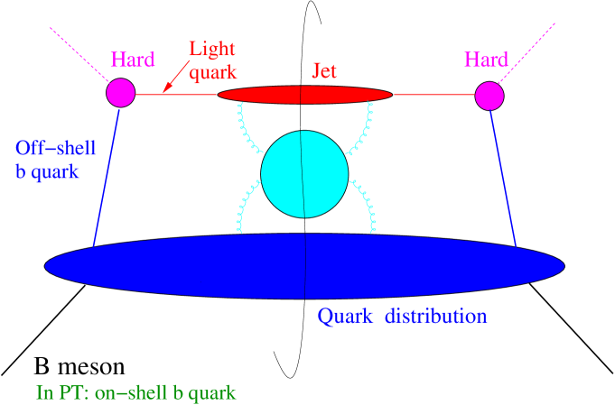
Figure 1: Factorization of inclusive decays into “hard”, “jet” and “soft” functions, with virtualities of order $m_{b}$, $m_{b}/\sqrt{N}$ and $m_{b}/N$, respectively. The jet function describes an unresolved jet with a given mass; see Ref. GR and Sec. III below. In inclusive decays the “soft” function $S_{N}(m_{b};\mu_{F})$ has the process–independent interpretation of a quark distribution function. This function describes the longitudinal momentum distribution of an off-shell b quark field in the initial state (an on-shell b quark in perturbation theory, and a ${\bar{B}}$ meson in the full theory). See Ref. QD for a precise definition.

Sudakov logarithms, reflecting the hierarchy $Q/N\,\ll\,Q/\sqrt{N}\,\ll\,Q$, can be resummed to all orders. One expects, however, that a purely perturbative treatment will only be valid for $Q/N\gg\Lambda$. Even then, extremely soft gluons with virtualities ${\cal O}(\Lambda)$, whose interaction is not described by perturbation theory, have some effect on the distribution. These gluons become increasingly important as the hierarchy $Q/N\gg\Lambda$ is removed. Considering the large–$N$ limit for fixed $Q$, one finds that the threshold region is characterized not only by Sudakov logarithms but also by non-perturbative effects that are inversely proportional to the “soft scale”, powers of $N\Lambda/Q$, which eventually always get larger than the logarithms as $N$ increases.

Importantly, the perturbative calculation itself reflects the presence of parametrically–enhanced power corrections: the series in the exponent of Eq. (5) is non-summable owing to infrared renormalons DGE_thrust ; Gardi:2001di . In conventional Sudakov resummation this infrared sensitivity is ignored: the perturbative sum is truncated, not regularized. A regularization is necessary in order to systematically separate between logarithmically–enhanced perturbative corrections and power–enhanced non-perturbative power corrections. Such power corrections are uniquely associated with the phase–space region from which the logarithms arise, and therefore their physical interpretation is straightforward. For example, in event–shape distribution the all–order resummation of (large–angle) soft gluon emission exposes parametrically–enhanced hadronization corrections; in inclusive decay spectra (Fig. 1) all–order soft–gluon resummation exposes parametrically–enhanced corrections distinguishing the quark distribution in the initial–state meson from that in an on-shell heavy quark.

The presence of infrared renormalons and parametrically–enhanced power corrections in the moment–space Sudakov factor is completely general, and it has far–reaching implications for the analysis of inclusive distributions. On general grounds, independently of the renormalon perspective, treatment of power corrections on the soft scale for $N\sim Q/\Lambda$ requires the introduction of a new non-perturbative function Neubert:1993um ; Neubert:1993ch ; Bigi:1993ex ; Korchemsky:1999kt , the so-called “shape function”. Unfortunately, the “shape function” is hard to constrain theoretically, while if constrained by data alone the result would strongly depend on the functional form assumed and on the perturbative approximation with which it is combined.

In practice, the threshold region was addressed by different tools in different applications, usually introducing some infrared cutoff on the perturbative result and parametrizing the contributions from the infrared as a “shape function”. Having little theoretical constraints on this function, the predictive power has been, in general, very limited. The most familiar examples are:

• Event–shape distributions: Hadronization effects are taken into account though a leading non-perturbative “shift” of the Sudakov resummed spectrum Dasgupta:2003iq ; Dokshitzer:1997ew ; Korchemsky:1995zm or, when addressing the peak region, through a convolution with a “shape function” Korchemsky:1999kt ; Korchemsky:2000kp . The general strategy of quantifying hadronization effects by power corrections represents an important advancement with respect to their description through fragmentation models in event generators. This approach quickly led to successful phenomenology for average values of event shapes Korchemsky:1995zm –Milan , Gardi:1999dq , but the challenge of describing the spectrum in the peak region could not easily be met.

• Heavy–meson production cross sections: Fragmentation of the heavy quark into a meson is taken into account through a convolution with a leading–power fragmentation function Kart ; Peterson . Applied with or without Sudakov resummation, usually without any momentum cutoff, see e.g. Cacciari:2005uk .

• Inclusive B decay: The momentum distribution of the b quark in the B meson is taken into account through a convolution with a leading–power “shape function” Neubert:1993um ; Neubert:1993ch ; Bigi:1993ex ; Bosch:2004th ; Lange:2005yw . Applied with or without Sudakov resummation, using a momentum cutoff.

Major progress in addressing this problem from first principals was made in recent years by Dressed Gluon Exponentiation (DGE). In DGE the moment–space Sudakov exponent is computed as an all–order Borel sum, avoiding the usual logarithmic–accuracy truncation. Power–like separation between perturbative and non-perturbative corrections on the “soft scale” $Q/N$ is achieved by the Principal Value prescription, avoiding any arbitrary momentum cutoff. This opens the way for making full use of the inherent infrared safety of the observable, which often extends beyond the logarithmic level. Infrared factorization and renormalization–group invariance strongly constrain the universal, all–order structure of the exponent. Additional, observable–dependent properties are derived from renormalon calculations of the corresponding Sudakov anomalous dimensions. These translate into constraints on the parametric form of power corrections that affect the exponentiation kernel. The end result is that the physical spectrum can be approximated by the regularized perturbative DGE spectrum, supplemented by a few power corrections of a known parametric form. This highly predictive framework has led to successful phenomenology in a variety of applications, including in particular event–shape distributions DGE_thrust ; Gardi:2002bg , heavy–quark fragmentation CG and inclusive B decay spectra Andersen:2005bj ; Andersen:2005mj .

Our purpose here is to review the DGE approach from a general perspective. We will discuss the applications mainly to illustrate how the method works and distinguish between general and process–specific properties. We start, however, in Sec. II by shortly describing the motivation and the present status of the calculation of inclusive B decay spectra, where the application of DGE has proven useful for the interpretation of data from the B factories  BDK ; Andersen:2005bj ; Gardi:2005mf ; Andersen:2005mj ; Gardi:2006gt . In Sec. III we explain the foundation of the DGE approach using the example of an unresolved jet. This analysis GR is directly relevant for the problem of deep inelastic structure functions at large Bjorken $x$, where the power corrections can also be viewed as resummation of the Operator Product Expansion (OPE) Gardi:2002bk . Next, in Sec. IV, we turn to discuss large–angle soft radiation. We explain how constraints on power corrections follow from the properties of the corresponding Sudakov anomalous dimension. The success of the resulting power–correction phenomenology is demonstrated using examples from event–shape distributions, heavy–quark fragmentation and B decay spectra. This is followed by a short summary of our conclusions in Sec. V.

II Inclusive B decay spectra

Amongst the most important contributions of the B factories are inclusive B decay measurements Barberio:2006bi ; HFAG :

• inclusive semileptonic decays, which provide the most accurate way to determine the CKM parameters $|V_{\rm cb}|$ and $|V_{\rm ub}|$. The ratio $|V_{\rm ub}/V_{\rm cb}|$ is one of the important constraints on the unitarity triangle Bona:2005vz ; Charles:2004jd . It is also an essential input in probing new physics, for example through $B^{0}$–$\bar{B}^{0}$ mixing, see e.g. Ball:2006xx .

• inclusive radiative decay, ${\bar{B}}\longrightarrow X_{s}\gamma$, that directly probes the short–distance interaction responsible for flavor changing neutral currents. This decay, which occurs only through loops within the Standard Model, provides an important constraint on possible new physics scenarios Allanach:2006jc ; Gambino:2005dp .

Inclusive decays are theoretically favorable over exclusive ones owing to their low sensitivity to the hadronic structure of the initial and final states.

Owing to irreducible backgrounds, experimental measurements of inclusive decays are limited to certain kinematic regions. This makes the theoretical calculation of inclusive decay spectra an essential ingredient on the way from the measurement to its interpretation. This is the case for both the radiative and the charmless semileptonic decays; the exception is ${\bar{B}}\longrightarrow X_{c}l\bar{\nu}$ that can be measured over the whole kinematic range. In ${\bar{B}}\longrightarrow X_{s}\gamma$, only hard photons with $E_{\gamma}>1.8$ GeV, corresponding to $M_{X}\equiv\sqrt{(P_{B}-q)^{2}}=\sqrt{M_{B}(M_{B}-2E_{\gamma})}\mathrel{\mathchoice{\vbox{\offinterlineskip\halign{$\m@th\displaystyle\hfil#\hfil$\cr<\crcr\sim\crcr} }}{\vbox{\offinterlineskip\halign{$\m@th\textstyle\hfil#\hfil$\cr<\crcr\sim\crcr} }}{\vbox{\offinterlineskip\halign{$\m@th\scriptstyle\hfil#\hfil$\cr<\crcr\sim\crcr} }}{\vbox{\offinterlineskip\halign{$\m@th\scriptscriptstyle\hfil#\hfil$\cr<\crcr\sim\crcr} }}}3$ GeV, can be distinguished from the background; the measurement becomes statistically limited only for $E_{\gamma}\mathrel{\mathchoice{\vbox{\offinterlineskip\halign{$\m@th\displaystyle\hfil#\hfil$\cr>\crcr\sim\crcr} }}{\vbox{\offinterlineskip\halign{$\m@th\textstyle\hfil#\hfil$\cr>\crcr\sim\crcr} }}{\vbox{\offinterlineskip\halign{$\m@th\scriptstyle\hfil#\hfil$\cr>\crcr\sim\crcr} }}{\vbox{\offinterlineskip\halign{$\m@th\scriptscriptstyle\hfil#\hfil$\cr>\crcr\sim\crcr} }}}2.1$ GeV. For the charmless semileptonic decay, ${\bar{B}}\longrightarrow X_{u}l\bar{\nu}$, the situation is yet more difficult: an upper cut on the hadronic invariant mass $M_{X}<1.7$ GeV must be applied to avoid the overwhelming charm background. Thus, the determination of $|V_{\rm ub}|$ from inclusive measurements strongly relies on the theoretical calculation of the spectrum.

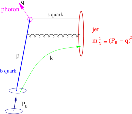
Figure 2: The kinematics in ${\bar{B}}\longrightarrow X_{s}\gamma$: the photon, carrying momentum $q$ (with $q^{2}=0$), recoils against the hadronic jet. In general, the virtuality of the b quark when decaying is a consequence of its “primordial” Fermi motion as well as of its subsequent interaction. In the on-shell approximation, where perturbation theory applies, the “primordial” Fermi motion, namely the interaction of the b quark with the light degrees of freedom in the meson is neglected; then the $b$ quark momentum in the meson rest frame is $p=(m_{b},\vec{0})$ while the momentum of the light degrees of freedom is $k=(\bar{\Lambda},\vec{0})$, with $\bar{\Lambda}=M_{B}-m_{b}$, where $M_{B}$ is the meson mass and $m_{b}$ is the quark pole mass.

As dictated by the Born–level process, the typical hadronic momentum configuration in heavy–to–light decays is jet–like (see Fig. 2): in the B rest frame the hadronic system has a high energy and a small mass, $M_{X}\ll M_{B}$. The spectra peak near threshold, making the understanding of this limit absolutely essential. As discussed above, only the small–$M_{X}$ region is experimentally accessible.

An important observation underlying the theoretical description of inclusive heavy–to–light decay spectra, is that the decaying b quark is not on-shell Neubert:1993um ; Neubert:1993ch ; Bigi:1993ex . The Fermi motion of the b quark in the meson involves momenta of ${\cal O}(\Lambda)$, and therefore one can expect ${\cal O}(\Lambda)$ smearing of the perturbative spectrum by non-perturbative effects. The common lore, which developed based on this physical picture, is that computing the spectrum in the peak region is strictly beyond the limits of perturbative QCD.

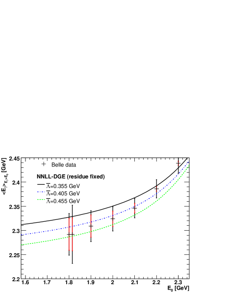
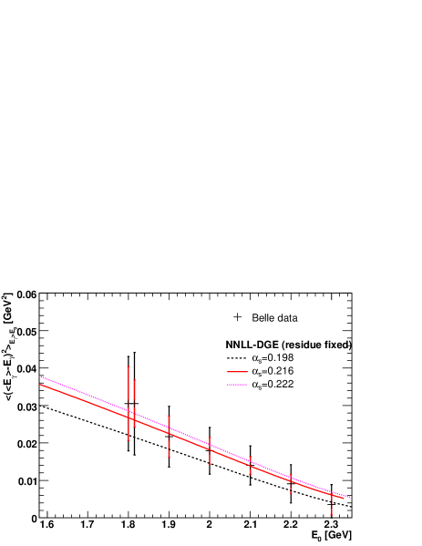
Figure 3: $\bar{B}\longrightarrow X_{s}\gamma$ theory vs. data: The average energy (left) and the variance (right) with a cut $E_{\gamma}>E_{0}$, as calculated by DGE in Andersen:2005bj in the on-shell approximation (i.e. with no power corrections), varying the short distance parameters $m_{b}^{\hbox{\tiny${\overline{\rm MS}}$}}$ and $\alpha_{s}^{\hbox{\tiny${\overline{\rm MS}}$}}$ within their error range. The result is compared with data from Belle Belle05 . Inner and total error bars show systematic and statistical plus systematic errors (added in quadrature), respectively.

In fact, the situation is significantly better Andersen:2005bj ; Gardi:2005mf ; Andersen:2005mj ; Gardi:2006gt : a systematic on-shell calculation involving resummation of the perturbative expansion yields a good approximation to the meson decay spectrum, one which provides an excellent starting point for quantifying non-perturbative corrections.

The on-shell approximation is physically natural because the heavy quark carries most of the momentum of the meson: the b quark virtuality, ${\cal O}(\Lambda)$, is much smaller than the mass. When considering the total rate this translates into a systematic expansion in inverse powers of the mass, where the leading corrections are ${\cal O}(\Lambda^{2}/m_{b}^{2})$ and are numerically small.

The next, crucial observation is that the on-shell decay spectrum is infrared and collinear safe, namely all its moments have finite coefficients to any order in perturbation theory. This means that non-perturbative effects, which make for the difference between the on-shell approximation and the physical meson decay, appear in moment space only through power corrections. Of course, when referring to the on-shell decay spectrum one must address the question of the summability of the expansion (as well as the precise definition of the on-shell mass), which brings about the issue of infrared renormalons.

In general, the virtuality of the decaying b quark is a consequence of its “primordial” Fermi motion and of its subsequent interaction. This, however, does not preclude the resummed on-shell spectrum being a good approximation to the meson decay spectrum. Obviously, the “primordial” Fermi motion and the “subsequent interaction” need to be defined. This definition amounts to a separation between non-perturbative and perturbative contributions, which can be done in a variety of ways. Cutoff–based separation procedures Neubert:1993um –Lange:2005yw , Bigi:1996si that are often applied, hinder the possibility of using of the inherent infrared safety of the on-shell decay spectrum. They necessarily associate a significant contribution with the non-perturbative “primordial” Fermi motion, which must be parametrized in a so-called “shape function”. Having little theoretical guidance, this parametrization is rather arbitrary, and the predictive power is very limited. The alternative used in DGE is separation at the level of powers, which is implemented using Principal Value Borel summation. In this way one can make full use of the inherent infrared safety of the on-shell decay spectrum, leaving only genuinely non-perturbative contributions, which distinguish between the (properly regularized) quark distribution in an on-shell quark and that in a meson, to be parametrized. Moreover, this parametrization is well guided by the theory: a small number of non-perturbative power corrections of a known form (see below) would suffice. In fact, with present experimental data no power corrections are needed — see Fig. 3.

It must be emphasized that the on-shell decay spectrum can only be an approximation to the physical spectrum when considered to all orders. In particular, both the on-shell mass, which sets the perturbative endpoint at any order in perturbation theory $E_{\gamma}\longrightarrow m_{b}/2$, or $x\equiv 2E_{\gamma}/m_{b}\longrightarrow 1$, and the spectral moments defined with respect to $x$ as in Eq. (3), have a leading infrared renormalon at $u=\frac{1}{2}$. The corresponding ambiguity cancels upon computing the sum of the series for $m_{b}$ and for the Sudakov factor using a systematic regularization — see Eq. (30) below. Examining the real–emission contribution to the spectrum in fixed–order perturbation theory (Fig. 4) one indeed observes huge corrections going from order to order. Considering the resummed spectrum by DGE, matched to NLO and NNLO, respectively Andersen:2005bj ; Andersen_Gardi_to_appear , one finds instead a remarkable stability, reflecting the fact that the dominant corrections have been resummed. Another striking difference between the resummed spectrum and the fixed–order one is their different support properties: the fixed–order result is a distribution that has support for $E_{\gamma}\leq m_{b}/2$, while the resummed result is a function that has support for $E_{\gamma}\leq(m_{b}+{\cal O}(\Lambda))/2\simeq M_{B}/2$, i.e. close to the physical spectrum. Evidently, resummation makes a qualitative difference.

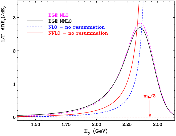
Figure 4: The $\bar{B}\longrightarrow X_{s}\gamma$ photon–energy spectrum (corresponding to the electromagnetic dipole operator $O_{7}$) in the on-shell approximation as computed in fixed–order perturbation theory at NLO and at NNLO, and by resummed perturbation theory (DGE) Andersen:2005bj ; Andersen_Gardi_to_appear , matched to NLO and NNLO, respectively. A common value of the (Principal Value) pole mass, $m_{b}=4.88\pm 0.05$ GeV, has been used. This value was computed Andersen:2005bj based on the measured short–distance quark mass in $\overline{\rm MS}$, $m_{b}^{\hbox{\tiny${\overline{\rm MS}}$}}=4.20\pm 0.04$ GeV Buchmuller:2005zv .

The ultimate test of the theoretical predictions is of course the comparison with experimental data. In $\bar{B}\longrightarrow X_{s}\gamma$ spectral data from Babar and Belle has become available shortly after the publication of the theocratical predictions by DGE Andersen:2005bj . Comparison of the first two spectral moments, computed with a varying lower cut $E_{\gamma}>E_{0}$, with Belle data is shown in Fig. 3; a similar comparison with BaBar data can be found in Ref. Gardi:2005mf . These results show that the resummed on-shell decay spectrum indeed provides a good approximation to the meson decay spectrum, as anticipated in Ref. Andersen:2005bj . Comparison of the computed $\bar{B}\longrightarrow X_{s}\gamma$ spectrum with data has several immediate applications:

• Extrapolation of the partial width from the region of measurement to the whole of phase space, in order to confront it with the Standard Model prediction and provide constrains on physics beyond the Standard Model.

• Precise determination of the b quark mass, see Ref. HFAG .

• Determination of the leading power corrections, the ones associated with the quark distribution in the meson. With the present accuracy, power corrections cannot be determined, but higher precision data are expected in the near future. Owing to their universality, these power corrections can readily be used in improving theoretical predictions for other inclusive decay spectra, notably the charmless semileptonic spectrum.

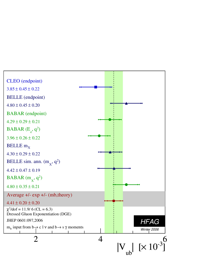
Figure 5: $|V_{\rm ub}|$ as extracted using DGE Andersen:2005mj by the Heavy Flavor Averaging Group (HFAG) HFAG from inclusive semileptonic measurements by CLEO, Belle and BaBar.

A pressing issue, which is high on the agenda of the B factories is the precise determination of $|V_{\rm ub}|$. As mentioned above, inclusive measurements of charmless semileptonic decays provide the most promising avenue for this determination. The main obstacle is the large extrapolation from the region of measurement to the whole of phase space, which strongly relies on theoretical predictions for the spectrum. The strategy applied so far Barberio:2006bi made direct use of the universality of the quark distribution in the meson, by first fitting an ansatz for the “shape function” to the $\bar{B}\longrightarrow X_{s}\gamma$ decay data and then using it when computing the partial branching fraction of $\bar{B}\longrightarrow X_{u}l\bar{\nu}$ within the region of measurement. As discussed above, in this approach there is little theoretical guidance on the functional form of the “shape function”. Here the alternative presented by DGE is very attractive Andersen:2005mj ; Gardi:2006gt : in this framework the on-shell calculation, which depends only on the short–distance parameters, provides a good approximation to the spectrum. Moreover, prospects are high for improving this prediction further by higher–order (NNLO) calculations and by parametrization of the first few power corrections whose $N$–dependence is known.

The Heavy Flavor Averaging Group (HFAG) HFAG has recently performed a first comprehensive study of $|V_{\rm ub}|$ from inclusive decay measurements using DGE. This analysis, which is summarized in Fig. 5, provides the most precise determination of $|V_{\rm ub}|$ so far. Since different measurements in Fig. 5 correspond to different kinematic cuts with extrapolation factors ranging between $\sim 2$ and $5$, the consistency of the resulting values for $|V_{\rm ub}|$ provides an additional evidence that the underlying description of the spectrum is good. Direct comparison of the DGE calculation of the triple differential $\bar{B}\longrightarrow X_{u}l\bar{\nu}$ spectrum Andersen:2005mj (or its moments with varying cuts) with experimental data would be useful to constrain power corrections. Such analysis is complementary to the $\bar{B}\longrightarrow X_{s}\gamma$ one in several ways owing to the potential Weak Annihilation contributions and the different (non-universal) subleading power corrections in the two processes Bauer:2002yu –Lee:2004ja , effects that are hard to quantify theoretically and that have so far been neglected.

Having seen the advancement achieved by DGE in the calculation of inclusive decay spectra, let us now return to the theoretical foundation of the approach. Infrared and collinear safe observables, such as inclusive decay spectra or event–shape distributions, typically involve two distinct sources of large corrections, the jet function and the soft function in Eq. (7). We begin in Sec. III by considering the example of the jet function $J_{N}(Q,\mu_{F})$, which is common to a large class of inclusive cross sections and decay spectra Gardi:2001di ; CG ; BDK . In Sec. IV we turn to the soft function $S_{N}(Q,\mu_{F})$.

III An unresolved jet and deep inelastic structure functions near the elastic limit

Sudakov resummation is a manifestation of the infrared safety of inclusive distributions at the logarithmic level. However, the Sudakov evolution kernel conceals infrared sensitivity at the power level, which only becomes explicit once running–coupling effects are resummed to all orders. Consequently, Sudakov resummation involves power corrections that exponentiate along with the logarithms.

To demonstrate this, consider first the jet function Sterman:1986aj ; CT $J_{N}(Q;\mu_{F})$ that can be defined in a process independent way as the quark propagator in axial gauge (Eq. (2) in GR ). It obeys the following evolution equation:

$$\frac{d\ln J_{N}(Q;\mu_{F})}{d\ln Q^{2}}=\int_{0}^{1}dx\frac{x^{N-1}-1}{1-x}{\cal J}\left(\alpha_{s}((1-x)Q^{2})\right).$$ (8)

${\cal J}\left(\alpha_{s}\right)$ is the corresponding scheme–invariant anomalous dimension. It is usually decomposed in the ${\overline{\rm MS}}$ scheme as GR

$${\cal J}\left(\alpha_{s}(\mu^{2})\right)={\cal A}\left(\alpha_{s}(\mu^{2})\right)+\frac{d\alpha_{s}(\mu^{2})}{\ln\mu^{2}}\frac{d{\cal B}\left(\alpha_{s}(\mu^{2})\right)}{d\alpha_{s}}=C_{F}\frac{\alpha_{s}(\mu^{2})}{\pi}+\ldots,$$ (9)

where the conformal part, ${\cal A}\left(\alpha_{s}\right)$, is the universal cusp anomalous dimension, which is the coefficient of the singular part, $1/(1-x)_{+}$, in the splitting function Korchemsky:1988si . ${\cal A}$ alone controls the factorization scale dependence of the jet function:

$$\frac{d\ln J_{N}(Q;\mu_{F})}{d\ln\mu_{F}^{2}}={\cal A}\left(\alpha_{s}(\mu_{F}^{2})\right)\ln N.$$ (10)

The anomalous dimension ${\cal B}(\alpha_{s})=-\frac{3}{4}\frac{\alpha_{s}}{\pi}+\ldots$ is associated with collinear singularities Sterman:1986aj ; CT in the axial–gauge light–quark propagator, and its perturbative expansion is currently known to NNLO MVV ; Moch:2005ba .

The jet function $J_{N}(Q;\mu_{F})$ is also the Sudakov factor controlling the $x\longrightarrow 1$ limit of deep inelastic structure functions GR ,

$$F_{2}^{N}(Q^{2})\equiv\int_{0}^{1}dxx^{N-2}F_{2}(x,Q^{2})\simeq\underbrace{\Big{[}H(Q;\mu_{F})\,J_{N}(Q;\mu_{F})\,+\,{\cal O}(1/N)\Big{]}}_{\rm twist-two\,\,coefficient\,\,function}\,\times\,q_{N}(\mu_{F})\,+\,{\cal O}(N\Lambda^{2}/Q^{2}),$$ (11)

where $q_{N}(\mu_{F})$ is the quark distribution function, and $H(Q;\mu_{F})$ is a hard function that does not depend on $N$. The evolution of the quark distribution function $q_{N}(\mu_{F})$ is controlled at large $N$ by the cusp anomalous dimension ${\cal A}\left(\alpha_{s}\right)$:

$$\frac{d\ln q_{N}(\mu_{F})}{d\ln\mu_{F}^{2}}=-{\cal A}\left(\alpha_{s}(\mu_{F}^{2})\right)\ln N\,+\,{\cal O}(1)$$ (12)

such that the product in Eq. (11) is invariant.

The evolution equation of the structure function itself (at leading twist) is

$$\frac{d\ln F_{2}^{N}(Q^{2})}{d\ln Q^{2}} = \frac{d\ln J_{N}(Q;\mu_{F})}{d\ln Q^{2}}+\frac{d\ln H(Q;\mu_{F})}{d\ln Q^{2}}+{\cal O}(1/N)$$

$$= \int_{0}^{1}dx\frac{x^{N-1}-1}{1-x}{\cal J}\left(\alpha_{s}((1-x)Q^{2})\right)+\frac{d\ln H(Q;\mu_{F})}{d\ln Q^{2}}+{\cal O}(1/N),$$

implying that log–enhanced terms in the leading–twist coefficient function of $F_{2}$ exponentiate in moment space, to any order in perturbation theory.

The cancellation between real $(x^{N-1})$ and virtual $(-1)$ contributions guaranties that the evolution kernel on the r.h.s of Eq. (III) or Eq. (8) is finite at any order in perturbation theory, despite the $1/(1-x)$ singularity. Given that the anomalous dimension ${\cal J}\left(\alpha_{s}(\mu^{2})\right)$ is known to a certain order (currently NNLO MVV , with a good estimate of the N³LO Moch:2005ba ) one can use the $\beta$ function and integrate the r.h.s of Eq. (8) order by order, obtaining the following expansion:

$${\rm r.h.s\,\Big{\{}Eq.~{}(\ref{J_ev})\Big{\}}}\,=\,C_{F}\,\sum_{j=1}^{\infty}\sum_{l=1}^{j}c_{j,l}\,\left(\frac{\alpha_{s}(Q^{2})}{\pi}\right)^{j}(\ln N)^{l},$$ (14)

where the coefficients $c_{j,l}$ with $l=j$ at any order $j$ (leading logarithms, LL) are determined by the LO term in ${\cal J}\left(\alpha_{s}\right)$, those with $l=j-1$ (next–to–leading logarithms, NLL) require also the NLO term in ${\cal J}\left(\alpha_{s}\right)$, etc. The standard approach to Sudakov resummation is based on expressing the sum in Eq. (14) as an expansion with increasing logarithmic accuracy, namely

$${\rm r.h.s\,\Big{\{}Eq.~{}(\ref{J_ev})\Big{\}}}\,=\,\frac{C_{F}}{\beta_{0}}\,\sum_{n=0}^{\infty}g_{n}(\lambda)\left(\frac{\alpha_{s}(Q^{2})}{\pi}\right)^{n}\,;\qquad\quad\lambda\equiv\frac{\beta_{0}\alpha_{s}(Q^{2})}{\pi}\,\ln N,$$ (15)

where $\beta_{0}=\frac{11}{12}C_{A}-\frac{1}{6}N_{f}$. Here $g_{0}(\lambda)=\ln(1-\lambda)$, and higher–order terms $g_{n}(\lambda)$ are determined based on the expansion of ${\cal J}\left(\alpha_{s}\right)$ to NⁿLO. This sum is therefore truncated at $n=n_{\max}$, the order at which ${\cal J}\left(\alpha_{s}\right)$ has been computed.

The next, crucial observation DGE_thrust ; Gardi:2001di ; GR is that the sum in Eq. (15) does not converge. The same is true for any reorganization of the terms in Eq. (14) because the coefficients $c_{j,l}$ increase as $j!$ at high orders. This is the effect of an infrared renormalon that dominates the evolution kernel in Eq. (8) at high orders. Importantly, ${\cal J}$, being an anomalous dimension, is expected to be free of any renormalon singularities. Thus, the one and only source of factorial divergence in Eq. (8) is the integration over the momentum fraction $x$ near $x\longrightarrow 1$. In this limit the coupling in ${\cal J}\left(\alpha_{s}(\mu^{2})\right)$ is probed at extremely soft momentum scales $\mu^{2}\longrightarrow 0$. The non-existence of the sum in Eqs. (15) or (14) reflects sensitivity to the far infrared at the power level.

A systematic way to quantify this infrared sensitivity is to regularize the divergence as a Borel sum. To this end, imagine that the anomalous dimension ${\cal J}\left(\alpha_{s}\right)$ on the r.h.s. of Eq. (8) were known to all orders, so one could write its scheme–invariant Borel representation:

$${\cal J}\left(\alpha_{s}(\mu^{2})\right)=\frac{C_{F}}{\beta_{0}}\int_{0}^{\infty}du\left(\frac{\Lambda^{2}}{\mu^{2}}\right)^{u}T(u)\,B_{\cal J}(u),$$ (16)

where $T(u)$ is the Borel transform of the coupling. Using Eq. (16) in Eq. (8) (or in Eq. (III)) one can perform the $x$ integration arriving at:

$$\frac{d\ln J_{N}(Q;\mu_{F})}{d\ln Q^{2}}=\frac{C_{F}}{\beta_{0}}\int_{0}^{\infty}du\left(\frac{\Lambda^{2}}{Q^{2}}\right)^{u}T(u)\,B_{\cal J}(u)\,\left[\frac{\Gamma(N)\Gamma(-u)}{\Gamma(N-u)}+\frac{1}{u}\right].$$ (17)

Indeed, one finds potential renormalon ambiguities at positive integer values of $u$ arising from the $x\longrightarrow 1$ limit. As mentioned above, $B_{\cal J}(u)$ is not expected to have any renormalon singularities, however, unless it vanishes at $u=k$ where $k=1,2,\ldots$, the evolution kernel (the r.h.s. of Eq. (17)) will have power-like ambiguities that scale at large $N$ as $(N\Lambda^{2}/Q^{2})^{k}$. Upon solving the evolution equation for $J_{N}(Q;\mu_{F})$, any such power terms would obviously exponentiate along with the logarithms.

The discussion of renormalons can be made concrete by focusing on the gauge–invariant set of radiative corrections corresponding to the large–$\beta_{0}$ limit. In this limit one can get analytic results for the Borel transform. The result for the anomalous dimension reads GR :

$$B_{\cal J}(u)\bigg{|}_{{\rm large}\,\beta_{0}}=\,\frac{{\rm e}^{\frac{5}{3}u}}{2}\,\frac{\sin\pi u}{\pi u}\,\left(\frac{1}{1-u}+\frac{1}{1-u/2}\right),$$ (18)

implying that renormalon singularities in Eq. (17) at $u=1$ and $u=2$ are indeed present. Consequently, Sudakov resummation cannot be considered a purely perturbative issue: the evolution kernel itself is only defined in perturbation theory up to powers. Since the l.h.s of Eq. (III) is an observable, these ambiguities must cancel once non-perturbative effects are systematically included. Indeed, within the OPE renormalon ambiguities reflect the mixing under renormalization between operators of different twist Beneke:1998ui ; Gardi:2002bk ; Braun:2004bu ; in the case of $F_{2}$ this issue is understood in full detail at twist four, see Ref. Gardi:2002bk . Of course, the OPE cannot be directly applied to the evolution equation (17), which was only derived at the leading–twist level. The exponentiation of these power corrections Gardi:2002bk ; GR goes beyond the OPE analysis: it amounts to resumming the OPE.

Importantly, $B_{\cal J}(u)$ in Eq. (18) vanishes at certain integer values $u=k$, for $k\geq 3$, so the corresponding renormalon ambiguities in the evolution kernel (17) are absent. Since a single dressed gluon is a natural approximation to the evolution kernel (e.g. iteration of a single chain is generated by solving the equation, through exponentiation) we expect that the pattern of renormalon singularities exposed in the large–$\beta_{0}$ limit would not be modified. We will therefore assume that the zeros of $B_{\cal J}(u)$ in Eq. (18) are the zeros of this function in the full theory. As we shall see in the next section, other Sudakov anomalous dimensions are characterized by their own pattern of zeros.

In general, Borel singularities in QCD differ from their large–$\beta_{0}$ limit in both the value of the residue and the nature of the singularity Mueller:1984vh ; Beneke:1998ui . However, Borel singularities in the Sudakov evolution kernel remain simple poles GR . This follows directly from Eq. (17) and the above conjecture that $B_{\cal J}(u)$ itself does not have Borel singularities.

To make practical use of Eq. (17) one obviously needs sufficient knowledge of the Borel transform of the Sudakov anomalous dimension, $B_{\cal J}(u)$. Perturbation theory directly gives the Taylor expansion of $B_{\cal J}(u)$ near the origin. Examining the integral in Eq. (17) one finds that at small $N$ only the immediate vicinity of the origin is relevant, while for $N\sim{\cal O}(Q^{2}/\Lambda^{2})$ contributions from $u\sim 1$ and $u\sim 2$ become important. Owing to the strong suppression of contributions from large $u$ through $\Gamma(-u)$, the behavior of $B_{\cal J}(u)$ at large $u$ is irrelevant, even for high moments. Aiming at power accuracy, one would need to have $B_{\cal J}(u)$ under control at least for $0\leq u\mathrel{\mathchoice{\vbox{\offinterlineskip\halign{$\m@th\displaystyle\hfil#\hfil$\cr<\crcr\sim\crcr} }}{\vbox{\offinterlineskip\halign{$\m@th\textstyle\hfil#\hfil$\cr<\crcr\sim\crcr} }}{\vbox{\offinterlineskip\halign{$\m@th\scriptstyle\hfil#\hfil$\cr<\crcr\sim\crcr} }}{\vbox{\offinterlineskip\halign{$\m@th\scriptscriptstyle\hfil#\hfil$\cr<\crcr\sim\crcr} }}}1$, and specifically, constrain the value of $B_{\cal J}(u=1)$ that controls the magnitude of the leading renormalon residue in the evolution kernel.

It is natural to express $B_{\cal J}(u)$ in terms of its known large–$\beta_{0}$ limit as follows:

$$B_{\cal J}(u)=\left.B_{\cal J}(u)\right|_{{\rm large}\,\beta_{0}}\times V_{\cal J}(u)\,;\qquad\qquad V_{\cal J}(u)=1+{\cal O}(u/\beta_{0}),$$ (19)

where $V_{\cal J}(u)$ accounts for contributions that are subleading for $\beta_{0}\longrightarrow\infty$; its Taylor expansion around $u=0$ can be determined order by order in perturbation theory. Eq. (19) is consistent with $B_{\cal J}(u)$ having the same pattern of zeros as exposed by the large–$\beta_{0}$ limit (18) provided that $V_{\cal J}(u)$ itself has no singularities nor zeros, at least for positive integer values of $u$. A concrete ansatz that satisfies these requirements is $V_{\cal J}(u)=\exp(-w_{1}u-w_{2}u^{2}+\cdots)$. Here the coefficients $w_{i}$ are determined order by order, up to the order at which ${\cal J}(\alpha_{s})$ has been computed GR : based on the NLO result for the cusp anomalous dimension and Eq. (9) one finds $w_{1}=\frac{C_{A}}{\beta_{0}}\left(\frac{\pi^{2}}{12}-\frac{1}{3}\right)$, from the NNLO result for ${\cal J}(\alpha_{s})$ one can determine $w_{2}$, see Eq. (2.33) in Andersen:2005bj , and finally from the approximate Moch:2005ba N³LO coefficient for ${\cal J}(\alpha_{s})$ one can determine $w_{3}$ to good accuracy.

The characteristic feature of the power ambiguities of Eq. (17) is their enhancement by the moment index $N$, reflecting the fact that the physical scale involved is $Q^{2}/N$, the invariant mass of the jet. In the language of non-local lightcone operators BB , the large–$N$ limit corresponds to the limit of large lightcone separation between the quark fields Gardi:2002bk . Alternatively, within the local OPE this parametric enhancement is understood as power increase in the number of relevant local operators. This leads to an explosion in the number of non-perturbative parameters, making the description of structure functions in the large–$x$ limit within the framework of the OPE completely impractical.

Physically, the breakdown of the OPE and the appearance of non-perturbative corrections on the jet mass scale are related to the transition into the resonance region Liuti:2001qk ; Melnitchouk:2005zr , where eventually the jet becomes a few exclusive states. Obviously, the wealth of non-perturbative phenomenon in this region cannot be described in detail using the OPE. However, parton–hadron duality may well work in moment space up to very large $N$.

The discussion above suggests a clear track along which the evolution of structure functions at large–$x$ should be computed Gardi:2002bk ; GR :

• First, the evolution kernel on the r.h.s of Eq. (17) needs to be regularized, e.g. by taking the Principal Value of the Borel sum. Upon solving the evolution equation with the regularized kernel (and matching with the fixed–order result) one obtains an improved approximation to the evolution of the structure function at large $N$, which is valid up to ${\cal O}(N\Lambda^{2}/Q^{2})$ corrections.

• For sufficiently large $N$, the ${\cal O}(N\Lambda^{2}/Q^{2})$ power ambiguities become relevant, and the perturbative evolution should be supplemented by non-perturbative power corrections. Since power ambiguities appear in the evolution kernel, power corrections appear in the Sudakov exponent. The perturbative jet function is then modified by a multiplicative non-perturbative factor of a particular form that is dictated by the ambiguities,

  $$J_{N}(Q,\mu_{F})\,\longrightarrow\,J_{N}^{\rm PV}(Q,\mu_{F})\,\times\,J_{N}^{\rm NP(PV)}\left(Q\right);$$

  $${\rm where}\qquad J_{N}^{\rm NP(PV)}\left(Q\right)=\exp\Big{(}{-\omega_{1}^{\rm PV}(N-1)\left({\Lambda^{2}}/{Q^{2}}\right)-\omega_{2}^{\rm PV}(N-1)(N-2)\left({\Lambda^{2}}/{Q^{2}}\right)^{2}}\Big{)}.$$ (20)

  The non-perturbative parameters $\omega_{1,2}^{\rm PV}$ correspond to the regularization prescription (Principal Value) applied to the r.h.s of Eq. (17), such that the product $J_{N}^{\rm PV}(Q,\mu_{F})\,\times\,J_{N}^{\rm NP(PV)}(Q)$ is prescription–independent. It should be emphasized that by introducing power terms according to the ambiguity structure we explicitly assume a minimal model for the non-perturbative contribution: the first two power terms must definitely be there, but it is impossible to exclude by present theoretical tools higher power terms. To the extent that this assumption holds, Eq. (• ‣ III) sums up the dominant corrections in the OPE, scaling as powers of $N\Lambda^{2}/Q^{2}$, to all orders (cf. Eq. (11)) Gardi:2002bk :

  $$F_{2}^{N}(Q^{2})\,\simeq\,\Big{[}H(Q;\mu_{F})\,J_{N}^{\rm PV}(Q;\mu_{F})\,\times\,J_{N}^{\rm NP(PV)}\left(Q\right)\,+\,{\cal O}(1/N)\Big{]}\,\times\,q_{N}(\mu_{F})\,+\,{\cal O}(\Lambda^{2}/Q^{2}).$$ (21)

Ultimately, large–$x$ structure function data can be analyzed along these lines. Conventional structure function phenomenology Martin:2003sk (see, however, Refs. CM ; GR ; Yang:1999xg ; Alekhin:1998df ) does not focus on constraining high moments, and parton–distribution–function fits are typically done with a cut on the hadronic mass, $Q^{2}(1-x)/x>12.5\,{\rm GeV}^{2}$, restricting the data considered. In this way one avoids the need for Sudakov resummation or higher–twist corrections. Obviously, such restrictions limit the possibility of constraining the parton distribution functions. With the theoretical tools described above, there are high prospects for improving these constraints.

IV Soft gluons, Sudakov anomalous dimensions and parametrically–enhanced power corrections

In the previous section we discussed the DGE approach in the context of the exclusive limit of deep inelastic structure functions. This problem is special since it is characterized by a single hierarchy: the invariant mass of the jet $Q^{2}(1-x)/x$ gets significantly smaller than the hard momentum transfer $Q^{2}$; when the jet–mass scale approaches the hadronic scale, the structure function directly probes the exclusive limit, where the jet is composed of a few hadrons. As explained in the introduction, other inclusive distributions have a more complex structure, where the threshold region is characterized by a double hierarchy. Specifically, infrared and collinear safe observables such as event–shape distributions and inclusive decay spectra involve the following three scales: hard ${\cal O}(Q)$, “jet” ${\cal O}(Q/\sqrt{N})$ and “soft” ${\cal O}(Q/N)$. In this situation the threshold region, where Sudakov resummation is important, is parametrically wider than the exclusive region discussed above. Moreover, the most important power corrections are then the ones associated with large–angle soft emission, powers of $N\Lambda/Q$, whereas the non-perturbative structure of the jet, i.e. powers of $N\Lambda^{2}/Q^{2}$, can usually be neglected.

In this section we consider Sudakov factors associated with soft–gluon emission, which we denote in general by $S_{N}(Q;\mu_{F})$. The Sudakov factor $S_{N}(Q;\mu_{F})$ is defined at the level of the cross section so it involves the amplitude times the complex conjugate amplitude. Soft gluons do not resolve the hard interaction nor the structure of the jet; they couple to the color field along the classical trajectories of hard partons Gatheral:1983cz ; Frenkel:1984pz ; Sterman:1986aj . The relevant log–enhanced terms can therefore be computed in the Eikonal approximation or, equivalently, by considering Wilson–line operators KR87 ; Korchemsky:1991zp ; Korchemsky:1988si ; Korchemsky:1992xv ; Korchemskaya:1992je — see Fig. 6. Such field–theoretic definitions are useful because they readily generalize the perturbative Sudakov factor to the non-pertubative level Korchemsky:1992xv ; QD ; Korchemsky:1999kt .

“Soft” Sudakov factors corresponding to different observables are the same only in the conformal limit (or to leading logarithmic accuracy) where just the cusps along the Wilson loop contribute; subleaing logarithms and power corrections depend on the geometry of the process (Fig. 6) and on the way particle momenta are weighted. Indeed, already at the perturbative level $S_{N}(Q;\mu_{F})$ have different physical content in different processes, for example:

• In Drell–Yan or Higgs production near partonic threshold $S_{N}(Q;\mu_{F})$ describes the energy distribution of soft gluons ($1-x$ is the small energy fraction carried by gluons) emitted by the incoming partons, which can be represented in terms of lightlike Wilson lines CMW ; Contopanagos:1996nh ; Sterman:1986aj ; Collins:1984kg ; Korchemsky:1994is ; Beneke:1995pq ; Gardi:2001di ; Laenen:2000ij .

• In a large class of event–shape distributions in $e^{+}e^{-}$ annihilation DGE_thrust ; Gardi:2003iv ; Gardi:2002bg , $S_{N}(Q;\mu_{F})$ stands for the contribution to the observable by (large–angle) soft gluons that are emitted off the recoiling quark–antiquark in the two–jet limit. It can formally be described in terms of a weighted integral over a matrix element involving lightlike Wilson lines Korchemsky:1999kt ; Belitsky:2001ij .

• In heavy–quark fragmentation $S_{N}(m;\mu_{F})$ describes soft gluon radiation off an off–shell heavy quark that was initially produced with high energy of ${\cal O}(Q)$, where $Q\gg m$, and then gradually looses its energy approaching its mass shell. This radiation is dominated by transverse momenta (or virtualities) of order $|k_{\perp}|\sim m(1-x)$, — the “soft” scale — where $x$ is the longitudinal momentum fraction carried by the final–state on-shell heavy quark (which represents the detected heavy hadron on the perturbative level) DKT ; DKT95 ; CC ; CG ; Gardi:2003ar ; Melnikov:2004bm . The description of $S_{N}(m;\mu_{F})$ in terms of Wilson lines involves timelike lines connected by a finite lightlike segment of length $y^{-}$ that is proportional to $N$ Korchemsky:1992xv ; QD .

• In heavy–meson decay spectra $S_{N}(m;\mu_{F})$ describes the soft gluon interaction with the heavy quark prior to its decay. Formally, $S_{N}(m;\mu_{F})$ is the Sudakov factor associated with the longitudinal momentum distribution of an off-shell heavy–quark field in an on-shell heavy–quark initial state. Remarkably, it is identical to the Sudakov factor in heavy–quark fragmentation QD , while the non-perturbative dynamics in the two cases is different.

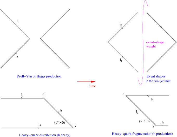
Figure 6: Representation of the soft Sudakov factor $S_{N}(Q;\mu_{F})$ in terms of Wilson–line operators in Minkowski space–time, where the time is the horizontal axis. The four diagrams correspond to Drell–Yan or Higgs production, event–shape distributions in the two–jet limit, heavy–quark distribution (inclusive decays), and heavy–quark fragmentation (heavy–meson production). In each case the lines close at infinity to form a loop, which guarantees gauge invariance.

Despite the different physics described by the “soft” Sudakov factor in different processes, $S_{N}(Q;\mu_{F})$ has a universal structure that is constrained by factorization, infrared safety and renormalization–group invariance. In particular, in all the examples mentioned above, upon neglecting ${\cal O}(1/N)$ corrections one can establish an evolution equation that is analogous to the jet–function case (8):

$$\frac{d\ln S_{N}(Q;\mu_{F})}{d\ln Q^{2}}\,=\,-\int_{0}^{1}dx\,\frac{x^{N-1}-1}{1-x}\,\,{\cal S}\left(\alpha_{s}((1-x)^{2}Q^{2})\right).$$ (22)

This equation implies exponentiation of all the logarithms to any order in perturbation theory. The observable–dependent, but scheme–invariant anomalous dimension ${\cal S}\left(\alpha_{s}\right)$ is usually decomposed in ${\overline{\rm MS}}$ as:

$${\cal S}\left(\alpha_{s}\right)={\cal A}\left(\alpha_{s}\right)\!+\!\frac{d\alpha_{s}}{\ln\mu^{2}}\frac{d{\cal D}\left(\alpha_{s}\right)}{d\alpha_{s}}=C_{F}\frac{\alpha_{s}}{\pi}+\ldots,$$ (23)

where ${\cal A}(\alpha_{s})$ is the universal cusp anomalous dimension appearing in Eq. (9) and ${\cal D}(\alpha_{s})$ is observable–dependent. The dependence of $S_{N}(Q;\mu_{F})$ on $\mu_{F}$ is the same as that of the $\overline{\rm MS}$ quark distribution, i.e. it has the opposite sign to Eq. (10) above, making the product in Eq. (7) factorization–scale invariant.

Similarly to the jet–function case, infrared sensitivity at power level is concealed in the r.h.s to the evolution equation (22): in the $x\longrightarrow 1$ limit the coupling is probed at extremely soft momentum scales, $\mu^{2}=Q^{2}(1-x)^{2}\longrightarrow 0$. In conventional Sudakov resummation this sensitivity is not regularized and the resulting divergent series is truncated at some order (some logarithmic accuracy). In order to regularize the divergence and quantify the infrared sensitivity as power–suppressed ambiguities we introduce a Borel representation for the anomalous dimension ${\cal S}\left(\alpha_{s}\right)$ in analogy with Eq. (16):

$${\cal S}\left(\alpha_{s}(\mu^{2})\right)=\frac{C_{F}}{\beta_{0}}\int_{0}^{\infty}du\left(\frac{\Lambda^{2}}{\mu^{2}}\right)^{u}T(u)B_{\cal S}(u).$$ (24)

Using (24) in (22), and performing the $x$ integration, one obtains the DGE form of the evolution equation:

$$\frac{d\ln S_{N}(Q;\mu_{F})}{d\ln Q^{2}}=-\frac{C_{F}}{\beta_{0}}\int_{0}^{\infty}du\left(\frac{\Lambda^{2}}{Q^{2}}\right)^{u}T(u)\times B_{\cal S}(u)\times\left[\frac{\Gamma(N)\Gamma(-2u)}{\Gamma(N-2u)}+\frac{1}{2u}\right].$$ (25)

Note that while Eq. (17) indicates potential renormalon singularities at all integer values of $u$, in Eq. (25) renormalons may occur also at half integer values. The corresponding power ambiguities at $u=\frac{k}{2}$ ($k$ being a positive integer) would scale at large $N$ as $(N\Lambda/Q)^{k}$. Specifically, the leading renormalon ambiguity can be at $u=\frac{1}{2}$, which would result in a substantial ${\cal O}(N\Lambda/Q)$ effect — a global shift of the distribution. Consequently, these power corrections received much attention in various applications including Drell–Yan production Korchemsky:1994is ; Beneke:1995pq ; Gardi:2001di (where the $u=\frac{1}{2}$ ambiguity was found not to occur, see below), heavy–quark fragmentation Nason:1996pk ; CG ; Gardi:2003ar and especially event–shape variables Korchemsky:1995zm –BM . Notably, the relevance of renormalons in computing inclusive B decay spectra has not received proper attention until recently BDK ; QD ; Andersen:2005bj ; Andersen:2005mj ; Gardi:2004gj ; Gardi:2005mf .

Since ${\cal S}\left(\alpha_{s}\right)$ is an anomalous dimension, $B_{\cal S}(u)$ is not expected to have any renormalon singularities of its own. It follows that the sole origin of renormalons in the evolution kernel is the integration over $x$ for $x\longrightarrow 1$, leading to simple poles in Eq. (25). As usual, perturbative QCD calculations facilitate the determination of the first few orders in ${\cal S}\left(\alpha_{s}\right)$, corresponding to the expansion of $B_{\cal S}(u)$ around the origin. In order to know the pattern of infrared renormalon singularities of the evolution kernel, one needs to know $B_{\cal S}(u)$ as an analytic function, and specifically find its zeros in order to deduce which power ambiguities are missing. Here the large–$\beta_{0}$ limit becomes useful: when considering the evolution kernel a single dressed gluon becomes a natural approximation; non-Abelian diagrams are expected to modify the residue of the renormalons by $C_{A}/\beta_{0}$–dependent contributions (${\cal O}(1)$ effects) but not to alter their positions. Thus, the pattern of zeros of $B_{\cal S}(u)$ can be directly deduced from the large–$\beta_{0}$ limit. Table 1 lists the results in some important examples. For each observable we quote the expression for $b_{\cal S}(u)$ that is related to the corresponding $B_{\cal S}(u)$ by:

$$B_{\cal S}(u)={\rm e}^{\frac{5}{3}u}\,\frac{\sin\pi u}{\pi u}\,b_{\cal S}(u)\,\times\,V_{\cal S}(u)\,;\qquad\quad V_{\cal S}(u)=1+{\cal O}(u/\beta_{0}),$$ (26)

where $V_{\cal S}(u)$ has no renormalon singularities nor zeros. The table also shows where, on the positive real axis, $\left.B_{\cal S}(u)\right|_{{\rm large}\,\beta_{0}}$ vanishes, thus eliminating the potential renormalon singularity on the r.h.s. of Eq. (25). Finally it shows which power ambiguities do appear. Evidently, the renormalon pattern is different for each class of distributions.

Table 1: Results for Sudakov anomalous dimensions in the large–$\beta_{0}$ limit, Eq. (26) DGE_thrust ; Gardi:2002bg ; Gardi:2001di ; CG ; GR ; Gardi:2003iv ; Beneke:1995pq ; QD , and the corresponding power corrections in the evolution kernel, the r.h.s of Eq. (25).

Observable	${\displaystyle b_{\cal S}(u)}$	$B_{\cal S}(u)=0$ for $u>0$	power corrections
Drell–Yan or Higgs production near partonic threshold	2${\displaystyle\frac{\Gamma^{2}(1-u)}{\Gamma(1-2u)}}$	$\displaystyle{u=\frac{1}{2},\frac{3}{2},\ldots}$	${\displaystyle\left(\frac{\Lambda N}{Q}\right)^{k}}$,  $k$ even
Event Shapes ($e^{+}e^{-}\to{\rm jets}$) near the two–jet limit Heavy Jet Mass Thrust $c$ parameter	1 2 2${\displaystyle\frac{\Gamma^{2}(1+u)}{\Gamma(1+2u)}}$	$u=1,2,\ldots$	$\left({\displaystyle\frac{\Lambda N}{Q}}\right)^{k}$, $k$ odd
Heavy Quark Fragmentation for $x\to 1$ Heavy Quark Distribution for $x\to 1$ (the hard scale $Q$ is the quark mass $m$)	${\displaystyle(1-u)\frac{{\pi u}}{\sin\pi u}}$	$u=1$	$\left({\displaystyle\frac{\Lambda N}{m}}\right)^{k}$, $k\neq 2$, integer

In order to make practical use of the DGE formulation for the evolution equation (25), one needs to incorporate the known coefficients of the Sudakov anomalous dimension into an analytic function of $u$, namely write an ansatz for $V_{\cal S}(u)$ in Eq. (26). A concrete example is $V_{\cal S}(u)=\exp(-y_{1}u-y_{2}u^{2}+\cdots)$, where $y_{1}=\frac{C_{A}}{\beta_{0}}\left(\frac{\pi^{2}}{12}-\frac{1}{3}\right)$ is universal while $y_{i}$ for $i\geq 2$ are observable–dependent. These coefficient are determined order by order in perturbation theory up to the order at which ${\cal S}(\alpha_{s})$ has been computed: from the NNLO result for ${\cal S}(\alpha_{s})$ one can determine $y_{2}$, etc. The sensitivity of the resulting Sudakov factor $S_{N}(Q;\mu_{F})$ to the particular ansatz for $V_{\cal S}(u)$ reflects the remaining theoretical uncertainty due to unknown higher–order corrections, see e.g. Eq. (3.27) in Ref. Andersen:2005mj and the discussion that follows.

Examining the Borel integral in Eq. (25) one finds that owing to the suppression by $\Gamma(-2u)$, the large $u$ region is irrelevant. For $N\ll Q/\Lambda$ the integral is dominated by small values of $u$, while for large $N$, of ${\cal O}(Q/\Lambda)$, the intermediate region, $u\sim\frac{1}{2}$, and above becomes relevant. In this respect additional constraints on $B_{\cal S}(u)$ away from the origin are very useful in extending the perturbative treatment to larger $N$. Such constraints are provided for example by the zeros of $B_{\cal S}(u)$ deduced from analytic results in the large–$\beta_{0}$ limit. Another example is the calculation of the renormalon residue at $u=\frac{1}{2}$ in inclusive decays, which was first used as a constraint on $B_{\cal S}(u)$ in Ref. Andersen:2005bj .

For infrared and collinear safe observables such as event–shape distributions, heavy–quark production cross section in $e^{+}e^{-}$ annihilation, and heavy–meson decay spectra, one can solve the evolution equations (17) and (25) and write a single factorization–scheme–invariant Sudakov factor. For example, in the case of $e^{+}e^{-}\longrightarrow b+X$ the jet mass scale is $Q^{2}(1-x)$ where $Q$ is the $e^{+}e^{-}$ center-of-mass energy, while the soft scale associated with radiation off the b quark is $m(1-x)$ where $m$ is the b quark mass. The resulting Sudakov factor is CC :

$${\rm Sud}(Q,m,N)=\exp\bigg{\{}\frac{C_{F}}{\beta_{0}}\int_{0}^{\infty}\frac{du}{u}\,T(u)\left(\frac{\Lambda^{2}}{Q^{2}}\right)^{u}\times\bigg{[}\left(\frac{Q^{2}}{m^{2}}\right)^{u}B_{\cal S}(u)\left(\frac{\Gamma(-2u)\Gamma(N)}{\Gamma(N-2u)}+\frac{1}{2u}\right)$$ (27)

$$\hskip 300.0pt-B_{\cal J}(u)\left(\frac{\Gamma(-u)\Gamma(N)}{\Gamma(N-u)}+\frac{1}{u}\right)\bigg{]}\bigg{\}}.$$

The corresponding anomalous dimensions $B_{\cal S}(u)$ and $B_{\cal J}(u)$ are now known to NNLO QD ; Andersen:2005bj ; Korchemsky:1992xv ; Melnikov:2004bm ; MVV . A similar expression, with the same anomalous dimension functions holds for inclusive B decay spectra, see Eq. (3.43) in Ref. Andersen:2005bj .

It should be emphasized that Eq. (27) is an exact all–order formula for the Sudakov factor. In particular, it is exactly renormalization–group invariant. In contrast with fixed–logarithmic–accuracy formulations, see e.g. Lange:2005yw , there is no need to introduce any arbitrary renormalization or factorization scales. Naturally, uncertainties associated with unknown higher–order corrections to the anomalous dimensions $B_{\cal S}(u)$ and $B_{\cal J}(u)$ translate into uncertainties in the calculation of ${\rm Sud}(Q,m,N)$. By varying the functional form of $V_{\cal J}(u)$ and $V_{\cal S}(u)$ in Eqs. (19) and (26), respectively, under the available constraints, one has a handle on the remaining uncertainty of the perturbative calculation.

Although the DGE formulation and conventional fixed–logarithmic–accuracy approximations make use of the same perturbative calculation of the anomalous dimensions, the results are typically very different. These differences can be understood in detail by expanding the Borel function and examining the divergence of the emerging series DGE_thrust ; Gardi:2001di ; GR . An important lesson from this comparison is that the order around which the renormalon divergence sets in varies significantly with $N$. Thus, there is no single optimal truncation order that could approximate the Borel sum. Moreover, when the asymptotic nature of the series sets in early, as occurs for example for inclusive decay spectra Andersen:2005bj ; Andersen:2005mj , the logarithmic–accuracy criterion becomes completely useless: at that point the distinction between logarithmically–enhanced perturbative terms and power terms is no more clear; separation must then be done without expansion. We note in passing that fixed–logarithmic–accuracy approximations have spurious Landau singularities in moment space which strongly restrict their range of applicability. Such singularities do not occur upon performing the integral in Eq. (27).

In order to uniquely define the perturbative Sudakov factor, and thus explicitly separate between perturbative and non-perturbative contributions at the power level, all renormalon singularities need to be regularized. The natural regularization is Principal Value integration. This regularization guaranties that the Sudakov factor, just like the physical moments, is a real–valued function of $N$, namely,

$${\rm Sud}^{\rm(PV)}(Q,m,N)=\bigg{[}{\rm Sud}^{\rm(PV)}(Q,m,N^{*})\bigg{]}^{*}.$$ (28)

This implies that the corresponding pertubative spectrum, computed by Eq. (6), is real.

Having defined the perturbative sum we are ready to consider power corrections. Power corrections on the soft scale $Q/N$ appear in the exponentiation kernel (25) and therefore generate a multiplicative exponential factor:

$$S_{N}(Q,\mu_{F})\,\longrightarrow\,S_{N}^{\rm PV}(Q,\mu_{F})\,\times\,S_{N}^{\rm NP(PV)}\left(Q\right);$$

$${\rm where}\qquad S_{N}^{\rm NP(PV)}\left(Q\right)=\exp\left\{-\sum_{k=1,\,\,k\notin Z_{\cal S}}^{\infty}\frac{\epsilon_{k}^{\rm PV}}{k!}\left(\frac{\Lambda}{Q}\right)^{k}\,(N-1)(N-2)\ldots(N-k)\right\},$$ (29)

$${\rm with}\,\,\qquad Z_{\cal S}\equiv\left\{z\left|B_{\cal S}\left(u=\frac{z}{2}\right)=0\right.\right\}\,.$$

Here non-perturbative corrections are introduced according to the ambiguity structure. Each renormalon pole in the evolution kernel (25) gives rise to a power correction with the corresponding $N$–dependent residue. Zeros in the anomalous dimension $B_{\cal S}\left(u=\frac{z}{2}\right)$, as detailed in the third column in Table 1, imply a missing renormalon ambiguity, so no corresponding power term is required. Note that the dimensionless parameters $\epsilon_{k}^{\rm PV}$ are expected to be of ${\cal O}(1)$, so high powers in the sum are inherently suppressed by $1/k!$, a direct consequence of the $\Gamma(-2u)$ suppression factor in Eq. (25). This means that truncation of the sum in Eq. (IV) is likely to be a good approximation up to high moments and a small number of non-perturbative parameters should suffice.

It is important to emphasize that although $S_{N}^{\rm NP(PV)}(Q)$ sums up power corrections, its effect on the spectrum near threshold is not expected to be small. In general, the leading corrections become large for $N\sim Q/\Lambda$. Upon taking the inverse Mellin transformation the effect of $S_{N}^{\rm NP(PV)}(Q)$ can be recast as a convolution with a “shape function”. Locally, this convolution generates an effect of ${\cal O}(1)$; the most obvious example is a shift of the entire distribution by the $k=1$ term in Eq. (IV). Nevertheless, the formulation in Eq. (IV) is significantly more predictive than the conventional “shape function” approach, where the entire “soft” function $S_{N}(Q,\mu_{F})$ is being parametrized. The fundamental difference is that in Eq. (IV) the first approximation to $S_{N}(Q,\mu_{F})$ is determined by a calculation and requires no non-perturbative input. Factorization scheme and scale dependence are completely avoided. Moreover, certain features (moments) of this distribution are protected by symmetries ($B_{\cal S}\left(u=\frac{z}{2}\right)=0$) receiving no non-perturbative corrections. Finally, as explained above, the number of such non-perturbative corrections is limited by the factorial suppression inherent to high powers in Eq. (IV).

Let us turn now to concrete examples. The fourth column in Table 1 summarizes the power corrections appearing in the exponent in each class of inclusive distributions. In the following we discuss them one by one. We will focus on the comparison between the predicted power corrections and the ones observed in experiment wherever a dedicated DGE–based study was done.

IV.1 Drell–Yan Production

As shown in Table 1, the case of Drell–Yan production near partonic threshold provides an interesting example where a $u=\frac{1}{2}$ singularity, which could have appeared Korchemsky:1994is ; Contopanagos:1993yq in (25) is not realized once the detailed dynamics is taken into account Beneke:1995pq . Let us explain this conclusion using the DGE terminology established above Gardi:2001di :

• The vanishing of $\left.B_{\cal S}^{\rm DY}(u=\frac{1}{2})\right|_{{\rm large}\,\beta_{0}}=0$, is understood to be a general property of this anomalous dimension, namely $B_{\cal S}^{\rm DY}(u=\frac{1}{2})=0$ in the full theory. This means that there is no $u=\frac{1}{2}$ ambiguity in the corresponding evolution kernel.

• The perturbative Sudakov exponent admits infrared safety at the ${\cal O}(N\Lambda/Q)$ power level. Therefore, there is no reason to expect any ${\cal O}(N\Lambda/Q)$ non-perturbative corrections.

• The perturbative Sudakov exponent does have a $u=1$ ambiguity (see Table 1), indicating an ${\cal O}\left((N\Lambda/Q)^{2}\right)$ power correction. More generally, Table 1 shows that there are no odd power ambiguities, while all even powers are present. This renormalon structure leads to a specific parametrization of power corrections according to Eq. (IV), where the sum is over even values of $k$. In practice one should truncate this sum, restricting the number of parameters according to the kinematic range and the required accuracy.

As already emphasized, the absence of a particular renormalon ambiguity does not imply the absence of corresponding non-peturbative effects, and therefore addressing the problem by alternative theoretical means is useful. In the case of Drell–Yan, an alternative approach based on joint resummation Laenen:2000ij leads to similar conclusions Laenen:2000hs : there is no ${\cal O}(N\Lambda/Q)$ correction, nor higher odd powers, while even power corrections are present.

IV.2 Event–shape distributions

Event–shape distributions, being infrared and collinear safe jet observables Sterman:1977wj , provide a unique laboratory for resummation and power corrections. Consequently, these observables attracted much theoretical interest Webber:1994cp –BM . High–quality measurements of event–shape distributions in $e^{+}e^{-}$ annihilation have been performed over a wide kinematic range by several experiments, providing stringent tests of the theory.

The basic motivation is to understand the effect of hadronization in a quantitative way. The starting point is a perturbative calculation of the distribution, where the variable is expressed in terms of on-shell quark and gluon momenta. The corresponding moments are finite owing to infrared and collinear safety. The computed spectrum is then compared with experimental measurements, where the variable is computed in terms of hadron momenta.

One would like to understand the relation between the perturbative distribution and the measured one through power corrections. As usual, the main challenge is the description of the threshold region, the two–jet limit. This was the main motivation for much of the theoretical work on the subject Webber:1994cp –BM , and specifically, for developing the DGE approach DGE_thrust ; Gardi:2002bg .

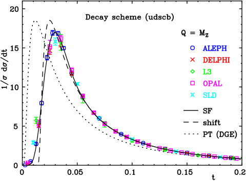
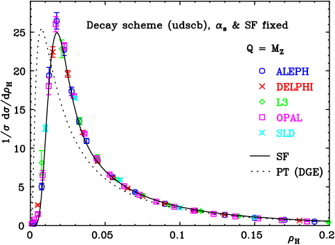
Figure 7: Event-shape distributions: theory vs. data. The thrust (left) and the heavy–jet–mass (right) distributions, computed by DGE Gardi:2002bg for center-of-mass energy of $Q=M_{Z}$, are compared with LEP and SLD data. In the thrust case the three lines show: a Principal Value DGE calculation with no power corrections (dots); one which is shifted, where the shift parameter is determined is a global fit to data (dashed); and one that includes higher power corrections, determined in a fit (full line). These corrections are found to be consistent with the predication that the width does not change due to hadronization. In the heavy–jet–mass case no additional fits are performed: the dotted line is the result of a Principal Value DGE calculation and the full line includes hadronization corrections based on the fit to the thrust.

As shown in Table 1 the single–dressed–gluon calculation predicts the absence of renormalons at all integer values of $u$; it therefore predicts only odd power corrections ${\cal O}\left((N\Lambda/Q)^{k}\right)$ in the exponent. The ensuing phenomenology is the following:

• The leading correction ${\cal O}\left(N\Lambda/Q\right)$, generates a global shift of the distribution and a $\Lambda/Q$ correction to average values of event–shape variables. This idea Webber:1994cp –BM quickly and led to successful phenomenology: the shift can be described in terms of a single, approximately universal non-perturbative parameter in a large class of distributions Dasgupta:2003iq .

• When approaching the threshold region, conventional Sudakov resummation accompanied by a shift of the distribution was proven insufficient. Here DGE DGE_thrust ; Gardi:2002bg made the difference. As shown in Fig. 7 the shape of the (Principal Value) DGE calculation, before any power corrections are included, is already very close to that of the data. Specifically, the width of the distribution is very similar, in accordance with the renormalon prediction that an ${\cal O}\left((N\Lambda/Q)^{2}\right)$ correction would not occur.

A dedicated DGE–based analysis in Ref. Gardi:2002bg has demonstrated that the measured hadronization effects are consistent with the renormalon predictions for power corrections. Successful fits to experimental data have been performed over the entire two–jet region and over a large range of energies. Moreover, as shown in Fig. 7, the relation between hadronization corrections to different shape variables has been tested well into the threshold region.

It is worthwhile noting that the value of $\alpha_{s}^{\hbox{\tiny${\overline{\rm MS}}$}}(M_{Z})$ extracted from fits to the thrust distribution employing DGE Gardi:2002bg (or from the average thrust, employing renormalon resummation Gardi:1999dq ) is consistently lower than the world average value (by about $7\%$). The theoretical uncertainty (estimated Gardi:2002bg as $\pm 5\%$) is significantly larger than the experimental one ($\pm 1\%$), and it is dominated by uncertainty due to higher–order perturbative corrections. It is therefore important to revisit the comparison with data once ${\cal O}(\alpha_{s}^{3})$ calculations Gehrmann-DeRidder:2006hm become available.

An important comment is that in contrast with other distributions considered here, event–shape distributions are not completely inclusive Nason:1995hd ; Milan . For example, the thrust and the heavy–jet–mass distributions are defined based on the separation of space into two hemispheres. The single–dressed–gluon calculation of the Sudakov exponent, on which the power–correction analysis is based, assumes that the momentum of final–state particles associated with a single off-shell gluon is restricted to one hemisphere. This means in particular that certain correlations between the masses of the two hemispheres are neglected. The no-correlation assumption is also used when relating Gardi:2002bg the thrust and the heavy–jet–mass distributions as shown in Fig. 7 above. The successful comparison with data indicates that these correlations are indeed small in the two–jet limit.

IV.3 Heavy–quark fragmentation

Consider next the fragmentation process in which an off-shell heavy quark of mass $m$, produced at high energy ${\cal O}(Q)$, fragments into a heavy hadron. This process is infrared and collinear safe. Therefore, the fragmentation function can be computed in perturbation theory, assuming that the final state is an on-shell heavy quark Nason:1996pk ; CC ; CG ; Gardi:2003ar . This perturbative fragmentation function differs from the physical one by power corrections  Nason:1996pk ; CC .

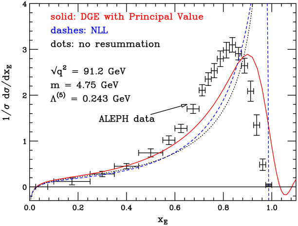
Figure 8: Heavy–quark fragmentation: perturbation theory vs. data. Comparison between perturbative calculations CG of the normalized differential distribution in $e^{+}e^{-}\longrightarrow b+X$ with respect to $x_{E}\equiv 2E/Q$, and experimental data from Aleph. The dotted line is based on a simple NLO calculation with no soft–gluon resummation: only evolution logarithms $\ln(m^{2}/Q^{2})$ are resummed; the dashed line includes in addition soft–gluon resummation to NLL accuracy; the full line is the corresponding DGE result computed with the Principal Value prescription (the DGE Sudakov factor is quoted in Eq. (27) above).

Traditionally, heavy–quark fragmentation effects have been described in terms of “fragmentation functions” Peterson ; Kart , a given functional form with one or more free parameters. Upon excluding the difficult threshold region where the fragmentation function peaks, such fits can indeed be performed. However, since there is no direct relation between these models and the QCD definition of the fragmentation function, the universality of the extracted parameters is doubtful. Within the threshold region such fragmentation models simply fail to bridge the gap between the resummed perturbative calculation and the data. This provided a strong incentive to apply the DGE approach to this problem CG ; Gardi:2003ar .

As shown in Table 1, power–correction analysis of the Sudakov exponent in the large–$\beta_{0}$ limit has definite predictions:

• The leading infrared renormalon is located at $u=\frac{1}{2}$. Therefore, one expects a global shift of the distribution in $x_{E}$ going from the partonic to the hadronic level. Comparing the data to the Principal value DGE result in Fig. 8, one indeed observes such a shift. The shift parameter $\epsilon_{1}^{\rm PV}$ in Eq. (IV) can of course be determined by fitting the data, as shown in Fig. 9 below.

• The $u=1$ renormalon is absent. Therefore, one expects that the width of the spectrum would not be modified by non-perturbative fragmentation effects. Again, this is confirmed by the data CG ; see Figs. 8 and 9 below.

• Higher renormalon ambiguities at $u=\frac{3}{2}$ and above are present, and therefore higher–power corrections are expected. Their effect is restricted to high moments CG .

Fits performed in Ref. CG confirm that Eq. (IV) above with a couple of leading non-perturbative power corrections, yields an excellent description of experimental data to very high moments. As shown in Fig. 9, a good description of data (and a consistent determination of $\alpha_{s}$) is achieved already with a single non-perturbative parameter, a plain shift of the PV-regularized DGE result. It should be emphasized that such power–correction phenomenology could not be developed starting with fixed–order calculations or fixed–logarithmic–accuracy Sudakov resummation: as shown in Fig. 8 there is a qualitative difference between these results and the DGE one.

Figure 9: Heavy–quark fragmentation: DGE–based fit to heavy–meson production data from LEP. Left: results of a fit for $\Lambda$ (i.e. $\alpha_{s}$) and $\epsilon_{1}^{\rm PV}$ in Eq. (IV) (setting $\epsilon_{k}^{\rm PV}=0$ for $k\geq 2$) to Aleph moments $N=2$ to $6$. Right: the corresponding curve in $x_{E}$ space, compared to the Aleph and Delphi data.

IV.4 Inclusive decay spectra

As discussed in Sec. II, the application of DGE to inclusive B decay spectra has been very successful. The most striking fact is that the on-shell approximation directly provides a good approximation of the spectrum. In other words, at present accuracy, power corrections on the soft scale ${\cal O}\left((N\Lambda/Q)^{k}\right)$, the ones that distinguish between the quark distribution in a meson and that in an on-shell quark BDK , are negligible.

To understand this issue, let us return once more to Table 1:

• As in the case of heavy–quark fragmentation (as well as in event-shape distributions) the leading infrared renormalon in the Sudakov exponent is located at $u=\frac{1}{2}$. However, a unique property of inclusive decay spectra, is that this ambiguity cancels out exactly upon computing the resummed spectrum in physical kinematic variables BDK ; Andersen:2005bj ; Andersen:2005mj ; QD ; Gardi:2005mf . For example, for the radiative decay the resummed on-shell calculation yields:

  $$\left.\frac{1}{\Gamma_{\rm tot}}\frac{d\Gamma}{dE_{\gamma}}\right|_{\rm res} = \frac{2}{m_{b}}\int_{c-i\infty}^{c+i\infty}\frac{dN}{2\pi i}\left(\frac{2E_{\gamma}}{m_{b}}\right)^{-N}\left[H(m_{b})\underbrace{J_{N}(m_{b};\mu_{F})\,\times\,S_{N}(m_{b};\mu_{F})}_{{\rm Sud}(m_{b},N)}\,+\,\,{\cal O}(1/N)\right]$$ (30)

  Here $S_{N}(m_{b};\mu_{F})$ is the solution of Eq. (25), the Sudakov factor describing the momentum distribution in an on-shell b quark. It has a leading ambiguity of the form $\exp\left\{\pm(N-1)\Lambda/m_{b}\right\}$. The mass appearing in the inverse Mellin transformation in (30) is the pole mass, which also has a leading renormalon ambiguity Bigi:1994em ; Beneke:1994sw at $u=\frac{1}{2}$. Since the mass is raised to the power $N-1$, it generates an ambiguity of the form $\exp\left\{\mp(N-1)\Lambda/m_{b}\right\}$ in Eq. (30), which cancels against the ambiguity of $S_{N}(m_{b};\mu_{F})$. This cancellation was confirmed by explicit calculations of the corresponding renormalon residues in the large–$\beta_{0}$ limit (Sec. 2.2.3 in Ref. BDK ).
  Eq. (30) refers specifically to the radiative decay, in which case the meson mass does not enter the calculation. A similar cancellation occurs in other inclusive distribution, see e.g. Eq. (4.4) in Ref. Andersen:2005mj for the charmless semileptonic decay. There the ambiguity cancels upon expressing the partonic kinematic variables in terms of hadronic ones, a transformation that involves the mass difference between the meson and the quark.

• As in the heavy–quark–fragmentation and event–shape–distribution examples considered above, the $u=1$ renormalon in Eq. (25) is absent. Therefore, one expects that the width of the spectrum would not be modified by non-perturbative Fermi–motion effects. Also here, comparison with data confirms the renormalon prediction: the photon–energy variance in Fig. 3, computed as a function of the cut, is well described by the on-shell approximation.

• Finally, there are renormalon ambiguities at $u=\frac{3}{2}$ and above, which imply that non-perturbative power corrections due to Fermi motion should be included in Eq. (IV) with $k\geq 3$. These should have an effect for high moments $N\sim m_{b}/\Lambda$. Given the factorial suppression of high powers in Eq. (IV), a few non-perturbative parameters would be sufficient for any practical purpose, even if very precise data become available.

The obvious conclusion is that having sufficient control on the perturbative calculation and the parametric form of power corrections, the parametrization of the “shape function” and the associated uncertainty can be completely avoided.

V Conclusions

The QCD calculation of inclusive cross sections and decay spectra near kinematic thresholds is challenging because of large perturbative and non-perturbative corrections. Conventional Sudakov resummation is limited to the range where non-perturbative corrections are negligible. The DGE approach has proven effective in extending the range of applicability of perturbation theory well into the threshold region, where non-perturbative corrections are relevant. DGE makes maximal use of the known all–order structure of the Sudakov exponent and the inherent infrared safety of the observable. The main characteristics of this formalism are:

• Factorization and exponentiation in moment space, going beyond the perturbative (logarithmic) level.

• Resummation of running–coupling effects using Borel summation, leading to renormalization–group invariance of the Sudakov exponent.

• Power–like separation between the perturbative result of the exponent, computed as the Principal Value Borel sum and non-perturbative power corrections, whose parametric form is deduced from the renormalon residues.

DGE has a high predictive power:

• Important features of the distribution are captured by resummed perturbation theory.

• The perturbative result is modified by non-perturbative power corrections of a definite parametric form, see Eqs. (• ‣ III) and (IV). The power–correction expansion in (IV) converges well even for high moments, and thus a small number of non-perturbative parameters is sufficient.

The main underlying assumption, whose validity cannot be addressed within perturbation theory, is that the dominant non-perturbative effects in the threshold region are indeed the ones identified by renormalon ambiguities. Here comparison with experimental data is essential. In all inclusive distributions considered so far, the observed pattern of power corrections is consistent with the renormalon prediction. Specifically,

• The potentially leading, $u=\frac{1}{2}$ renormalon ambiguity in the “soft” Sudakov exponent $S_{N}(Q;\mu_{F})$ is of ${\cal O}\big{(}(N-1)\Lambda/Q\big{)}$. This corresponds to a global shift of the resummed distribution upon going from the partonic to the hadronic level. This shift has been firmly established and measured in event–shape distributions DGE_thrust ; Gardi:2002bg (see also Dasgupta:2003iq ; Dokshitzer:1997ew ; Korchemsky:1995zm ) and in heavy–quark fragmentation CG . In Drell–Yan or Higgs production the $u=\frac{1}{2}$ renormalon is absent due to a specific symmetry property of the corresponding anomalous dimension, which can be deduced Beneke:1995pq ; Gardi:2001di from Eq. (26) and Table. 1 above (see an alternative approach in Ref. Laenen:2000ij ). In inclusive decay spectra the $u=\frac{1}{2}$ ambiguity cancels out within the on-shell approximation, upon expressing the spectrum in terms of hadronic momenta BDK ; Andersen:2005bj ; Andersen:2005mj .

• The potential $u=1$ renormalon ambiguity does not occur in several cases, owing to symmetry properties of the Sudakov anomalous dimensions, which can be deduced from Eq. (26) and Table. 1. The corresponding non-perturbative correction would have induced an ${\cal O}(1)$ change in the width of the spectra. Such effects have been excluded by comparison with data in event–shape distributions (see Ref. DGE_thrust ; Gardi:2002bg and Fig. 7 above), heavy–quark fragmentation (see Ref. CG and Fig. 8 and 9 above) and inclusive decay spectra (see Ref. Gardi:2005mf and the variance plot in Fig. 3 above).

The recent application of DGE to inclusive decay spectra has led to a fundamental change in the perception of the predictive power of resummed perturbation theory. For over a decade, it has been repeatedly stated that the calculation of the $\bar{B}\longrightarrow X_{s}\gamma$ and $\bar{B}\longrightarrow X_{u}l\bar{\nu}$ spectra is strictly beyond the limits of perturbation theory. The description of the spectra in the peak region has been based on “shape–function” phenomenology, where an arbitrary functional form is introduced whose first few moments are constrained by data. Refs. BDK ; Gardi:2004gj ; Andersen:2005bj ; Andersen:2005mj ; QD ; Gardi:2005mf have shown that resummed perturbation theory provides a good approximation to these spectra while genuinely non-perturbative effects (Eq. (IV) with $k\geq 3$) due to the “primordial” Fermi motion are not large. This advancement is already reflected in precision determination of $m_{b}^{\hbox{\tiny${\overline{\rm MS}}$}}$ and $|V_{\rm ub}|$ using measurements of the B factories HFAG . Moreover, in this framework there are high prospects for improving the determination of these parameters by incorporating higher–order (NNLO) calculations and by quantifying the relevant non-perturbative corrections.