Geometric scaling in diffractive deep inelastic scattering

Abstract

The geometric scaling property observed in the HERA data at small $x,$ that the deep inelastic scattering (DIS) total cross-section is a function of only the variable $Q^{2}x^{\lambda},$ has been argued to be a manifestation of the saturation regime of QCD and of the saturation scale $Q^{2}_{s}(x)\!\sim\!x^{-\lambda}.$ We show that this implies a similar scaling in the context of diffractive DIS and we observe, for several diffractive observables, that the experimental data from HERA confirm the expectations of this scaling.

I Introduction

Deep inelastic scattering (DIS) is a process in which a virtual photon is used as a hard probe to resolve the small distances inside a proton and study its partonic constituents: quarks and gluons that obey the laws of perturbative QCD. When probing with a fixed photon virtuality $Q^{2}\!\gg\!\Lambda_{QCD}^{2},$ and increasing the energy of the photon-proton collision $W$, the parton densities inside the proton grow. Eventually, at some energy much bigger than the hard scale, corresponding to a small value of $x\!=\!Q^{2}/W^{2}$, one enters the saturation regime of QCD glr : the gluon density becomes so large that non-linear effects like gluon recombination become important, taming the growth of the parton densities.

The transition to the saturation regime is characterized by the so-called saturation momentum $Q_{s}(x)\!=\!Q_{0}\ x^{-\lambda/2}.$ This is an intrinsic scale of the high-energy proton which increases as $x$ decreases. $Q_{0}\!\sim\!\Lambda_{QCD},$ but as the energy increases, $Q_{s}$ becomes a hard scale, and the transition to saturation occurs when $Q_{s}$ becomes comparable to $Q.$ The higher $Q^{2}$ is, the smaller $x$ should be to enter the saturation regime.

Although the saturation regime is only reached when $Q_{s}\!\sim\!Q,$ observables are sensitive to the saturation scale already during the approach to saturation extscal when $\Lambda_{QCD}\!\ll\!Q_{s}\!\ll\!Q.$ For inclusive events in deep inelastic scattering, this feature manifests itself via the so-called geometric scaling property: instead of being a function of $Q^{2}/Q_{0}^{2}$ and $x$ separately, the total cross-section is only a function of $\tau\!=\!Q^{2}/Q_{s}^{2}(x),$ up to large values of $\tau.$ Experimental measurements of inclusive DIS are compatible with that prediction geoscal .

Part of the DIS events are diffractive, meaning that the proton remains intact after the collision and that there is a rapidity gap between that proton and the rest of the final-state particles. Such events are expected to be much more sensitive to the saturation regime of QCD than the inclusive ones golec and our goal in this letter is to extend the geometric scaling property to diffractive DIS and to compare the resulting predictions with the available experimental data. We shall consider several diffractive observables, focusing on inclusive hard diffraction and vector-meson production.

In the saturation regime of QCD, contributions to the cross-sections growing like $Q_{s}/Q$ are important. The leading-twist approximation of perturbative QCD, in which $Q^{2}$ is taken as the bigger scale, cannot account for such contributions, and therefore is not appropriate to describe the small-x limit of deep inelastic scattering. As leading-twist gluon distributions cannot be used to compute cross-sections, the dipole picture of DIS dipole has been developed to describe the high-energy limit. It expresses the hadronic scattering of the virtual photon through its fluctuation into a color singlet $q\bar{q}$ pair (or dipole) of a transverse size $r\!\sim\!1/Q$. The dipole is then the hard probe that resolves the small distances inside the proton.

The dipole picture naturally incorporates the description of both inclusive and diffractive events into a common theoretical framework nikzak ; biapesroy , as the same dipole scattering amplitudes enter in the formulation of the inclusive and diffractive cross-sections. This will be recalled in Section II and will allow us to extend the geometric scaling property to diffractive observables, as detailed in Section III. Finally, Section IV is devoted to comparison with experimental data and Section V concludes.

II The dipole picture of deep inelastic scattering

We focus on diffractive DIS: $\gamma^{*}p\!\rightarrow\!Xp.$ The proton gets out of the $\gamma^{*}\!-\!p$ collision intact, and there is a rapidity gap between that proton and the final state $X$ whose invariant mass we denote $M_{X}.$ We recall that the photon virtuality is denoted $Q^{2},$ and the $\gamma^{*}\!-\!p$ total energy $W.$ It is convenient to introduce the following variables:

$$x=\frac{Q^{2}}{Q^{2}+W^{2}}\ ,\hskip 28.45274pt\beta=\frac{Q^{2}}{Q^{2}+M_{X}^{2}}\ ,\hskip 28.45274ptx_{\mathbb{P}}=x/\beta\ .$$ (1)

The $\gamma^{*}\!-\!p$ total cross-section $\sigma^{\gamma^{*}p\rightarrow X}_{tot}$ is usually expressed as a function of $x$ and $Q^{2},$ while the diffractive cross-section $d\sigma^{\gamma^{*}p\rightarrow Xp}_{diff}/d\beta$ is expressed as a function of $\beta,$ $x_{\mathbb{P}},$ and $Q^{2}.$ Note that the size of the rapidity gap in the final state is $\ln(1/x_{\mathbb{P}}).$

To compute those cross-sections in the high-energy limit, it is convenient to view the process in a particular frame called the dipole frame. In this frame, the virtual photon undergoes the hadronic interaction via a fluctuation into a colorless $q\bar{q}$ pair, called dipole, which then interacts with the target proton. The wavefunctions $\psi_{\lambda}^{f,\alpha\beta}(z,\textbf{r};Q^{2})$ describing the splitting of a virtual photon with polarization $\lambda$ into a dipole are well known. The indices $\alpha$ and $\beta$ denote the spins of the quark and the antiquark composing the dipole of flavor $f.$ The wavefunctions depend on $Q^{2},$ the fraction $z$ of longitudinal momentum (with respect to the $\gamma^{*}\!-\!p$ collision axis) carried by the quark, and the two-dimensional vector r whose modulus is the transverse size of the dipole (transverse coordinates are obtained from a Fourier transform of transverse momenta). Formulae giving the funcions $\psi_{\lambda}^{f,\alpha\beta}$ can be found in the literature (see for instance biapesroy ). In what follows, we will need the functions $\Phi^{f}_{\lambda}$ which describe the overlap between two wavefunctions for splitting into dipoles of different transverse size r and $\textbf{r}^{\prime}:$

$$\phi^{f}_{\lambda}(z,\textbf{r},\textbf{r}^{\prime};Q^{2})=N_{c}\sum_{\alpha\beta}\left[\psi_{\lambda}^{f,\alpha\beta}(z,\textbf{r}^{\prime};Q^{2})\right]^{*}\psi_{\lambda}^{f,\alpha\beta}(z,\textbf{r};Q^{2})\ .$$ (2)

For a transversely (T) or longitudinally (L) polarized photon, these functions are given by

$$\phi^{f}_{T}(z,\textbf{r},\textbf{r}^{\prime};Q^{2})=\frac{\alpha_{em}N_{c}}{2\pi^{2}}e_{f}^{2}\left((z^{2}+(1-z)^{2})\varepsilon_{f}^{2}\frac{\textbf{r}.\textbf{r}^{\prime}}{|\textbf{r}||\textbf{r}^{\prime}|}K_{1}(\varepsilon_{f}|\textbf{r}|)K_{1}(\varepsilon_{f}|\textbf{r}|^{\prime})+m_{f}^{2}K_{0}(\varepsilon_{f}|\textbf{r}|)K_{0}(\varepsilon_{f}|\textbf{r}|^{\prime})\right)\ ,$$ (3)

$$\phi^{f}_{L}(z,\textbf{r},\textbf{r}^{\prime};Q^{2})=\frac{\alpha_{em}N_{c}}{2\pi^{2}}e_{f}^{2}4Q^{2}z^{2}(1-z)^{2}K_{0}(\varepsilon_{f}|\textbf{r}|)K_{0}(\varepsilon_{f}|\textbf{r}|^{\prime})\ .$$ (4)

In the above, $e_{f}$ and $m_{f}$ denote the charge and mass of the quark with flavor $f$ and $\varepsilon_{f}^{2}\!=\!z(1\!-\!z)Q^{2}\!+\!m_{f}^{2}.$

The total cross-section $\sigma^{\gamma^{*}p\rightarrow X}_{tot}.$ Via the optical theorem, it is related to the elastic scattering of the virtual photon. In the dipole frame, this scattering happens as follows: at a given impact parameter $\textbf{b},$ the photon splits into a dipole with a given size r which scatters elastically off the proton and recombines back into the photon. Therefore the overlap function $\Phi_{\lambda}^{\gamma^{*}\gamma^{*}}$ which enters in the computation of the total cross-section is

$$\Phi_{\lambda}^{\gamma^{*}\gamma^{*}}(z,|\textbf{r}|;Q^{2})=\sum_{f}\phi^{f}_{\lambda}(z,\textbf{r},\textbf{r};Q^{2})\ .$$ (5)

The total cross-section is then given by (for fixed impact parameter b):

$$\frac{d\sigma^{\gamma^{*}p\rightarrow X}_{tot}}{d^{2}b}(x,Q^{2})=2\int d^{2}r\int_{0}^{1}dz\sum_{\lambda=L,T}\Phi_{\lambda}^{\gamma^{*}\gamma^{*}}(z,|\textbf{r}|;Q^{2})\ T_{q\bar{q}}(\textbf{r},\textbf{b};x)$$ (6)

where the function $T_{q\bar{q}}(\textbf{r},\textbf{b};x)$ is the elastic scattering amplitude of the dipole of size r off the proton at impact parameter $\textbf{b}.$ It contains the $x$ dependence, reflecting the fact that in our frame, the proton carries all the energy and is therefore evolved up to the rapidity $\ln(1/x).$ In the high-energy limit $x\!\ll\!1$ we are considering here, $T_{q\bar{q}}$ does not depend on $z.$

The diffractive cross-section $d\sigma^{\gamma^{*}p\rightarrow Xp}_{diff}/d\beta.$ In the amplitude, the photon splits into a dipole of size r which scatters off the proton and dissociates into a final state of invariant mass $M_{X}.$ The same happens in the complex conjugate amplitude, except that the dipole size $\textbf{r}^{\prime}$ is different from $\textbf{r}.$ Indeed, the final state is characterized by a particular value of $M_{X}$ (or equivalently $\beta$), corresponding to a particular momentum of the quark-antiquark pair. In coordinate space, this imposes two different dipole sizes in the amplitude and the complex conjugate amplitude, therefore the functions $\phi_{\lambda}^{f}(z,\textbf{r},\textbf{r}^{\prime};Q^{2})$ (see (2)) enter in the computation of the diffractive cross-section:

$$\frac{d\sigma^{\gamma^{*}p\rightarrow Xp}_{diff}}{d^{2}b\ d\beta}(\beta,x_{\mathbb{P}},Q^{2})=\frac{Q^{2}}{4\pi\beta^{2}}\sum_{f}\int d^{2}r\int d^{2}r^{\prime}\int_{0}^{1}dzz(1-z)\Theta(\boldsymbol{\kappa}_{f}^{2})\ e^{i\boldsymbol{\kappa}_{f}.(\textbf{r}^{\prime}-\textbf{r})}\hskip 85.35826pt$$

$$\sum_{\lambda=L,T}\phi_{\lambda}^{f}(z,\textbf{r},\textbf{r}^{\prime};Q^{2})T_{q\bar{q}}(\textbf{r},\textbf{b};x_{\mathbb{P}})T_{q\bar{q}}(\textbf{r}^{\prime},\textbf{b};x_{\mathbb{P}})\ .$$ (7)

In the above, $\boldsymbol{\kappa}_{f}^{2}\!=\!z(1\!-\!z)Q^{2}(1\!-\!\beta)/\beta\!-\!m_{f}^{2}.$ Note that now, the proton is only evolved up to the rapidity $\ln(1/x_{\mathbb{P}}).$ This is because some of the energy ($M_{X}^{2}$) is carried by the dipole in order to form the diffractive final state. The dipole is evolved up to a rapidity $\ln(1/\beta)$ and the proton up to the rapidity $\ln(\beta/x)\!=\!\ln(1/x_{\mathbb{P}}).$ The high-energy limit in this case is $x_{\mathbb{P}}\!\ll\!1.$

To write formula (7), we have neglected possible final states containing gluons. This is justified because these are suppressed by extra powers of $\alpha_{s}.$ However, if $\beta$ becomes too small, the dipole evolves to higher rapidities and emits soft gluons. Large logarithms $\alpha_{s}\ln(1/\beta)$ coming from the emission of those soft gluons arise, and multiple gluons emissions should be resummed to complete formula (7). These multiple gluon emissions in the limit $\beta\ll 1$ can also be accounted for in the dipole picture diffscal , provided one uses the large$-N_{c}$ limit. Indeed in this limit, a dipole emitting a soft gluon is equivalent to a dipole splitting into two dipoles. To illustrate this, the contribution of the $q\bar{q}g$ final state reads (see also gbar ; gkop ; gkov ; gmun ; gmar ):

$$\frac{d\sigma^{\gamma^{*}p\rightarrow(X\!=\!q\bar{q}g)p}_{diff}}{d^{2}b\ d\beta}=\frac{\alpha_{s}N_{c}}{2\pi^{2}\beta}\int d^{2}r\int_{0}^{1}dz\sum_{\lambda=L,T}\Phi_{\lambda}^{\gamma^{*}\gamma^{*}}(z,|\textbf{r}|;Q^{2})\int d^{2}z\frac{\textbf{r}^{2}}{\textbf{z}^{2}(\textbf{r}\!-\!\textbf{z})^{2}}\Big{[}T^{(2)}_{q\bar{q}}(\textbf{z},\textbf{r}\!-\!\textbf{z},\textbf{b};x_{\mathbb{P}})-T_{q\bar{q}}(\textbf{r},\textbf{b};x_{\mathbb{P}})\Big{]}^{2}\ .$$ (8)

In the above, the function $T^{(2)}_{q\bar{q}}(\textbf{z},\textbf{r}\!-\!\textbf{z},\textbf{b};x_{\mathbb{P}})$ is the scattering amplitude for two dipoles of sizes z and $\textbf{r}\!-\!\textbf{z}$ at impact parameters $\textbf{b}\!-\!(\textbf{r}\!-\!\textbf{z})/2$ and $\textbf{b}\!-\!\textbf{z}/2$ respectively. These come from the splitting of the dipole of size r at impact parameter $\textbf{b}.$ Moreover the overlap function is $\Phi_{\lambda}^{\gamma^{*}\gamma^{*}}.$ It is so because in the leading $\ln(1/\beta)$ approximation, the final state mass $M_{X}$ is fixed only by the soft gluon longitudinal momentum, and therefore transverse sizes are the same in the amplitude and the complex conjugate amplitude.

The diffractive vector-meson production cross-section $\sigma^{\gamma^{*}p\rightarrow Vp}_{VM}.$ In this case, after scattering off the proton, the dipole recombines into a particular final state $X\!=\!V$, a vector meson whose mass we shall denote $M_{V}.$ To describe this process, we need to introduce the wavefunction $\varphi_{\lambda}^{f,\alpha\beta}(z,\textbf{r};M_{V}^{2})$ which describes the splitting of the vector meson with polarization $\lambda$ into the dipole. The overlap function $\Phi^{\gamma^{*}V}_{\lambda}$ which enters in the computation of the vector-meson production amplitude is then given by

$$\Phi^{\gamma^{*}V}_{\lambda}(z,|\textbf{r}|;Q^{2},M_{V}^{2})=\sum_{f\alpha\beta}\left[\varphi_{\lambda}^{f,\alpha\beta}(z,\textbf{r};M_{V}^{2})\right]^{*}\psi_{\lambda}^{f,\alpha\beta}(z,\textbf{r};Q^{2})\ .$$ (9)

Because the final state has been explicitely projected into a vector meson, the two dipoles in the amplitude and the complex conjugate amplitude are not connected and the cross-section (for fixed impact parameter) is simply the square of the amplitude:

$$\frac{d\sigma^{\gamma^{*}p\rightarrow Vp}_{VM}}{d^{2}b}(x_{\mathbb{P}},Q^{2})=\left|\int d^{2}r\int_{0}^{1}dz\sum_{\lambda=L,T}\Phi_{\lambda}^{\gamma^{*}V}(z,|\textbf{r}|;Q^{2},M_{V}^{2})\ T_{q\bar{q}}(\textbf{r},\textbf{b};x_{\mathbb{P}})\right|^{2}\ .$$ (10)

The functions $\Phi^{\gamma^{*}V}_{\lambda}$ depend on the meson wavefunctions $\varphi_{\lambda}^{f,\alpha\beta},$ and several different models exist in the literature mwfs1 ; mwfs2 ; mwfs3 . As emphasized later, we shall only use model-independent features of $\Phi^{\gamma^{*}V}_{\lambda}.$ Formula (10) can be used to compute the Deeply-Virtual-Compton-Scatering (DVCS) cross-section $\sigma^{\gamma^{*}p\rightarrow\gamma p}_{DVCS},$ provided one uses the overlap function

$$\Phi^{\gamma^{*}\gamma}_{T}(z,|\textbf{r}|;Q^{2})=\sum_{f\alpha\beta}\left[\psi_{T}^{f,\alpha\beta}(z,\textbf{r};0)\right]^{*}\psi_{T}^{f,\alpha\beta}(z,\textbf{r};Q^{2})$$ (11)

between the incoming virtual photon and the outgoing transversely-polarized real photon.

III Saturation, geometric scaling and its consequences

Using the dipole picture of deep inelastic scattering, we have expressed the total (6), diffractive (7) and exclusive vector-meson production (10) cross-sections in the high-energy limit in terms of a single object: the dipole scattering amplitude off the proton $T_{q\bar{q}}(\textbf{r},\textbf{b};x).$ It is mainly a non-perturbative quantity, but its evolution towards small values of $x$ (or high energy) is computable from perturbative QCD. Evolution equations have been established in the leading $\ln(1/x)$ approximation bk ; jimwlk and, at least for central impact parameter, one has learned a lot about the growth of the dipole amplitude and the transition from the leading-twist regime $T_{q\bar{q}}\!\ll\!1$ towards and into the saturation regime $T_{q\bar{q}}\!=\!1.$

The most important prediction was probably the geometric scaling regime extscal ; tw : at small values of $x,$ instead of being a function of a priori the two variables r and $x,$ $T_{q\bar{q}}(\textbf{r},\textbf{b}\!\simeq\!0;x)$ is actually a function of the single variable $\textbf{r}^{2}Q^{2}_{s}(x)$ up to inverse dipole sizes significantly larger than the saturation scale $Q_{s}(x).$ In formulae, one can write

$$T_{q\bar{q}}(\textbf{r},\textbf{b};x)=S(\textbf{b})\ T(\textbf{r}^{2}Q^{2}_{s}(x))$$ (12)

where we have introduced the impact parameter profile $S(\textbf{b}).$ Typically, $S(\textbf{b})\!=\!e^{-\textbf{b}^{2}/R_{p}^{2}}$ where $R_{p}$ is the transverse radius of the proton. When performing the b integration in formulae (6), (7) or (10), this contributes only to the normalization via a constant factor $\int d^{2}b\ S(\textbf{b})\!=\!S_{p},$ caracterising the transverse area of the proton. If $\textbf{r}^{2}Q^{2}_{s}\!>\!1$ then $T\!=\!1$ and the scaling is obvious. We insist that the scaling property (12) is a non-trivial prediction for $\textbf{r}^{2}Q^{2}_{s}\!\ll\!1,$ when $T$ is still much smaller that 1. Of course the geometric scaling window has a limited extension: at very small dipole sizes, deep into the leading-twist regime, the scaling breaks down. Universal scaling violations tw due to $x$ not being small enough have also been derived. Recently, a new type of scaling violations has been predicted ploop ; diffscal , this one eventually arising when $x$ becomes even smaller, transforming the geometric scaling regime into an intermediate energy regime.

In this work, we shall consider the case of exact scaling (12). As already mentioned, the resulting prediction for the DIS total cross-section is in very good agreement with experimental measurements geoscal (see also schild ). Our goal is to further test the geometric scaling regime by considering its prediction for diffractive observables. But, as a reminder, let us start with the total cross-section. Neglecting quark masses, one can rewrite the cross-section (6) as

$$\sigma^{\gamma^{*}p\rightarrow X}_{tot}(x,Q^{2})=2S_{p}\frac{\alpha_{em}N_{c}}{\pi}\sum_{f}e_{f}^{2}\int_{0}^{\infty}\bar{r}d\bar{r}\int_{0}^{1}dz\left\{f_{T}(z)K_{1}^{2}(\sqrt{z(1\!-\!z)}\bar{r})+f_{L}(z)K_{0}^{2}(\sqrt{z(1\!-\!z)}\bar{r})\right\}T{\left({\frac{Q^{2}_{s}(x)}{Q^{2}}\ \bar{r}^{2}}\right)}$$ (13)

where we have introcuced the functions $f_{T}(z)\!=\!(z^{2}+(1\!-\!z)^{2})z(1\!-\!z)$ and $f_{L}(z)\!=\!4z^{2}(1\!-\!z)^{2}$ and rescaled the size variable $|\textbf{r}|$ to the dimensionless variable $\bar{r}\!=\!Q|\textbf{r}|.$ We obtain the geometric scaling of the total cross-section at small $x:$

$$\sigma^{\gamma^{*}p\rightarrow X}_{tot}(x,Q^{2})=\sigma^{\gamma^{*}p\rightarrow X}_{tot}(\tau)\ ,\hskip 28.45274pt\tau=Q^{2}/Q_{s}^{2}(x)\ .$$ (14)

This has been seen confirmed by experimental data geoscal with $Q_{s}(x)$ given by

$$Q_{s}(x)=Q_{0}{\left({\frac{x}{x_{0}}}\right)}^{-\lambda/2}\ ,\hskip 14.22636ptQ_{0}\equiv 1\mbox{GeV}$$ (15)

and the parameters $\lambda\!=\!0.288$ and $x_{0}\!=\!3.04\ 10^{-4}$ taken from golec . In order to illustrate it, Fig.1 is an update of the original plot which shows the cross-section $\sigma^{\gamma^{*}p\rightarrow X}_{tot}$ as a function of $\tau$ with the latest data of the different experiments which provide measurements at $x\!<\!0.01:$ the H1 h1f2 , ZEUS zeusf2 , E665 e665f2 and NMC nmcf2 collaborations. Except for one E665 point, the data do lie on the same curve. This is even true at low values of $Q^{2},$ for which one could have expected scaling violations do to the charm quark mass, but one can see on Fig.1 that these are not sizable (see also gonmac ).

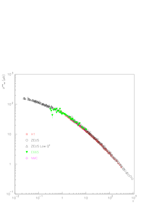
Figure 1: The total cross section $\sigma^{\gamma^{*}p\rightarrow X}_{tot}$ as a function of $\tau$ for $x\!<\!0.01.$ The data are the most recent by the H1, ZEUS, E665 and NMC collaborations. Only statistical uncertainties are shown.

Let us now consider the diffractive cross-section (7). It can be rewritten

$$\frac{d\sigma^{\gamma^{*}p\rightarrow Xp}_{diff}}{d\beta}(\beta,x_{\mathbb{P}},Q^{2})=S_{p}\frac{\alpha_{em}N_{c}}{2\pi\beta^{2}}\sum_{f}e_{f}^{2}\int_{0}^{1}dzz(1-z)\sum_{\lambda=L,T}f_{\lambda}(z)I^{2}_{\lambda}(z,\beta,Q^{2}_{s}(x_{\mathbb{P}})/Q^{2})$$ (16)

with the following integral

$$I_{T,L}(z,\beta,Q^{2}_{s}/Q^{2})=\int_{0}^{\infty}\bar{r}d\bar{r}K_{1,0}(\sqrt{z(1\!-\!z)}\bar{r})J_{1,0}(\sqrt{z(1\!-\!z)(1\!-\!\beta)/\beta}\bar{r})T{\left({\frac{Q^{2}_{s}}{Q^{2}}\ \bar{r}^{2}}\right)}$$ (17)

where $I_{T}$ contains $K_{1}$ and $J_{1}$ bessel functions and $I_{L}$ contains $K_{0}$ and $J_{0}.$ So, another signature of the saturation regime of QCD should then be the geometric scaling of the diffractive cross-section at fixed $\beta$ and small $x_{\mathbb{P}}:$

$$\frac{d\sigma^{\gamma^{*}p\rightarrow Xp}_{diff}}{d\beta}(\beta,x_{\mathbb{P}},Q^{2})=\frac{d\sigma^{\gamma^{*}p\rightarrow Xp}_{diff}}{d\beta}(\beta,\tau_{d})\ ,\hskip 28.45274pt\tau_{d}=Q^{2}/Q_{s}^{2}(x_{\mathbb{P}})\ .$$ (18)

This will be discussed in the next Section. Note that for small values of $\beta,$ when using a more complete formulation of the diffractive cross-section, the prediction (18) remains unchanged. For instance, in the geometric scaling regime, the behavior of $T^{(2)}_{q\bar{q}}$ is

$$T^{(2)}_{q\bar{q}}(\textbf{z},\textbf{r}\!-\!\textbf{z},\textbf{b};x)=S(\textbf{b})\tilde{T}(\textbf{z}^{2}Q^{2}_{s}(x),(\textbf{r}\!-\!\textbf{z})^{2}Q^{2}_{s}(x))$$ (19)

and therefore when using formula (8), the prediction (18) remains true and it also the case in other approaches diffscal ; gwus .

Let us finally discuss vector-meson production. In this case, the problem is not as simple because of the extra scale $M_{V}$ and of the model-dependent meson wavefunctions. However, it is possible to take advantage of a quite general feature rather independent of the particular model for the meson wavefunction: longitudinally-polarized vector mesons are predominant and the overlap function follows the approximate scaling law (see for instance mms )

$$2\pi r^{2}\ \int_{0}^{1}dz\ \Phi_{L}^{\gamma V}(z,\textbf{r};Q^{2},M_{V}^{2})\simeq g{\left({\textbf{r}^{2}(Q^{2}+M_{V}^{2})}\right)}$$ (20)

where the function $g$ is sharply picked around 1. As a consequence of this, in the geometric scaling regime the vector-meson production cross-section can be rewritten

$$\sigma^{\gamma^{*}p\rightarrow Vp}_{VM}(x_{\mathbb{P}},Q^{2})=S_{p}\left|\int_{0}^{\infty}\frac{d\bar{r}}{\bar{r}}g(\bar{r}^{2})T{\left({\frac{Q^{2}_{s}(x_{\mathbb{P}})}{Q^{2}+M_{V}^{2}}\bar{r}^{2}}\right)}\right|^{2}$$ (21)

and the following behavior can be predicted:

$$\sigma^{\gamma^{*}p\rightarrow Vp}_{VM}(x_{\mathbb{P}},Q^{2})=\sigma^{\gamma^{*}p\rightarrow Vp}_{VM}(\tau_{V})\ ,\hskip 28.45274pt\tau_{V}=(Q^{2}+M_{V}^{2})/Q_{s}^{2}(x_{\mathbb{P}})\ .$$ (22)

Note that, for the DVCS cross-section, the prediction is $\sigma^{\gamma^{*}p\rightarrow\gamma p}_{DVCS}(x,Q^{2})\!=\!\sigma^{\gamma^{*}p\rightarrow\gamma p}_{DVCS}(\tau)$ without relying on (20).

IV Geometric scaling and diffractive observables

We shall now test the predictions (18) et (22). The H1 and ZEUS experiments at HERA have measured the diffractive cross section for the process $ep\!\rightarrow\!eXY$, selecting events with a large rapidity gap between the systems $X$ and $Y$ in case of H1 f2d97 , and using the so-called $M_{X}$-method in case of ZEUS zeus . $Y$ represents the scattered proton, either intact of in a low-mass excited state, with $M_{Y}\!<\!1.6\ \mbox{GeV}$ (H1) or $M_{Y}\!<\!2.3\ \mbox{GeV}$ (ZEUS). The cut on $t,$ the squared momentum transfer at the proton vertex, is $|t|\!<\!1\ \mbox{GeV}^{2}$ for both experiments. These data are presented in terms of the $t$-integrated reduced cross section $\sigma_{r}^{D(3)}(x_{\rm l\!P},x,Q^{2})$ or the diffractive structure function $F_{2}^{D(3)}(x_{\rm l\!P},x,Q^{2})$ obtained from the relations

$$\frac{d^{3}\sigma^{ep\rightarrow eXY}}{dx_{\rm l\!P}\ dx\ dQ^{2}}=\frac{4\pi\alpha_{em}^{2}}{xQ^{4}}{\left({1-y+\frac{y^{2}}{2}}\right)}\sigma_{r}^{D(3)}(x_{\rm l\!P},x,Q^{2})\hskip 28.45274pt\sigma_{r}^{D(3)}=F_{2}^{D(3)}-\frac{y^{2}}{1+(1-y)^{2}}F_{L}^{D(3)}$$ (23)

such that $\sigma_{r}^{D(3)}\!=\!F_{2}^{D(3)}$ is a very good approximation, except at large $y\!=\!W^{2}/s$ with $s$ the total energy in the $e\!-\!p$ collision. H1 and ZEUS measurements are realised with different $M_{Y}$ cuts so the two experiments do not measure exaclty the same cross-section: the proton-dissociative events are reduced in the range of the H1 data set. However the difference is a known constant factor: ZEUS data points can be converted to the same $M_{Y}$ range as H1 by multiplying ZEUS values by the factor $0.85$ f2d97 ; zeus . There exist also data from ZEUS for which the proton has been detected in the final state zeuslps that we include in the following analysis. These data correspond to our definition of diffractive events given in Section II, as the proton truelly escapes the collision intact. But again, the obtained cross-section differs by only a constant factor from the one measured without tagging the final-state proton. To be comparable with the H1 data f2d97 , we multiply the data in zeuslps by the factor $1.23.$

In order to test the geometric scaling properties exhibited above, we first express $d\sigma^{\gamma^{*}p\rightarrow Xp}_{diff}/d\beta$ in terms of the diffractive structure function:

$$\beta\ \frac{d\sigma^{\gamma^{*}p\rightarrow Xp}_{diff}}{d\beta}=\frac{4\pi^{2}\alpha_{em}}{Q^{2}}x_{\mathbb{P}}F_{2}^{D(3)}\ .$$ (24)

In Fig.2, we present the measurements of the H1 f2d97 and ZEUS zeus ; zeuslps collaborations for $\beta\ d\sigma^{\gamma^{*}p\rightarrow Xp}_{diff}/d\beta$ as a function of $\tau_{d}\!=\!Q^{2}/Q_{s}^{2}(x_{\mathbb{P}})$ at six fixed value of $\beta:$ 0.04, 0.1, 0.2, 0.4, 0.65 and 0.90. For each of them, we include all data points for $Q^{2}$ values in the range $[5;90]\ \mbox{GeV}^{2}$ and for $x_{\rm l\!P}\!<\!0.01.$ For the ZEUS data points, the bin-center values in $\beta$ given in zeus ; zeuslps are not exactly the ones quoted on Fig.2. To be able to compare H1 and ZEUS data sets, we have extrapolated ZEUS data points to the closest H1 bin center in $\beta$. The correction is obtained from a BEKW fit zeus on the ZEUS data sets zeus ; zeuslps . We have used the saturation scale (15). It is clear on Fig.2 that the HERA experimental measurements of the diffractive cross-section in DIS are compatible with the geometric scaling property predicted by formula (18), as for each $\beta$ bin, the different points form a line.

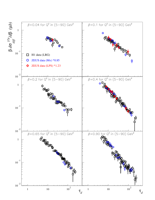
Figure 2: The diffractive cross section $\beta\ d\sigma^{\gamma^{*}p\rightarrow Xp}_{diff}/d\beta$ from H1 and ZEUS measurements, as a function of $\tau_{d}$ in bins of $\beta$ for $Q^{2}$ values in the range $[5;90]\ \mbox{GeV}^{2}$ and for $x_{\rm l\!P}\!<\!0.01.$ Only statistical uncertainties are shown.

Let us finally confront the prediction (22) with DVCS and vector-meson production data from HERA. On Fig.3, the available measurements from H1 and ZEUS for DVCS dvcs , $\rho$ rho , $\phi$ phi and $J/\psi$ jpsi exclusive productions are displayed. We represent the total cross-sections (meaning $t$-integrated) as a function of $\tau_{V}$ ($\tau_{V}\!=\!\tau$ for DVCS) with the saturation scale (15). Again, for each vector meson, the data lie on a single curve, confirming the geometric scaling prediction.

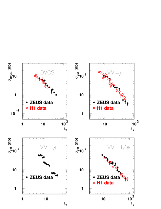
Figure 3: The $\rho$, $J/\Psi$ and $\phi$ production cross-sections $\sigma^{\gamma^{*}p\rightarrow Vp}_{VM}$ and the DVCS cross-section $\sigma^{\gamma^{*}p\rightarrow\gamma p}_{DVCS}$ from H1 and ZEUS measurements, as a function of $\tau_{V}$ and for $x_{\rm l\!P}\!<\!0.01.$ Only statistical uncertainties are shown.

V Conclusions

The dipole picture of deep inelastic scattering is a theoretical framework provided by perturbative QCD ($Q^{2}\!\gg\!\Lambda_{QCD}^{2}$) in the high-energy limit ($x\!\ll\!1$). It allows to express total (6), diffractive (7) and exclusive (10) cross-sections in terms of a single object: a dipole scattering amplitude off the proton. One of the main features of the saturation regime of QCD is the scaling law (12) of this dipole amplitude. The resulting consequence, the geometric scaling (14) of the total cross-section in DIS, is well-known and geometric scaling has been found in the data five years ago geoscal . As shown in Fig.1, the present data confirm it.

In this letter, we have exhibited the consequences of the scaling (12) for diffractive observables in DIS, namely for the diffractive cross-section (7) and the vector-meson production (and DVCS) cross-section (10). We have shown that further manifestations of the saturation scale should appear in the diffractive data in the form of the scaling laws (18) and (22) with the same saturation scale $Q_{s}$ as in the inclusive case (14). We have analysed the present data and shown them in Fig.2 and Fig.3. These confirm the expected behaviors and suggest that all three scaling displayed in Fig.1, Fig.2 and Fig.3 are indeed manifestations of the saturation regime of QCD.

For the saturation scale $Q_{s},$ we have taken over the same values of the parameters $\lambda$ and $x_{0}$ as in golec . We did not try to vary them to obtain a better scaling. In the context of the exact scaling law (12), a definite value for those parameters does not really make sense anyway. Indeed, fits of different QCD-inspired saturation models golec ; satmod on $\sigma^{\gamma^{*}p\rightarrow X}_{tot}(x,Q^{2})$ have shown that the precise values of the parameter are sensitive to whether or not scaling violations are included (they are also sensitive to what type of scaling violations are included). In any case, the parameters never differ significantly from those we used here.

Note finally that in the case of vector-meson production, we only looked at cross-sections integrated over the momentum transfer $t.$ Cross-sections differential with respect to $t$ can also be expressed in the dipole picture, with the $t$ dependence of the cross-section related to the impact parameter dependence of the dipole amplitude via a Fourier transform (see for instance mms ; kowtea ). We did not consider such observables in this work, but they represent natural places to look for geometric scaling properties at non-zero transfer as was predicted in nfgs . It would require to carry out measurements with broad ranges for the $x$ and $Q^{2}$ values (i.e. a large range for $\tau$), for different fixed values of $t.$ This may be an experimental challenge, but it would certainly be worthy. It would especially help our understanding of the impact parameter (b) dependence of the dipole amplitude, and our understanding of how it is mixed with the high-energy evolution.

- (1) L.V. Gribov, E.M. Levin and M.G. Ryskin, Phys. Rep. 100 (1983) 1.
- (2) E. Iancu, K. Itakura and L. McLerran, Nucl. Phys. A708 (2002) 327.
- (3) A.M. Staśto, K. Golec-Biernat and J. Kwiecinski, Phys. Rev. Lett. 86 (2001) 596.
- (4) K. Golec-Biernat and M. Wüsthoff, Phys. Rev. D59 (1999) 014017; Phys. Rev. D60 (1999) 114023.
- (5) A.H. Mueller, Nucl. Phys. B335 (1990) 115; N.N. Nikolaev and B.G. Zakharov, Zeit. für. Phys. C49 (1991) 607.
- (6) N.N. Nikolaev and B.G. Zakharov, Zeit. für. Phys. C53 (1992) 331.
- (7) A. Bialas and R. Peschanski, Phys. Lett. B378 (1996) 302; Phys. Lett. B387 (1996) 405; A. Bialas, R. Peschanski and C. Royon, Phys. Rev. D57 (1998) 6899; S. Munier, R. Peschanski and C. Royon, Nucl. Phys. B534 (1998) 297.
- (8) E. Iancu, Y. Hatta, C. Marquet, G. Soyez and D.N. Triantafyllopoulos, Nucl. Phys. A773 (2006) 95.
- (9) J. Bartels, H. Jung and M. Wüsthoff, Eur. Phys. J. C11 (1999) 111.
- (10) B.Z. Kopeliovich, A. Schaefer and A.V. Tarasov, Phys. Rev. D62 (2000) 054022.
- (11) Yu.V. Kovchegov, Phys. Rev. D64 (2001) 114016.
- (12) S. Munier and A. Shoshi, Phys. Rev. D69 (2004) 074022.
- (13) C. Marquet, Nucl. Phys. B705 (2005) 319; Nucl. Phys. A755 (2005) 603c; K. Golec-Biernat and C. Marquet, Phys. Rev. D71 (2005) 114005.
- (14) M. Wüsthoff, Phys. Rev. D56 (1997) 4311.
- (15) J. Nemchik, N.N. Nikolaev and B.G. Zakharov, Phys. Lett. B341 (1994) 228; J. Nemchik, N.N. Nikolaev, E. Predazzi and B.G. Zakharov, Zeit. für. Phys. C75 (1997) 71.
- (16) L. Frankfurt, W. Koepf and M. Strikman, Phys. Rev. D54 (1996) 3194.
- (17) H.G. Dosch, T. Gousset, G. Kulzinger and H.J. Pirner, Phys. Rev. D55 (1997) 2602; G. Kulzinger, H.G. Dosch and H.J. Pirner, Eur. Phys. J. C7 (1999) 73.
- (18) I. Balitsky, Nucl. Phys. B463 (1996) 99; Phys. Lett. B518 (2001) 235; Yu.V. Kovchegov, Phys. Rev. D60 (1999) 034008; Phys. Rev. D61 (2000) 074018.
- (19) J. Jalilian-Marian, A. Kovner, A. Leonidov and H. Weigert, Nucl. Phys. B504 (1997) 415; Phys. Rev. D59 (1999) 014014; J. Jalilian-Marian, A. Kovner and H. Weigert, Phys. Rev. D59 (1999) 014015; E. Iancu, A. Leonidov and L. McLerran, Nucl. Phys. A692 (2001) 583; Phys. Lett. B510 (2001) 133; E. Ferreiro, E. Iancu, A. Leonidov and L. McLerran, Nucl. Phys. A703 (2002) 489; H. Weigert, Nucl. Phys. A703 (2002) 823.
- (20) S. Munier and R. Peschanski, Phys. Rev. Lett. 91 (2003) 232001; Phys. Rev. D69 (2004) 034008; Phys. Rev. D70 (2004) 077503.
- (21) A.H. Mueller and A.I Shoshi, Nucl. Phys. B692 (2004) 175; E. Iancu, A.H. Mueller and S. Munier, Phys. Lett. B606 (2005) 342; A.H. Mueller, A.I Shoshi and S.M.H. Wong, Nucl. Phys. B715 (2005) 440; E. Iancu and D. Triantafyllopoulos, Nucl. Phys. A756 (2005) 419; Phys. Lett. B610 (2005) 253.
- (22) D. Schildknecht, B. Surrow and M. Tentyukov, Phys. Lett. B499 (2001) 116; Mod. Phys. Lett. A16 (2001) 1829.
- (23) C. Adloff et al. [H1 Collaboration], Eur. Phys. J. C21 (2001) 33.
- (24) J. Breitweg et al. [ZEUS Collaboration], Phys. Lett. B487 (2000) 53; S. Chekanov et al. [ZEUS Collaboration], Eur. Phys. J C21 (2001) 443.
- (25) M.R. Adams et al. [E665 Collaboration], Phys. Rev. D54 (1996) 3006.
- (26) M. Arneodo et al. [NMC Collaboration], Nucl. Phys. B483 (1997) 3.
- (27) V.P. Goncalves and M.V.T. Machado, Phys. Rev. Lett. 91 (2003) 202002.
- (28) S. Munier, A.M. Stasto and A.H. Mueller, Nucl. Phys. B603 (2001) 427.
- (29) A. Aktas et al. [H1 Collaboration], “Measurement and QCD Analysis of the Diffractive Deep-Inelastic Scattering Cross Section at HERA”, arXiv:hep-ex/0606004.
- (30) S. Chekanov et al. [ZEUS Collaboration], Nucl. Phys. B713 (2005) 3.
- (31) S. Chekanov et al. [ZEUS Collaboration], Eur. Phys. J. C38 (2004) 43.
- (32) A. Aktas et al. [H1 Collaboration], Eur. Phys. J. C44 (2005) 1; S. Chekanov et al. [ZEUS Collaboration], Phys. Lett. B573 (2003) 46.
- (33) C. Adloff et al. [H1 Collaboration], Eur. Phys. J. C13 (2000) 371; J. Breitweg et al. [ZEUS Collaboration], Eur. Phys. J. C6 (1999) 603.
- (34) S. Chekanov et al. [ZEUS Collaboration], Nucl. Phys. B718 (2005) 3.
- (35) A. Aktas et al. [H1 Collaboration], “Elastic J/Psi Production at HERA”, arXiv:hep-ex/0510016; S. Chekanov et al. [ZEUS Collaboration], Nucl. Phys. B695 (2004) 3.
- (36) E. Iancu, K. Itakura and S. Munier, Phys. Lett. B590 (2004) 199; J. Bartels, K. Golec-Biernat and H. Kowalski, Phys. Rev. D66 (2002) 0114001.
- (37) S. Munier and S. Wallon, Eur. Phys. J. C30 (2003) 359; H. Kowalski and D. Teaney, Phys. Rev. D68 (2003) 114005.
- (38) C. Marquet, R. Peschanski and G. Soyez, Nucl. Phys. A756 (2005) 399; C. Marquet and G. Soyez, Nucl. Phys. A760 (2005) 208.