Abstract

In many extensions of the Standard Model, including a broad class of left-right symmetric and Grand Unified theories, the light neutrino mass matrix is given by the left-right symmetric seesaw formula $M_{\nu}=fv_{L}-\frac{v^{2}}{v_{R}}Y_{\nu}f^{-1}Y_{\nu}$, in which the right-handed neutrino mass matrix and the $SU(2)_{L}$ triplet couplings are proportional to the same matrix $f$. We propose a systematic procedure for reconstructing the $2^{n}$ solutions (in the $n$-family case) for the matrix $f$ as a function of the Dirac neutrino couplings $(Y_{\nu})_{ij}$ and of the light neutrino mass parameters, which can be used in both analytical and numerical studies. We apply this procedure to a particular class of supersymmetric $SO(10)$ models with two $\bf 10$-dimensional and a pair of $\bf 126\oplus\overline{126}$ representations in the Higgs sector, and study the properties of the corresponding 8 right-handed neutrino spectra. Then, using the reconstructed right-handed neutrino and triplet parameters, we study leptogenesis and lepton flavour violation in these models, and comment on flavour effects in leptogenesis in the type I limit. We find that the mixed solutions where both the type I and the type II seesaw mechanisms give a significant contribution to neutrino masses provide new opportunities for successful leptogenesis in $SO(10)$ GUTs.

1 Introduction

Experimental data suggest that neutrinos are massive and mix. The most popular explanation of the smallness of their masses relies on the (type I) seesaw mechanism [1], which finds a natural realization in Grand Unified Theories (GUTs) based on the $SO(10)$ gauge group. While the seesaw mechanism cannot be directly tested since, at least in its GUT version, it involves superheavy states, it has observable consequences: leptogenesis [2] and, in supersymmetric theories, flavour [3] and CP violation [4] in the lepton sector. Successful leptogenesis puts several constraints on the seesaw parameters [5, 6, 7]; in particular, the mass of the lightest right-handed neutrino, $M_{1}$, should be larger than ${\cal O}(10^{8}-10^{9})$ GeV in the case of a hierarchical mass spectrum. It is well-known that in $SO(10)$ models where the dominant contribution to fermion masses comes from 10-dimensional Higgs representations, the right-handed neutrino mass spectrum reconstructed from the type I seesaw mass formula is strongly hierarchical (except for special values of the light neutrino mass parameters [8]), with $M_{1}$ lying below the minimal value for a successful leptogenesis [9].

However, many extensions of the Standard Model contain two sources for neutrino masses and leptogenesis: the type I (associated with the exchange of right-handed neutrinos) [1] and type II (associated with the exchange of heavy scalar $SU(2)_{L}$ triplets) [10, 11] (see also Ref. [12]) seesaw mechanisms. In particular, in a broad class of left-right symmetric and Grand Unified theories, the light neutrino mass matrix is given by the left-right symmetric seesaw formula $M_{\nu}=fv_{L}-\frac{v^{2}}{v_{R}}Y_{\nu}f^{-1}Y_{\nu}$, in which the right-handed neutrino mass matrix and the heavy triplet couplings are proportional to the same matrix $f$. Very often in the literature it is assumed that either of these two mechanisms dominates in the neutrino mass matrix. But, as discussed below, this corresponds to assuming specific values of the unknown seesaw parameters. In a general study one should encompass the situation where both contributions are sizeable and can be comparable in magnitude. In order to implement in an efficient way our experimental knowledge about neutrino masses and mixings, we need a procedure to reconstruct the matrix $f$ as a function of the Dirac neutrino couplings. This problem has been first addressed in Ref. [13], where it was found that there are exactly $2^{n}$ different solutions in the n-family case, which are connected two by two by a transformation called “seesaw duality”.

In this paper, we use a different, more efficient procedure to reconstruct the $2^{n}$ solutions, which employs complex orthogonal transformations and is appropriate to both numerical and analytic studies. For three generations of neutrinos, the eight solutions correspond to the different combinations of the roots of three quadratic equations. We apply this procedure to a particular class of supersymmetric $SO(10)$ models with two $\bf 10$-dimensional and a pair of $\bf 126\oplus\overline{126}$ representations in the Higgs sector, and use the results to study leptogenesis and lepton flavour violation in these models. The spectrum of possibilities to account for the observed neutrino data is much richer than in the cases of type I and type II dominance, and the mixed solutions where both seesaw mechanisms give a significant contribution to neutrino masses provide new opportunities for successful leptogenesis in $SO(10)$ GUTs.

The content of the paper is as follows. In Section 2, we present the procedure for reconstructing the $2^{n}$ solutions for the matrix $f$ from the light neutrino mass parameters, assuming that the Dirac matrix is known, and we discuss the properties of the solutions. In section 3, we apply the procedure to supersymmetric $SO(10)$ models with two $\bf 10$-dimensional and a pair of $\bf 126\oplus\overline{126}$ representations in the Higgs sector, and display the corresponding 8 right-handed neutrino spectra as a function of the $B-L$ breaking scale, for various values of the free parameters (which include several phases). In Section 4, we compute the CP asymmetry in right-handed neutrino decays for the 8 solutions, and comment on flavour effects in the type I limit. In Section 5, we discuss the predictions for lepton flavour violating processes. Finally, in Section 6, we give our conclusions and comment on possible extensions of the present work. Analytic approximations that can be useful to understand the results of the reconstruction procedure are given in Appendix B.

2 Reconstruction of the heavy neutrino mass spectrum

In many extensions of the Standard Model based on a gauge group embedding the left-right symmetric group $SU(2)_{L}\times SU(2)_{R}\times U(1)_{B-L}$, the neutrino mass matrix is given by the following seesaw formula [10, 11]:

$$M_{\nu}\ =\ f_{L}v_{L}-\frac{v^{2}}{v_{R}}Y^{T}_{\nu}f^{-1}_{R}Y_{\nu}\ ,$$ (1)

where $f_{L}$ and $f_{R}$ are symmetric matrices. The second term in the right-hand side of Eq. (1) is the usual type I seesaw mass term, where the heavy Majorana mass matrix $M_{R}=f_{R}v_{R}$ is generated from the vev of an $SU(2)_{R}$ triplet $\Delta_{R}$ with couplings $(f_{R})_{ij}$ to right-handed neutrinos, and $M_{D}=Y_{\nu}v$ is the Dirac mass matrix ($v=174$ GeV is the vev of the SM Higgs doublet, to be replaced by $v_{u}=v\sin\beta$ in supersymmetric models). The first term, known as the type II seesaw mass term, is generated from the exchange of an heavy $SU(2)_{L}$ triplet $\Delta_{L}$ with couplings $(f_{L})_{ij}$ to lepton doublets. The induced vev $v_{L}$ is related to the heavy triplet mass $M_{\Delta_{L}}$ by $v_{L}\sim v^{2}v_{R}/M^{2}_{\Delta_{L}}$, which naturally explains its smallness.

In this paper, we consider theories in which the couplings of the $SU(2)_{L}$ and $SU(2)_{R}$ triplets are equal and the Dirac mass matrix is symmetric, so that Eq. (1) becomes:

$$M_{\nu}\ =\ fv_{L}-\frac{v^{2}}{v_{R}}Y_{\nu}f^{-1}Y_{\nu}\ .$$ (2)

These relations arise naturally in $SO(10)$ GUTs in which the right-handed neutrino masses are generated from a $\bf\overline{126}$ Higgs representation [10] (barring non-symmetric contributions to the Yukawa couplings, coming e.g. from a $\bf 120$ Higgs representation), as well as in a broad class of left-right symmetric theories [11].

2.1 Reconstruction procedure

Our starting point is the left-right symmetric seesaw formula (2), where both $f$ and $Y_{\nu}$ are complex symmetric matrices. Our goal is to determine the matrix $f$ for a given pattern of light neutrino masses and mixings, assuming that the Dirac matrix $Y_{\nu}$ is known in a basis in which the charged lepton mass matrix is diagonal. For definiteness we work in the $3$-family case, but the procedure applies to any number of neutrino families.

If $Y_{\nu}$ is invertible, Eq. (2) can be rewritten in the form:

$$Z\ =\ \alpha X-\beta X^{-1}\ ,$$ (3)

with $\alpha\equiv v_{L}/m_{\nu}$, $\beta\equiv v^{2}/(m_{\nu}v_{R})$ and

$$Z\ \equiv\ \frac{1}{m_{\nu}}\ Y_{\nu}^{-1/2}M_{\nu}(Y_{\nu}^{-1/2})^{T}\ ,\qquad X\ \equiv\ Y_{\nu}^{-1/2}f(Y_{\nu}^{-1/2})^{T}\ ,$$ (4)

where $Y_{\nu}^{1/2}$ is a matrix such that $Y_{\nu}=Y_{\nu}^{1/2}(Y_{\nu}^{1/2})^{T}$ (in order to deal with dimensionless quantities, we have introduced a mass scale $m_{\nu}$ characteristic of the light neutrino mass spectrum). Since $Y_{\nu}$ is assumed to be known in the basis of charged lepton mass eigenstates, the matrix $Z$ is completely determined (up to possible high-energy phases) by the choice of the light neutrino mass and mixing pattern.

Assuming further that the polynomial equation $\det(Z-z\mathbf{1})=0$ has three distinct roots $z_{1,2,3}$, we can diagonalize the complex symmetric matrix $Z$ with a complex orthogonal matrix:

$$Z\ =\ O_{Z}\mbox{Diag}\,(z_{1},z_{2},z_{3})O^{T}_{Z}\ ,\qquad O_{Z}O^{T}_{Z}\ =\ \mathbf{1}\ ,$$ (5)

where the $z_{i}$ are complex numbers. Then Eq. (3) can be solved for $X$ in a straightforward manner, by noting that $X$ is diagonalized by the same complex orthogonal matrix as $Z$:

$$X\ =\ O_{Z}\mbox{Diag}\,(x_{1},x_{2},x_{3})O^{T}_{Z}\ ,$$ (6)

with the $x_{i}$ being the solutions of the quadratic equation $z_{i}=\alpha x_{i}-\beta x^{-1}_{i}$. For a given choice of ($x_{1}$, $x_{2}$, $x_{3}$), the matrix $f$ is given by:

$$f\ =\ Y_{\nu}^{1/2}X(Y_{\nu}^{1/2})^{T}\ =\ Y_{\nu}^{1/2}\,O_{Z}\,\mbox{Diag}\,(x_{1},x_{2},x_{3})\,O^{T}_{Z}\,(Y_{\nu}^{1/2})^{T}\ ,$$ (7)

and the right-handed neutrino masses $M_{i}=f_{i}v_{R}$ are obtained by diagonalizing $f$ with a unitary matrix:

$$f\ =\ U_{f}\hat{f}U^{T}_{f}\ ,\qquad\hat{f}\ =\ \mbox{Diag}\,(f_{1},f_{2},f_{3})\ ,\qquad U_{f}U^{\dagger}_{f}=\mathbf{1}\ ,$$ (8)

where the $f_{i}$ are chosen to be real and positive. The matrix $U_{f}$ relates the original basis for right-handed neutrinos, in which $Y_{\nu}$ is symmetric, to their mass eigenstate basis. It can be used to express the Dirac couplings in terms of charged lepton and right-handed neutrino mass eigenstates, as $Y\equiv U^{\dagger}_{f}Y_{\nu}$.

Since there are two possible choices for each $x_{i}$, we have 8 different solutions for the matrix $f$ ($2^{n}$ in the $n$-generation case), a property already found in Ref. [13]. The advantage of the above procedure over the one presented in Ref. [13] is that it is more systematic and allows for an easier reconstruction of the right-handed neutrino masses and mixings, both analytically and numerically. Furthermore, the connection between the different solutions is more transparent.

2.2 Properties of the 8 solutions

In order to label the 8 different solutions for $f$, we denote the two solutions of the equation $z_{i}=\alpha x_{i}-\beta x^{-1}_{i}$ by $x^{+}_{i}$ and $x^{-}_{i}$, with

$$x^{\pm}_{i}\ \equiv\ \frac{z_{i}\pm\mbox{sign}(\mbox{Re}(z_{i}))\sqrt{z^{2}_{i}+4\alpha\beta}}{2\alpha}\ .$$ (9)

With the above definition, one has, in the limit where $4\alpha\beta\ll|z_{i}|^{2}\,$:

$$x^{+}_{i}\ \simeq\ \frac{z_{i}}{\alpha}\ ,\qquad x^{-}_{i}\ \simeq\ -\frac{\beta}{z_{i}}\ ,$$ (10)

while in the limit $|z_{i}|^{2}\ll 4\alpha\beta$:

$$x^{\pm}_{i}\ \simeq\ \pm\,\mbox{sign}(\mbox{Re}(z_{i}))\sqrt{\beta/\alpha}\ .$$ (11)

We label the 8 solutions for $f$ in the following way: $(+,+,+)$ refers to the solution $(x^{+}_{1},x^{+}_{2},x^{+}_{3})$, $(+,+,-)$ to the solution $(x^{+}_{1},x^{+}_{2},x^{-}_{3})$, and so on. We will sometimes refer to $x^{-}_{i}$ as the “type I branch” and to $x^{+}_{i}$ as the “type II branch”, for reasons that will become clear below.

For some particular solutions, Eq. (10) has an immediate interpretation in terms of dominance of the type I or type II contribution to light neutrino masses. More precisely, for values of $\alpha\beta$ such that $4\alpha\beta\ll|z_{1}|^{2}$, the solutions $(+,+,+)$ and $(-,-,-)$ practically coincide with the “pure” type II and type I cases, respectively. Indeed, plugging the approximate relations $X^{(+,+,+)}\simeq Z/\alpha$ and $X^{(-,-,-)}\simeq-\beta Z^{-1}$ into Eqs. (4), one obtains:

$$f^{(+,+,+)} \stackrel{{\scriptstyle 4\alpha\beta\ll|z_{1}|^{2}}}{{\longrightarrow}} \frac{M_{\nu}}{v_{L}}\qquad\qquad\qquad\ \ \mbox{(type II limit)}\ ,$$ (12)

$$f^{(-,-,-)} \stackrel{{\scriptstyle 4\alpha\beta\ll|z_{1}|^{2}}}{{\longrightarrow}} -\,\frac{v^{2}}{v_{R}}\,Y_{\nu}M^{-1}_{\nu}Y_{\nu}\qquad\mbox{(type I limit)}\ .$$ (13)

The remaining 6 solutions correspond to mixed cases where, even in the $4\alpha\beta\ll|z_{1}|^{2}$ limit, the light neutrino mass matrix receives significant contributions from both types of seesaw mechanisms. Depending on the Dirac couplings as well as on the light neutrino mass and mixing pattern, one may have solutions where e.g. the type I contribution dominates in some entries of the light neutrino mass matrix, while both seesaw mechanisms contribute to the other entries.

There is another range of values for $\alpha\beta$ in which $f$ reaches a remarkable limit, namely $|z_{3}|^{2}\ll 4\alpha\beta$. In this region, one has $x^{\pm}_{i}\simeq\pm\mbox{sign}(\mbox{Re}(z_{i}))\sqrt{\beta/\alpha}$ for all $i$, which indicates a strong cancellation between the type I and type II contributions to the light neutrino mass matrix. This can easily be seen for the two solutions labelled by $(\pm\epsilon_{1},\pm\epsilon_{2},\pm\epsilon_{3})$, $\epsilon_{i}\equiv\mbox{sign}(\mbox{Re}(z_{i}))$, in which one has $X\simeq\pm\sqrt{\beta/\alpha}\,{\bf 1}$. Using Eqs. (4), this leads to:

$$f^{(\pm\epsilon_{1},\pm\epsilon_{2},\pm\epsilon_{3})}\ \stackrel{{\scriptstyle 4\alpha\beta\gg|z_{3}|^{2}}}{{\longrightarrow}}\ \pm\sqrt{\beta/\alpha}\,Y_{\nu}\ ,$$ (14)

which shows that the type I and type II contributions approximately cancel in $M_{\nu}$. For the other 6 solutions, Eq. (14) does not hold but one still has $f_{i}\simeq\sqrt{\beta/\alpha}\,y_{i}$ (where the $y_{i}$ are the eigenvalues of $Y_{\nu}$) in the $|z_{3}|^{2}\ll 4\alpha\beta$ regime, provided that the Dirac matrix has a hierarchical structure. Moreover, for the type of hierarchy considered in Section 3, one can show that $f\simeq\sqrt{\beta/\alpha}\,U^{T}_{\nu}\mbox{Diag}\,(s_{1}y_{1},s_{2}y_{2},s_{3}y_{3})U_{\nu}$ in the $|z_{3}|^{2}\ll 4\alpha\beta$ regime, where $Y_{\nu}=U^{T}_{\nu}\mbox{Diag}\,(y_{1},y_{2},y_{3})U_{\nu}$ and $s_{i}=\pm\,\mbox{sign}(\mbox{Re}(z_{i}))$ for $x_{i}=x^{\pm}_{i}$ (see Appendix B).

Finally, in the intermediate region of values for $\alpha\beta$, $|z_{1}|^{2}<4\alpha\beta<|z_{3}|^{2}$, both the type I and the type II seesaw mechanism give significant contributions to the light neutrino mass matrix. Already for $|z_{1}|^{2}\ll 4\alpha\beta$, cancellations between the right-handed neutrino and triplet contributions to $M_{\nu}$ start to occur.

The 8 different solutions for $f$ are connected to each other by the three transformations:

$$x_{i}\ \rightarrow\ \tilde{x}_{i}\equiv z_{i}/\alpha-x_{i}\ ,$$ (15)

which act as $x^{+}_{i}\leftrightarrow x^{-}_{i}$. This generalizes the “seesaw duality” of Ref. [13], defined as $f\rightarrow\tilde{f}\equiv M_{\nu}/v_{L}-f$, which amounts to interchange the type I and type II branches for all three $x_{i}$ simultaneously, thus dividing the 8 solutions into 4 “dual pairs”. The transformations (15), more generally, allow to generate all 8 solutions from a single one. In group-theoretical terms, these transformations define an abelian group $Z_{2}\otimes Z_{2}\otimes Z_{2}$ of 8 elements, one of which is the “seesaw duality” of Ref. [13].

3 A case study: right-handed neutrinos in $SO(10)$ models

The procedure described in Subsection 2.1 can be used to determine the a priori unknown $f_{ij}$ couplings in theories which predict the Dirac matrix $Y_{\nu}$, taking low-energy neutrino data as an input. In the following, we apply it to reconstruct the right-handed neutrino mass spectrum in a class of supersymmetric $SO(10)$ models with two $\bf 10$-dimensional and a pair of $\bf 126\oplus\overline{126}$ representations in the Higgs sector.

3.1 Input parameters

In supersymmetric $SO(10)$ models with two $\bf 10$-dimensional and a pair of $\bf 126\oplus\overline{126}$ representations (but no $\bf 120$-dimensional representation) in the Higgs sector, the most general Yukawa couplings read:

$$Y^{(1)}_{ij}\,{\bf 16_{i}}{\bf 16_{j}}{\bf 10_{1}}+Y^{(2)}_{ij}\,{\bf 16_{i}}{\bf 16_{j}}{\bf 10_{2}}+f_{ij}\,{\bf 16_{i}}{\bf 16_{j}}{\bf\overline{126}}\ ,$$ (16)

where $Y^{(1)}$, $Y^{(2)}$ and $f$ are complex symmetric matrices. Assuming that the $SU(2)_{L}$ doublet components of the $\bf\overline{126}$ do not acquire a vev, Eq. (16) leads to the following mass relations for the charged fermions, valid at the GUT scale:

$$M_{u}\ =\ M_{D}\ ,\qquad M_{d}\ =\ M_{e}\ .$$ (17)

It is well-known that the second relation is in conflict with experimental data and needs to be corrected. In general, the corrections (coming e.g. from the $SU(2)_{L}$ doublet components in the $\bf\overline{126}$ [16], or from non-renormalizable operators [17]) also affect the first relation. Although these corrections will change numerically the solutions for $f$, we do not expect them to alter the qualitative features of our results. As a case study, we assume Eq. (17) to hold in the following.

The inputs in the procedure for reconstructing the 8 solutions for $f$ are the matrices $Y_{\nu}$ and $M_{\nu}$ at the seesaw scale. The “boundary condition” for $Y_{\nu}$, Eq. (17), is defined at the GUT scale, where it is convenient to work in the basis for the $\bf 16$ matter representations in which $M_{e}$ (hence $M_{d}$) is diagonal with real positive entries. In this basis, the Dirac matrix reads:

$$Y_{\nu}\ =\ U^{T}_{q}\hat{Y}_{u}U_{q}\ ,\qquad U_{q}\ =\ P_{u}V_{CKM}P_{d}\ ,\qquad\hat{Y}_{u}\ =\ \mbox{Diag}\,(y_{u},y_{c},y_{t})\ ,$$ (18)

where $V_{CKM}$ is the CKM matrix and $y_{u,c,t}$ are the up quark Yukawa couplings, all renormalized at the GUT scale. The presence of two diagonal matrices of phases $P_{u}$ and $P_{d}$ in Eq. (18) is due to the fact that the $SO(10)$ symmetry prevents independent rephasing of right-handed and left-handed quark fields. Since $Y_{\nu}$ is only weakly renormalized between $M_{GUT}$ and the seesaw scale, the effet of the running being smaller than the uncertainty on the quark parameters at $M_{GUT}$, we can neglect it and assume Eq. (18) to hold at the seesaw scale, in the basis of charged lepton mass eigenstates. In the same basis, the light neutrino mass matrix generated from the seesaw mechanism reads:

$$M_{\nu}\ =\ U^{\star}_{l}\hat{M}_{\nu}U^{\dagger}_{l}\ ,\qquad U_{l}\ =\ P_{e}U_{PMNS}P_{\nu}\ ,\qquad\hat{M}_{\nu}\ =\ \mbox{Diag}\,(m_{1},m_{2},m_{3})\ ,$$ (19)

where $U_{PMNS}$ is the PMNS matrix and $m_{1,2,3}$ are the light neutrino masses, all renormalized at the seesaw scale. The two relative phases in $P_{\nu}$ are the physical CP-violating phases associated with the Majorana nature of the light neutrinos, while the three phases contained in $P_{e}$, analogous to the five independent phases contained in $P_{u}$ and $P_{d}$, are pure high-energy phases. Having specified Eqs. (18) and (19), one can apply the procedure presented in Subsection 2.1 and reconstruct the 8 different matrices $f$ corresponding to a given light neutrino mass and mixing pattern as a function of $\alpha$, $\beta$ and of the high-energy phases contained in $P_{u}$, $P_{d}$ and $P_{e}$.

The associated right-handed neutrino mass and mixing patterns strongly depend on the values of $\alpha$ and $\beta$ (or equivalently $\beta/\alpha$ and $v_{R}$), which in turn depend on the details of the model. The simplest way to realize the type II seesaw mechanism in the class of $SO(10)$ models considered is to introduce a $\bf 54$ representation in the Higgs sector in addition to the $\bf\overline{126}\oplus 126$ pair. This is easily seen in a left-right symmetric language: the $\bf\overline{126}$ contains a right-handed triplet $\Delta^{c}$ with quantum numbers ${\bf(1,3,1)_{-2}}$ under $SU(2)_{L}\times SU(2)_{R}\times SU(3)_{C}\times U(1)_{B-L}$, whose vev $v_{R}$ is responsible for the breaking of $B-L$, as well as a left-handed triplet $\Delta={\bf(3,1,1)_{+2}}$; the $\bf 54$ contains a bitriplet $\tilde{\Delta}={\bf(3,3,1)_{0}}$; and each $\bf 10$ contains a bidoublet $\Phi={\bf(2,2,1)_{0}}$. The superpotential terms relevant for the type II contribution to neutrino masses include:

$$W\ =\ \frac{1}{2}\,f_{ij}\,L_{i}L_{j}\Delta+\kappa\,\Phi\Phi\tilde{\Delta}+\lambda\,\Delta\Delta^{c}\tilde{\Delta}+\ \ldots\ ,$$ (20)

where the first term comes from the ${\bf 16_{i}}{\bf 16_{j}}{\bf\overline{126}}$ couplings, and the second and third terms come from the $\bf 10\,10\,54$ and $\bf 54\,\overline{126}\,\overline{126}$ couplings, respectively. The presence of these terms induces a vev $v_{L}\sim\kappa\lambda v^{2}_{u}v_{R}/M^{2}_{\Delta_{L}}$ for the $SU(2)_{L}$ triplet, yielding a ratio $\beta/\alpha=v^{2}_{u}/(v_{L}v_{R})\sim M^{2}_{\Delta_{L}}/(\kappa\lambda v^{2}_{R})$. Depending on the other superpotential couplings, the triplet mass $M_{\Delta_{L}}$ may be larger or smaller than $v_{R}$ (for $v_{R}\ll M_{GUT}$, a tuning of the superpotential parameters might be necessary to achieve $M_{\Delta_{L}}<v_{R}$), hence $\beta/\alpha$ can be larger or smaller than $1$. As for $v_{R}$, its value is related to the breaking scheme of the GUT symmetry and is also model dependent. In principle the $B-L$ symmetry could be broken anywhere between the Planck scale and the weak scale; however the requirement of gauge coupling unification generically disfavours the breaking of $B-L$ at lower scales. Detailed studies (see e.g. Ref. [19]) have shown that the $B-L$ symmetry can be broken a few orders of magnitude below the GUT scale consistently with unification. In the following, we allow $v_{R}$ to vary in the range $(10^{12}-10^{17})$ GeV.

3.2 Right-handed neutrino spectra

In this subsection, we display the right-handed neutrino spectra obtained from the reconstruction of the couplings $f_{ij}$ in the class of $SO(10)$ models specified above. For definiteness, we consider the case of a hierarchical light neutrino mass spectrum with $m_{1}=10^{-3}$ eV, and we take the best fit values of Ref. [20] for the oscillation parameters (the parametrization of the PMNS matrix is the one adopted in the Review of Particle Properties [21]):

$$\Delta m^{2}_{32}\equiv m^{2}_{3}-m^{2}_{2}=2.4\times 10^{-3}\,\mbox{eV}^{2},\qquad\Delta m^{2}_{21}\equiv m^{2}_{2}-m^{2}_{1}=7.92\times 10^{-5}\,\mbox{eV}^{2},$$ (21)

$$\sin^{2}\theta_{23}=0.44\ ,\qquad\sin^{2}\theta_{12}=0.314\ ,\qquad\sin^{2}\theta_{13}=0.009\ .$$ (22)

The PMNS phase $\delta$ and the two relative Majorana phases contained in $P_{\nu}$ are treated as free parameters in our study, like the high-energy phases contained in $P_{u}$, $P_{d}$ and $P_{e}$. The renormalization group running between low energy and the seesaw scale has little impact on the neutrino parameters in the case of a hierarchical spectrum, apart from an overall scaling of the light neutrino masses [22] which we roughly take into account by multiplying their low-energy values by a factor $1.2$ [23].

In the quark sector, we take into account the renormalization group running by setting $A(M_{GUT})=0.7$ in the Wolfenstein parametrization of the CKM matrix, and $\hat{Y}_{u}(M_{GUT})=\mbox{Diag}\,(6\times 10^{-6},2.5\times 10^{-3},1)\times y_{t}(M_{GUT})$, with $y_{t}(M_{GUT})=0.7$. In our estimate of the GUT-scale values for the up quark Yukawa couplings, we have taken the central values for the first and second generation quark masses given in the Review of Particle Properties [21]. Furthermore, we take $\lambda=0.22$, $\rho=0.2$ and $\eta=0.35$, in agreement with fits of the unitary triangle [24].

Before presenting the 8 right-handed neutrino spectra corresponding to these inputs, let us mention the restrictions that apply to the reconstructed couplings $f_{ij}$. A first restriction comes from the requirement of perturbativity, i.e. the $f_{ij}$’s should remain in the perturbative regime up to the scale at which the unified gauge coupling $g_{10}$ blows up, $\Lambda_{10}\approx 2\times 10^{17}$ GeV. As discussed in Appendix A, we can safely take $f_{3}<1$ as a perturbativity constraint at the seesaw scale where the $f_{ij}$’s are determined. One can impose a second restriction on the couplings $f_{ij}$ by requiring that there be no unnatural cancellations between the type I and the type II contributions to neutrino masses. In practice, we shall define the fine-tuned region by:

$$f_{33}\,v_{L}\ >\ F(M_{\nu})_{33}\ ,$$ (23)

where $F$ measures the level of fine-tuning in the $(3,3)$ entry of the light neutrino mass matrix: $F=10$ corrresponds to a $10\%$ fine-tuning, and so on. Such cancellations might be the consequence of a symmetry ensuring a proportionality relation between $f$ and $Y_{\nu}$, and are not necessarily unnatural. Nevertheless a high degree of fine-tuning would be unstable against radiative corrections, since this symmetry must be broken.

We are now ready to display the 8 solutions for the couplings $f_{ij}$ (or, more precisely, the right-handed neutrino masses $M_{i}=f_{i}v_{R}$ and the entries of the unitary matrix $U_{f}$ that diagonalizes $f$) as a function of $v_{R}$, for a given value of $\beta/\alpha$ and of the phases $\delta$, $\Phi^{u}_{i}$, $\Phi^{d}_{i}$, $\Phi^{\nu}_{i}$ and $\Phi^{e}_{i}$ ($i=1,2,3$). We take as a reference point the case in which the light neutrino mass spectrum is hierarchical with $m_{1}=10^{-3}$ eV, $\beta=\alpha$ (i.e. $v_{L}=v^{2}_{u}/v_{R}$), and the Yukawa matrices do not contain any CP-violating phase beyond the CKM phase. We allow $v_{R}$ to vary between $10^{12}$ GeV and $10^{17}$ GeV but, as we shall see, the perturbativity constraint $f_{3}<1$ generally restricts this range.

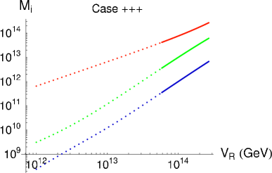
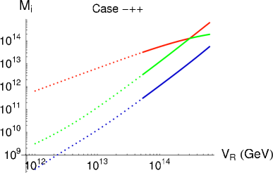
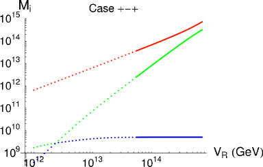
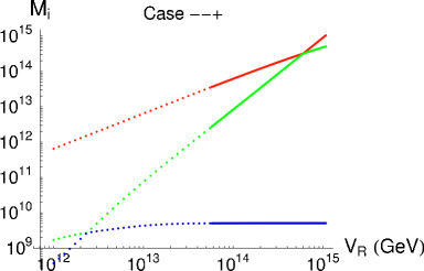
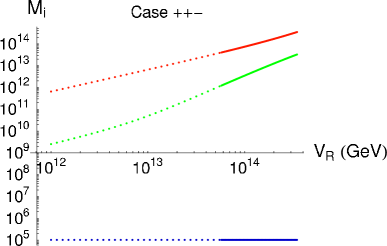
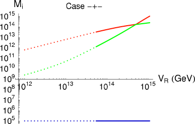
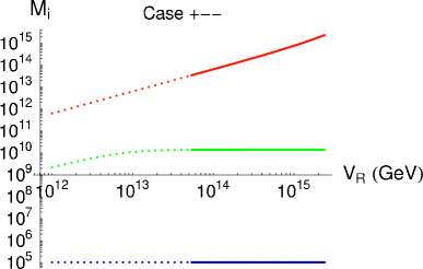
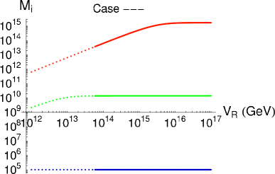
Figure 1: Right-handed neutrino masses as a function of $v_{R}$ for each of the 8 solutions $(+,+,+)$ to $(-,-,-)$ in the reference case of a hierarchical light neutrino mass spectrum with $m_{1}=10^{-3}$ eV, $\beta=\alpha$ and no CP violation beyond the CKM phase ($\delta=\Phi^{u}_{i}=\Phi^{d}_{i}=\Phi^{\nu}_{i}=\Phi^{e}_{i}=0$). The range of variation of $v_{R}$ is restricted by the requirement that $f_{3}\leq 1$. Dotted lines indicate a fine-tuning greater than $10\%$ in the $(3,3)$ entry of the light neutrino mass matrix.

Figs. 1 and 2 show the right-handed neutrino masses $M_{1,2,3}$ and their mixing angles $|(U_{f})_{12}|$, $|(U_{f})_{13}|$ and $|(U_{f})_{23}|$ as a function of $v_{R}$, for each of the 8 solutions $(+,+,+)$ to $(-,-,-)$, in the reference case $m_{1}=10^{-3}$ eV, $\beta=\alpha$ and $\delta=\Phi^{u}_{i}=\Phi^{d}_{i}=\Phi^{\nu}_{i}=\Phi^{e}_{i}=0$. Due to the interplay between the type I and type II contributions, the observed light neutrino masses and mixing angles are compatible with a large variety of right-handed neutrino mass spectra. As discussed in Subsection 2.2, one recovers the type I spectrum, characterized by the approximate hierarchy $M_{1}:M_{2}:M_{3}\sim m^{2}_{u}:m^{2}_{c}:m^{2}_{t}$, in the large $v_{R}$ region of solution $(-,-,-)$. Each eigenvalue $M_{i}$ reaches its type I value when the condition $4\alpha\beta\ll|z_{4-i}|^{2}$ is satisfied, i. e. when $v_{R}\gg 2v^{2}_{u}/|z_{4-i}|$. This explains why $M_{1}$ is constant over the considered range of values for $v_{R}$, while $M_{2}$ (resp. $M_{3}$) reaches a plateau only above $v_{R}\sim 10^{13}$ GeV (resp. $v_{R}\sim 5\times 10^{15}$ GeV). Symmetrically, the type II limit, characterized by the mild hierarchy $M_{1}:M_{2}:M_{3}\propto m_{1}:m_{2}:m_{3}$, corresponds to the large $v_{R}$ region of solution $(+,+,+)$. Finally, in the small $v_{R}$ region ($v_{R}\lesssim 10^{10}$ GeV) where there is a very strong cancellation between the type I and type II contributions, one finds an intermediate hierarchy $M_{1}:M_{2}:M_{3}\propto m_{u}:m_{c}:m_{t}$ (see Eq. (14) and discussion below). Although this region is not shown in the figures, one can already see that $M_{2}:M_{3}\sim m_{c}:m_{t}$ for $v_{R}=10^{12}$ GeV. These features of the right-handed neutrino mass spectra are expected to hold in other models where the Dirac mass matrix has a strong hierarchical structure, but is not necessarily related to the up quark mass matrix like in $SO(10)$ models.

The differences between the 8 different spectra plotted in Fig. 1 can be understood by noting that each $M_{i}$ can be associated (in the sense explained in Appendix B) with one of the eigenvalues of the matrix $X$, say $x_{j}$. If $x_{j}=x^{-}_{j}$ (“type I branch”), the corresponding right-handed neutrino mass $M_{i}$ first grows linearily with $v_{R}$, then reaches a plateau for $v_{R}\gg 2\sqrt{\alpha/\beta}\,v^{2}_{u}/|z_{j}|$, corresponding to $x_{j}\simeq-\beta/z_{j}$. If $x_{j}=x^{+}_{j}$ (“type II branch”), $M_{i}$ first grows linearly with $v_{R}$, then grows as $v^{2}_{R}$ for $v_{R}\gg 2\sqrt{\alpha/\beta}\,v^{2}_{u}/|z_{j}|$, corresponding to $x_{j}\simeq z_{j}/\alpha$. This allows one to classify the 8 different solutions as follows: the 4 solutions with $x_{3}=x^{-}_{3}$ are characterized by a constant value of the lightest right-handed neutrino mass, $M_{1}\simeq 10^{5}$ GeV (the “type I value” of $M_{1}$) over the considered range of values for $v_{R}$. Among these 4 solutions, the 2 solutions with $x_{2}=x^{-}_{2}$ also have a constant value of $M_{2}$ above $v_{R}\sim 10^{13}$ GeV. The 2 solutions with $x_{3}=x^{+}_{3}$ and $x_{2}=x^{-}_{2}$ are characterized by a constant value of $M_{1}$ above $v_{R}\sim 10^{13}$ GeV, $M_{1}=5\times 10^{9}$ GeV, and by a crossing of $M_{1}$ and $M_{2}$ close to $v_{R}=3\times 10^{12}$ GeV. Finally, the 2 solutions with $x_{3}=x^{+}_{3}$ and $x_{2}=x^{+}_{2}$ are characterized by a rising $M_{1}$.

As can be seen from Fig. 1, the perturbativity constraint forbids large values of $v_{R}$ in all solutions but $(-,-,-)$. The associated upper limit on $v_{R}$ ranges from $3\times 10^{14}$ to $3\times 10^{15}$ GeV (except for solution $(-,-,-)$ for which there is no such constraint on $v_{R}$), which excludes a breaking of $B-L$ above, at or just below the GUT scale. However, as discussed below, this conclusion strongly depends on the value of the ratio $\beta/\alpha$, assumed here to be $1$. If one requires in addition the absence of a strong cancellation between the type I and type II contributions to neutrino masses, the allowed values of $v_{R}$ are restricted to a rather small range.

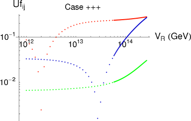
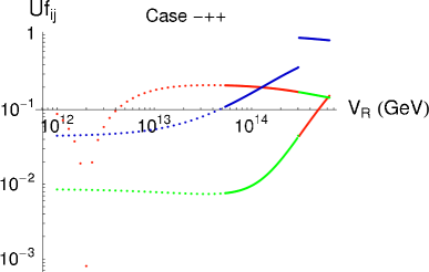
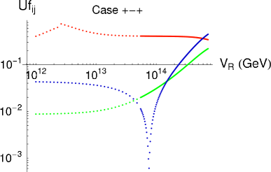
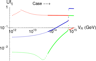
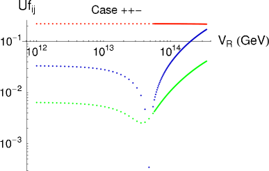
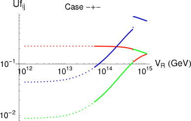
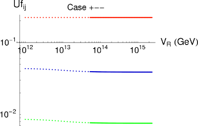
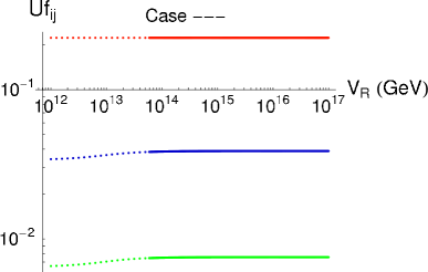
Figure 2: Right-handed neutrino mixing angles as a function of $v_{R}$ for each of the 8 solutions $(+,+,+)$ to $(-,-,-)$ in the reference case of a hierarchical light neutrino mass spectrum with $m_{1}=10^{-3}$ eV, $\beta=\alpha$ and no CP violation beyond the CKM phase ($\delta=\Phi^{u}_{i}=\Phi^{d}_{i}=\Phi^{\nu}_{i}=\Phi^{e}_{i}=0$). The red [dark grey] curve corresponds to $|(U_{f})_{12}|$, the green [light grey] curve to $|(U_{f})_{13}|$, and the blue [black] curve to $|(U_{f})_{23}|$.

Let us now consider the patterns of right-handed neutrino mixing angles (Fig. 2). As in the case of the mass eigenvalues, one can recognize known limits. The type I and the type II limits are recovered in the large $v_{R}$ region of solutions $(-,-,-)$ and $(+,+,+)$, respectively. The type I limit is characterized by small mixing angles, very close to the CKM angles, while in the type II limit where $f\rightarrow M_{\nu}/v_{L}$, the right-handed neutrino mixing angles are given by the PMNS angles (and since $\theta_{13}$ is close to its present experimental upper bound in the fit that we used, even $|(U_{f})_{13}|$ is relatively large in this limit). In the small $v_{R}$ region ($v_{R}\lesssim 10^{10}$ GeV), the mixing angles are close to the CKM angles in all solutions. This can be immediately understood in the $(+,+,+)$ and $(-,-,-)$ cases, in which, as discussed in Subsection 2.2, $f$ tends to $\pm\sqrt{\beta/\alpha}\,Y_{u}$ when $4\alpha\beta\gg|z_{3}|^{2}$; in the other cases, $U_{f}\approx U^{T}_{q}$ is a consequence of the hierarchical structure of the Dirac matrix (see Appendix B). Some striking features of the mixing patterns emerge. In solutions $(+,-,-)$ and $(-,-,-)$, the mixing angles are almost independent of $v_{R}$. In the other 6 solutions, the mixing angles evolve from $U_{f}\approx U^{T}_{q}$ at $v_{R}\lesssim 10^{10}$ GeV to significantly larger values at large $v_{R}$ (cancellations may occur for some specific values of $v_{R}$). The $(1,2)$ mixing angle is always of the order of the Cabibbo angle or greater, except in solutions $(+,+,+)$ and $(-,+,+)$ where a cancellation occurs close to $v_{R}=2\times 10^{12}$ GeV.

So far we only considered the reference case of a hierarchical light neutrino mass spectrum with $m_{1}=10^{-3}$ eV, $\beta=\alpha$ and no CP violation beyond the CKM case. It is interesting to see how different input parameters would affect the results of Figs. 1 and 2. In the following, we briefly discuss the impact on the right-handed neutrino mass spectrum of the ratio $\beta/\alpha$, of the high energy phases and of the type of the light neutrino mass hierarchy.

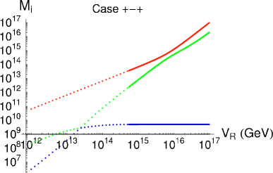
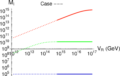
Figure 3: Effect of $\beta\neq\alpha$ on the right-handed neutrino masses. The input parameters are the same as in Fig. 1, except $\beta/\alpha=0.01$.

Let us first consider the effect of $\beta\neq\alpha$. As can be seen by comparing Figs. 1 and 3, taking $\beta\neq\alpha$ does not change the general shape of the solutions, but amounts to shift the curves $M_{i}=M_{i}(v_{R})$ along the horizontal axis according to $v_{R}\rightarrow\sqrt{\alpha/\beta}\,v_{R}$ (an analogous statement can be made about the curves $(U_{f})_{ij}=(U_{f})_{ij}(v_{R})$). For instance, in solution $(-,-,-)$, the type I limit is reached at larger $v_{R}$ values for $\beta/\alpha=0.01$ than for $\beta=\alpha$ (see the right panel of Fig. 3). Nevertheless the values of the $M_{i}$ corresponding to a plateau do not depend on $\beta/\alpha$. In particular, in the four solutions characterized by $x_{3}=x^{-}_{3}$, one has $M_{1}\simeq 10^{5}$ GeV over the considered range of values for $v_{R}$, irrespective of the value of $\beta/\alpha$. Finally, the value of $\beta/\alpha$ has a strong impact on the allowed range of values for $v_{R}$: as can be seen in the left panel of Fig. 3, the perturbativity constraint is more easily satisfied for large values of $v_{R}$ when $\beta/\alpha\ll 1$. This is due to the fact that the asymptotic value of $|f_{33}|$ in the small $v_{R}$ region, $\sqrt{\beta/\alpha}\,|(Y_{\nu})_{33}|$, is proportional to $\sqrt{\beta/\alpha}$. Conversely, the case $\beta/\alpha\gg 1$ is excluded because the perturbativity constraint $|f_{33}|<1$ is never satisfied, except in the type I limit of solution $(-,-,-)$. Therefore, perturbativity constrains the $SU(2)_{L}$ triplet mass to lie below the $B-L$ brealing scale (which might require a fine-tuning in the $SU(2)_{L}$ triplet mass matrix for $v_{R}\ll M_{GUT}$), except in the type I limit.

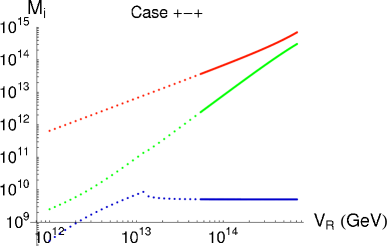
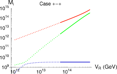
Figure 4: Effect of high-energy phases on the right-handed neutrino masses. The input parameters are the same as in Fig. 1, except $\Phi^{u}_{2}=\pi/4$ (left panel), $\Phi^{d}_{1}=\pi/4$ (right panel).

The effect of input CP-violating phases other than the CKM phase on the right-handed neutrino masses is illustrated in Fig. 4. In general, the presence of these phases only slightly affects the shape of the solutions, except in regions where a crossing of two mass eigenvalues occurs. Indeed, phases can lift isolated degeneracies between two eigenvalues (the curves repel one another instead of crossing), thus sensibly modifying the shape of the solution. An example of this effect is shown in Fig. 4, where the solution $(+,-,+)$ is displayed for two different choices of a non-zero high-energy phase, $\Phi^{u}_{2}=\pi/4$ (left panel) and $\Phi^{d}_{1}=\pi/4$ (right panel). These plots are to be compared with the corresponding plot in Fig. 1, where a crossing between $M_{1}$ and $M_{2}$ occurs at $v_{R}\simeq 3\times 10^{12}$ GeV. As for the right-handed neutrino mixing angles $(U_{f})_{ij}$, they are even more sensitive to input CP-violating phases than the $M_{i}$.

Finally, the right-handed neutrino mass and mixing patterns also depend on the light neutrino parameters that serve as an input in the reconstruction procedure, some of which are still unknown ($m_{1}$, $\mbox{sign}\,(\Delta m^{2}_{32})$, $\theta_{13}$, $\delta$ and the two Majorana phases contained in $P_{\nu}$). It has already been shown in the type I case that particular values of these parameters can drastically modify the pattern of right-handed neutrino masses obtained in the generic case [8]. It would be very interesting to investigate such effects in the case considered here; however, a general study of the dependence of the 8 right-handed neutrino spectra on the light neutrino mass parameters is beyond the scope of this paper. We just show in passing (Fig. 5) the impact of the type of the light neutrino mass hierarchy on right-handed neutrino masses, for the two solutions where the effect is the most significant.

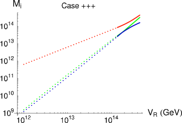
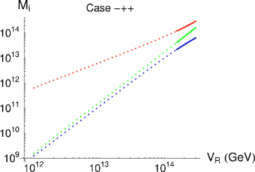
Figure 5: Effect of the light neutrino mass hierarchy on the right-handed neutrino masses. The input parameters are the same as in Fig. 1, except that the light neutrino mass hierarchy is inverted, with $m_{3}=10^{-3}$ eV and opposite CP parities for $m_{1}$ and $m_{2}$.

4 Leptogenesis

In the previous section, we showed on a particular $SO(10)$ example that the spectrum of possibilities to account for the experimental neutrino data in the presence of both type I and type II seesaw mechanisms is very rich. This has of course important implications for phenomena in which the presence of right-handed neutrinos and/or of a heavy $SU(2)_{L}$ triplet plays a role, such as leptogenesis and, in supersymmetric theories, lepton flavour violation.

In this section, we show that taking into account both seesaw contributions to neutrino masses opens up new possibilities for successful leptogenesis in $SO(10)$ GUTs. Since the model we consider is not fully realistic as it leads to wrong mass relations between charged fermions, we do not undertake a full study of leptogenesis including washout effects, but consider solely the value of the CP asymmetry. We do not try either to maximize the asymmetry by playing with all input parameters (in particular, we stick to a hierarchical light neutrino spectrum with $m_{1}=10^{-3}$ eV and the best fit values (21) and (22) for the oscillation parameters), but we restrict our attention to the impact of the input CP-violating phases.

In the scenario we are considering, it is natural to assume that the lightest right-handed neutrino is lighter than the $SU(2)_{L}$ triplet. Indeed, while the perturbativity constraint discussed in Subsection 3.2 requires $M_{\Delta_{L}}\lesssim v_{R}$, $M_{1}$ lies several orders of magnitude below $v_{R}$. Thus, one can safely assume that $M_{1}\ll M_{\Delta_{L}}$, in which case the lepton asymmetry is dominantly generated in out-of-equilibrium decays of the lightest right-handed (s)neutrino. The CP asymmetry $\epsilon_{N_{1}}\equiv\left[\Gamma(N_{1}\rightarrow lH)-\Gamma(N_{1}\rightarrow\bar{l}H^{\star})\right]/\left[\Gamma(N_{1}\rightarrow lH)+\Gamma(N_{1}\rightarrow\bar{l}H^{\star})\right]$ receives two contributions: the standard type I contribution $\epsilon^{I}_{N_{1}}$ [2, 25], and a contribution from a vertex diagram containing a virtual triplet, $\epsilon^{II}_{N_{1}}$ [26, 27]. In the case $M_{1}\ll M_{2,3}$ which is relevant here, they can be written as [27, 28]:

$$\epsilon^{I(II)}_{N_{1}}\ =\ \frac{3}{8\pi}\ \frac{\sum_{k,l}\mbox{Im}\left[Y_{1k}Y_{1l}\,(M^{I(II)}_{\nu})^{\star}_{kl}\right]}{(YY^{\dagger})_{11}}\ \frac{M_{1}}{v^{2}}\ ,$$ (24)

where $M^{I}_{\nu}\equiv-\beta\,Yf^{-1}Y$ and $M^{II}_{\nu}\equiv\alpha f$ are the type I and type II contributions to the neutrino mass matrix, respectively. The total CP asymmetry in $N_{1}$ decays then reads:

$$\epsilon_{N_{1}}\ =\ \epsilon^{I}_{N_{1}}+\epsilon^{II}_{N_{1}}\ =\ \frac{3}{8\pi}\ \frac{\sum_{k,l}\mbox{Im}\left[Y_{1k}Y_{1l}\,(M_{\nu})^{\star}_{kl}\right]}{(YY^{\dagger})_{11}}\ \frac{M_{1}}{v^{2}}\ .$$ (25)

In Eqs. (24) and (25), the Dirac couplings are expressed in the basis of charged lepton and right-handed neutrino mass eigenstates, i.e. $Y_{1k}\equiv(U^{\dagger}_{f}Y_{\nu})_{1k}$. Besides its obvious dependence on the light neutrino mass matrix and on the phases it contains, the CP asymmetry depends on the considered solution for the matrix $f$ and on the input parameters (in particular on the phases) through their influence on the values of $M_{1}$ and of the right-handed neutrino mixing angles $(U_{f})_{i1}$ ($i=1,2,3$).

The final baryon asymmetry is given by:

$$\frac{n_{B}}{s}\ =\ -1.48\times 10^{-3}\,\eta\,\epsilon_{N_{1}}\ ,$$ (26)

where $\eta$ is an efficiency factor that takes into account the initial population of right-handed (s)neutrinos, the out-of-equilibrium condition for their decays, and the subsequent dilution of the generated lepton asymmetry by wash-out processes [7]. For leptogenesis to be successful, Eq. (26) should reproduce the observed baryon-to-entropy ratio $n_{B}/s=(8.7\pm 0.3)\times 10^{-11}$ [29]. Detailed studies of thermal leptogenesis in the type I case (see e.g. Refs. [6, 7]) have shown that $\eta\geq 0.1$ over a significant portion of the parameter space; therefore thermal leptogenesis can succesfully generate the observed cosmological baryon asymmetry for $|\epsilon_{N_{1}}|\sim 10^{-6}$ (or even for $|\epsilon_{N_{1}}|\sim\mbox{few}\times 10^{-7}$ in the case of a thermal initial population of $N_{1}$ / $\tilde{N}_{1}$). Large efficiency factors can also be obtained in the presence of both type I and type II seesaw mechanisms [27].

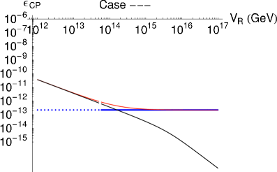
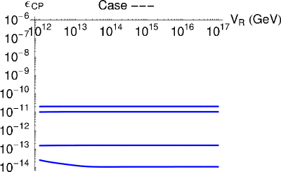
Figure 6: CP asymmetry $\epsilon_{1}$ as a function of $v_{R}$ for the solution $(-,-,-)$ in the case of a hierarchical light neutrino mass spectrum with $m_{1}=10^{-3}$ eV, $\beta=\alpha$, and no CP violation beyond the CKM phase (left panel) or different choices of CP-violating phases (right panel). On the left panel, the thin lines correspond to the contribution of right-handed neutrinos (red [grey] curve) and of the heavy triplet (black curve).

Figs. 6 to 8 show the absolute value of the CP asymmetry in $N_{1}$ decays as a function of $v_{R}$, for three representative solutions $(-,-,-)$, $(+,+,+)$ and $(+,-,+)$. Before commenting on these results, let us note that an upper bound on $\epsilon_{N_{1}}$ can be derived from Eq. (25) [27, 28]:

$$|\epsilon_{N_{1}}|\ \leq\ \epsilon^{max}_{N_{1}}\equiv\frac{3}{8\pi}\ \frac{M_{1}m_{max}}{v^{2}}\ \simeq\ 2\times 10^{-7}\left(\frac{M_{1}}{10^{9}\,\mbox{GeV}}\right)\left(\frac{m_{max}}{0.05\,\mbox{eV}}\right),$$ (27)

where $m_{max}\equiv\max\,(m_{1},m_{2},m_{3})$. From this one can already conclude that, for a generic hierarchical light neutrino mass spectrum, the four solutions characterized by $x_{3}=x^{-}_{3}$, which give $M_{1}\sim 10^{5}$ GeV for all values of $v_{R}$, fail to generate the observed baryon asymmetry from $N_{1}$ decays (we comment at the end of this section on possible flavour effects). This is confirmed by Fig. 6, which shows that, depending on the values of the CP-violating phases, $|\epsilon_{N_{1}}|$ ranges from $10^{-14}$ to $2\times 10^{-11}$ in the $(-,-,-)$ solution. As expected, the CP asymmetry is dominated by the type I contribution for large values of $v_{R}$, while the type I and the type II contributions become comparable and start cancelling each other below $v_{R}\sim 10^{14}$ GeV. The most noticeable fact here is that $\epsilon_{N_{1}}$ (like $M_{1}$) stays constant at its type I value even far away from the type I limit.

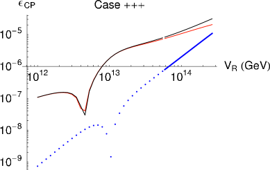
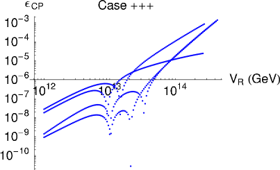
Figure 7: Same as Fig. 6 but for the solution $(+,+,+)$.

The four solutions characterized by $x_{3}=x^{+}_{3}$, which for $v_{R}>10^{13}$ GeV give either $M_{1}\sim 5\times 10^{9}$ GeV (case $x_{2}=x^{-}_{2}$) or $M_{1}>10^{10}$ GeV (case $x_{2}=x^{+}_{2}$), look much more promising. Indeed, solutions $(+,+,+)$ and $(-,+,+)$ (case $x_{2}=x^{+}_{2}$) yield large values of $\epsilon_{N_{1}}$, even in the absence of other sources of CP violation than the CKM phase (see Fig. 7). However, the effective mass parameter $\tilde{m}_{1}\equiv(YY^{\dagger})_{11}v^{2}/M_{1}$, which controls the out-of-equilibrium condition and the wash-out due to inverse $N_{1}$ decays, tends to be rather large (typically $\tilde{m}_{1}\sim 10^{-2}$ eV). The corresponding suppression of the final baryon asymmetry can be compensated for by larger values of $\epsilon_{N_{1}}$, but at the price of a heavier right-handed neutrino: one typically has $|\epsilon_{N_{1}}|>10^{-5}$ for $M_{1}\gtrsim 10^{11}$ GeV. Such values of $M_{1}$ are in conflict with the upper limit on the reheating temperature from gravitino overproduction, which depending on the gravitino mass and decay modes may lie between $10^{6}$ and $10^{10}$ GeV [30]. One may circumvent this problem by invoking a non-thermal mechanism for producing right-handed (s)neutrinos after inflation, e. g. decays of the inflaton field [31].

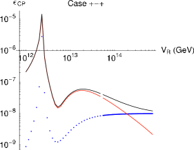
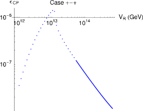
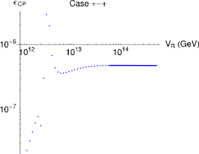
Figure 8: Same as Fig. 6 but for the solution $(+,-,+)$, with no CP violation beyond the CKM phase (left panel), $\Phi^{u}_{2}=\pi/4$ (middle panel) and $\Phi^{\nu}_{2}=\pi/4$ (right panel).

Solutions $(+,-,+)$ and $(-,-,+)$ (case $x_{2}=x^{-}_{2}$) are in principle better candidates for a successful thermal leptogenesis since they predict $M_{1}\sim 5\times 10^{9}$ GeV, a value that can lead to a sufficient CP asymmetry while being marginally compatible with the gravitino constraint. As shown by Fig. 8, the CP asymmetry generally reaches a plateau above $v_{R}\sim 10^{13}$ GeV, where depending on the phases it can be as large as $5\times 10^{-7}$ (interestingly enough, this may solely be due to low-energy CP-violating phases – see the right panel of Fig. 8). Such values of $\epsilon_{N_{1}}$ could be sufficient for generating the observed baryon asymmetry, provided that the wash-out processes are slow enough. However, the effective mass parameter $\tilde{m}_{1}$ tends to be too large, typically $\tilde{m}_{1}>10^{-2}$ eV. Larger values of $\epsilon_{N_{1}}$ can be obtained in the region where a strong cancellation between the type I and type II contributions to neutrino masses occur. In the left and right panels of Fig. 8, the peak located at $v_{R}\approx 3\times 10^{12}$ GeV is due to a near degeneracy between $M_{1}$ and $M_{2}$; there resonant leptogenesis [32] becomes possible. In the middle panel, the enhancement of $\epsilon_{N_{1}}$ around $v_{R}=10^{13}$ GeV is not related to any mass degeneracy and is simply an effect of the phase $\Phi^{u}_{2}$. In this case too, the wash-out of the generated lepton asymmetry is strong ($\tilde{m}_{1}\approx 0.03$ eV).

Before closing this section, let us comment on possible flavour effects [33, 34, 35, 36, 37], specializing for definiteness to the type I limit of solution $(-,-,-)$. The relevant quantities are the CP asymmetries in the decays of one right-handed neutrino flavour $N_{i}$ into one charged lepton flavour $l_{\alpha}$, defined as $\epsilon^{\alpha}_{i}\equiv\left[\Gamma(N_{i}\rightarrow l_{\alpha}H)-\Gamma(N_{i}\rightarrow\bar{l}_{\alpha}H^{\star})\right]/$ $\left[\Gamma(N_{i}\rightarrow lH)+\Gamma(N_{i}\rightarrow\bar{l}H^{\star})\right]$, as well as the parameters $\tilde{m}^{\alpha}_{i}\equiv|Y_{i\alpha}|^{2}v^{2}/M_{i}$, which control the out-of-equilibrium conditions and the main wash-out processes. Because of the smallness of its mass, including flavour effects in the decays of the lightest right-handed neutrino $N_{1}$ [36, 37] does not improve the situation; but it has been suggested that decays of the next-to-lightest right-handed neutrino $N_{2}$ (whose mass is $M_{2}\simeq 2\times 10^{10}$ GeV here) might lead to successful leptogenesis, without [38] or with [35] flavour effects. One interesting possibility [35] is that $N_{2}$ decays generate a large asymmetry in a specific lepton flavour that is only mildly erased by $N_{1}$ decays and inverse decays. Whether this can happen or not depends on the values of the parameters $\epsilon^{\alpha}_{2}$, $\tilde{m}^{\alpha}_{2}$ and $\tilde{m}^{\alpha}_{1}$ which we give in Table 1, together with the other flavoured parameters for completeness. In the case considered (hierarchical light neutrino mass spectrum with $m_{1}=10^{-3}$ eV, $\Phi^{\nu}_{2}=\pi/4$ and all other CP-violating phases but the CKM phase set to zero), we find that the lepton asymmetry is essentially generated in the tau flavour; unfortunately it is small ($\epsilon^{\tau}_{2}=1.4\times 10^{-7}$) and the wash-out by $N_{1}$ decays turns out to be strong ($\tilde{m}^{\tau}_{1}=2.2\times 10^{-2}$). Different choices of the CP-violating phases might however improve the situation.

parameter / lepton flavour	$\alpha=e$	$\alpha=\mu$	$\alpha=\tau$
$\epsilon^{\alpha}_{1}$	$2.7\times 10^{-13}$	$-6.0\times 10^{-12}$	$-1.5\times 10^{-11}$
$\epsilon^{\alpha}_{2}$	$5.6\times 10^{-11}$	$-1.5\times 10^{-9}$	$1.4\times 10^{-7}$
$\epsilon^{\alpha}_{3}$	$-1.8\times 10^{-14}$	$5.0\times 10^{-13}$	$-4.5\times 10^{-11}$
$\tilde{m}^{\alpha}_{1}$	$3.3\times 10^{-3}$ eV	$1.6\times 10^{-2}$ eV	$2.2\times 10^{-2}$ eV
$\tilde{m}^{\alpha}_{2}$	$5.9\times 10^{-4}$ eV	$1.1\times 10^{-2}$ eV	$3.5\times 10^{-2}$ eV
$\tilde{m}^{\alpha}_{3}$	$4.0\times 10^{-7}$ eV	$1.1\times 10^{-5}$ eV	$9.4\times 10^{-3}$ eV

Table 1: Parameters that control flavour effects in leptogenesis in the type I case (large $v_{R}$ limit of solution $(-,-,-)$), in the case of a hierarchical light neutrino mass spectrum with $m_{1}=10^{-3}$ eV, $\Phi^{\nu}_{2}=\pi/4$ and all other CP-violating phases but the CKM phase set to zero.

The above discussion shows that taking into account both the type I and the type II seesaw contributions to neutrino masses opens up new possibilities for successful leptogenesis in $SO(10)$ GUTs, even though, for the specific choice of input parameters made in this paper, the wash-out processes tend to be too strong. Different choices for the light neutrino mass parameters, or different combinations of the high-energy phases, could resolve this problem. Let us also recall that the results presented in this section were obtained using the mass relations (17), which need to be corrected. The inclusion of corrections leading to realistic charged fermion mass matrices, e.g. from the $\bf\overline{126}$ Higgs representation, is not expected to alter the gross qualitative features of the right-handed neutrino mass spectrum, but might modify the numerical values of $M_{1}$ and of the right-handed neutrino mixing angles, hence the predictions for leptogenesis.

5 Lepton flavour violation

In supersymmetric extensions of the Standard Model, lepton flavour violating (LFV) processes such as the charged lepton radiative decays $l_{j}\rightarrow l_{i}\gamma$ arise from loop diagrams involving sleptons and charginos/neutralinos. The relevant flavour-violating parameters are the off-diagonal entries of the slepton soft supersymmetry breaking mass matrices $(m^{2}_{\tilde{L}})_{ij}$, $(m^{2}_{\tilde{e}_{R}})_{ij}$ and $(m^{e\,2}_{RL})_{ij}\equiv A^{e}_{ij}v_{d}$, expressed in the flavour basis defined by the charged lepton mass eigenstates.

If the supersymmetry breaking mechanism is flavour blind, flavour violation in the slepton sector arises from radiative corrections induced by the flavour-violating couplings of heavy states populating the theory between the Planck scale and the electroweak scale. Here we must deal with two kinds of such couplings: the couplings of the right-handed neutrinos [3, 40, 41], $Y_{ki}$ (where $Y\equiv U^{\dagger}_{f}Y_{\nu}$), and the couplings of the heavy $SU(2)_{L}$ triplet [39], $f_{ij}$. Integrating the one-loop renormalization group equations in the lowest approximation, one obtains the following expressions for the flavour-violating (off-diagonal) entries of the soft supersymmetry breaking slepton mass matrices:

$$(m^{2}_{\tilde{L}})_{ij}\ \simeq\ -\,\frac{3m^{2}_{0}+A^{2}_{0}}{8\pi^{2}}\ C_{ij}\ ,\qquad(m^{2}_{\tilde{e}_{R}})_{ij}\ \simeq\ 0\ ,\qquad A^{e}_{ij}\ \simeq\ -\,\frac{3}{8\pi^{2}}\,A_{0}y_{e_{i}}C_{ij}\ ,$$ (28)

where the coefficients $C_{ij}$ encapsulate the dependence on the seesaw parameters:

$$C_{ij}\ \equiv\ \sum_{k}Y^{\star}_{ki}Y_{kj}\,\ln\!\left(\frac{M_{U}}{M_{k}}\right)+3\,(ff^{\dagger})_{ij}\,\ln\!\left(\frac{M_{U}}{M_{\Delta_{L}}}\right)\ .$$ (29)

Here $M_{U}$ is the scale at which universality among soft supersymmetry breaking parameters (at least in the slepton and Higgs sector) is assumed. In the following, we take $M_{U}=10^{17}$ GeV, close to the Landau pole $\Lambda_{10}$ where the theory becomes non perturbative. Neglecting the smaller contribution of the flavour-violating $A$-term and working in the mass insertion approximation, one can schematically write the branching ratio for $l_{j}\rightarrow l_{i}\gamma$ as:

$$\frac{\mbox{BR}\,(l_{j}\rightarrow l_{i}\gamma)}{\mbox{BR}\,(l_{j}\rightarrow l_{i}\bar{\nu}_{i}\nu_{j})}\ \propto\ \frac{|(m^{2}_{\tilde{L}})_{ij}|^{2}}{\bar{m}^{8}_{\tilde{L}}}\ \tan^{2}\beta\ F_{Susy}\ ,$$ (30)

where $\bar{m}^{2}_{\tilde{L}}$ is the average slepton doublet mass, and $F_{Susy}$ is a function of the supersymmetric mass parameters and of $\tan\beta$. The experimental upper limits $\mbox{BR}\,(\mu\rightarrow e\gamma)<1.2\times 10^{-11}$ [42] and $\mbox{BR}\,(\tau\rightarrow\mu\gamma)<6.8\times 10^{-8}$ [43] can then be translated into upper bounds on the $C_{12}$ and $C_{23}$ coefficients as a function of the superpartner masses and of $\tan\beta$ [44]. If we require that the mSUGRA parameters $m_{0}$ and $M_{1/2}$ do not exceed $\sim 1$ TeV, then from Fig. 3 of Ref. [45] we can read the approximate upper bounds $|C_{12}|\lesssim 0.1$ and $|C_{23}|\lesssim 10$ for a benchmark value of $\tan\beta=10$. For different values of $\tan\beta$, the upper bounds approximately scale as $10/\tan\beta$.

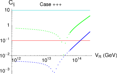
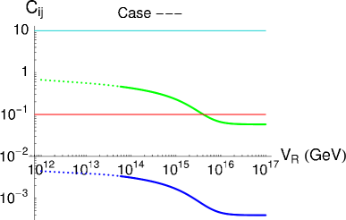
Figure 9: Coefficients $C_{12}$ and $C_{23}$ as a function of $v_{R}$ for the solutions $(+,+,+)$ and $(-,-,-)$ in the case of a hierarchical light neutrino mass spectrum with $m_{1}=10^{-3}$ eV, $\beta=\alpha$, and no CP violation beyond the CKM phase. The green [light grey] curve corresponds to $|C_{23}|$, and the blue [black] curve to $|C_{12}|$. The horizontal lines indicate the “experimental” constraints $|C_{23}|<10$ and $|C_{12}|<0.1$ (see text).

In Fig. 9, we compare the values of the coefficients $|C_{12}|$ and $|C_{23}|$ in solutions $(+,+,+)$ and $(-,-,-)$ with the “experimental constraints” $|C_{12}|<0.1$ and $|C_{23}|<10$, assuming $\beta=\alpha$ and $M_{\Delta_{L}}=v_{R}$. The plot in the left panel of Fig. 9 is representative of all solutions but $(+,-,-)$ and $(-,-,-)$. One finds that $\mbox{BR}\,(\tau\rightarrow\mu\gamma)$ lies below the experimental constraint for all allowed values of $v_{R}$ (unless $\tan\beta$ is large and/or some superpartners are light), but it could be accessible to future experiments for $v_{R}\gtrsim 10^{14}$ GeV. The decay $\mu\rightarrow e\gamma$ is much closer to its present experimental upper limit for larger values of $v_{R}$, and even exceeds it for $v_{R}>10^{14}$ GeV (with the assumed values of the supersymmetric parameters). Solutions $(-,-,-)$ and $(+,-,-)$ have a completely different behaviour; for these solutions both $\mbox{BR}\,(\tau\rightarrow\mu\gamma)$ and $\mbox{BR}\,(\mu\rightarrow e\gamma)$ are well below their experimental uper limits for all values of $v_{R}$.

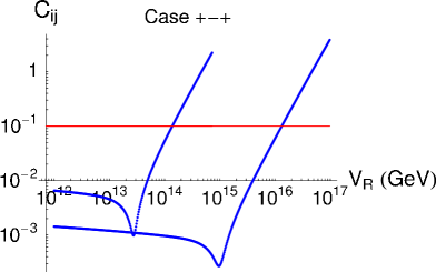
Figure 10: Effect of $\beta\neq\alpha$ on $C_{12}$ for the solution $(+,-,+)$. The input parameters are the same as in Fig. 9, except that $\beta/\alpha=1$ and $M_{\Delta_{L}}=v_{R}$ for the left curve, while $\beta/\alpha=0.01$ and $M_{\Delta_{L}}=0.1v_{R}$ for the right curve.

We have checked numerically that, except for the large $v_{R}$ regions of solutions $(-,-,-)$ and $(+,-,-)$, the type II contribution always dominates in $C_{12}$ and $C_{23}$ (at least for $\beta\sim\alpha$). This can easily be understood by noting that, due to the relation $Y_{\nu}=Y_{u}$, the type I contribution is suppressed by the small CKM angles. The coefficients $C_{ij}$ thus essentially reflect the structure of the matrix $f$, and like the matrix $f$, they have a strong sensitivity to the CP-violating phases and to the ratio $\beta/\alpha$. The impact of $\beta/\alpha$ is shown in Fig. 10. One can see that, for a fixed value of $v_{R}$, a lower ratio $\beta/\alpha$ results in reduced LFV rates.

To summarize, in the considered class of $SO(10)$ models, LFV processes are dominated by the type II contribution in most of the parameter space of the 8 solutions. The predictions lie significantly below the experimental upper limits, except for the large $v_{R}$ region of most solutions, where depending on the values of the supersymmetric parameters $\mu\rightarrow e\gamma$ can even exceed its present upper limit. The expected improvement of the experimental sensitivity to LFV processes will strongly constrain this region.

6 Conclusions

The procedure presented in this paper for reconstructing the matrix $f$ of the left-right symmetric seesaw mechanism from the light neutrino mass parameters can be applied in any theory with an underlying left-right symmetry which predicts (or at least constrains) the Dirac mass matrix. The 8 solutions for the $f_{ij}$ couplings can then be used to study a number of issues in which the presence of right-handed neutrinos or heavy $SU(2)_{L(R)}$ triplets (or other heavy states embedded in the same GUT representation) plays a role, such as leptogenesis, lepton flavour violation, electric dipole moments of charged leptons, or proton decay [46]. Some of these processes (e.g. $\mu\rightarrow e\gamma$) put strong constraints on the 8 solutions, and might even exclude some of them. The reconstruction procedure can also be used as a tool to investigate the flavour structure of the right-handed neutrino mass matrix and to make progress in the quest for a flavour theory.

In this paper, we applied the procedure to a particular class of supersymmetric $SO(10)$ models with two $\bf 10$-dimensional and a pair of $\bf 126\oplus\overline{126}$ representations in the Higgs sector. We found a large variety of right-handed neutrino spectra compatible with the observed neutrino data, opening new possibilities for successful leptogenesis in $SO(10)$ GUTs. We also studied LFV processes in these models and found large triplet contributions in most solutions, especially in the region of large $v_{R}$ values. As a byproduct of our study, we found interesting constraints on the breaking scale of the $B-L$ symmetry, hence on the masses of the heavy states which play a role in issues such as gauge coupling unification. In particular, for $\beta\sim\alpha$, the perturbativity constraint excludes values of $v_{R}$ above a few $(10^{14}-10^{15})$ GeV, depending on the solution (except for the $(-,-,-)$ solution). LFV processes further restrict the range of allowed values for $v_{R}$ as a function of the supersymmetric parameters. Also, it is interesting to note that the region of values for $v_{R}$ that is disfavoured by fine-tuning arguments is the one in which gauge coupling unification is problematic.

As mentioned earlier, cancellations between the type I and type II contributions to neutrino masses, rather than being accidental, could be due to some (broken) symmetry ensuring a proportionality relation between the right-handed neutrino and triplet couplings, $f\propto Y_{\nu}$. This would be particularly relevant for some interesting possibilities for leptogenesis that occur in the fine-tuned region, or close to it. Interestingly enough, such a proportionality relation automatically follows from the embedding of the $SO(10)$ model in an $E_{6}$ GUT with a $\bf 27_{H}\oplus\overline{27}_{H}$ and a $\bf 351^{\prime}\oplus\overline{351}^{\prime}$ pairs in the Higgs sector, in such a way that the $\bf 351^{\prime}$ representation contains the $\bf\overline{126}$, $\bf 54$ and $\bf 10_{2}$ representations of $SO(10)$, while $\bf 27_{H}$ contains $\bf 10_{1}$. With this embedding, both couplings $\bf 16_{i}16_{j}10_{2}$ and $\bf 16_{i}16_{j}\overline{126}$ come from the $\bf 27_{i}27_{j}351^{\prime}$ superpotential term. Assuming that the doublet that couples to up quarks in $\bf 10_{1}$ does not acquire a vev, one obtains $f\propto Y_{\nu}$. Therefore the presence of a fine-tuning in the seesaw mass formula, rather than being unnatural, could point to an extended unification in $E_{6}$.

A few simplifying assumptions were made in this paper. First, the gauge symmetry breaking aspects of the models (including the issues of doublet-triplet splitting and gauge coupling unification) were not taken into account; second, corrections to the “wrong” mass relation $M_{d}=M_{e}$ were neglected. There are good reasons to believe that these approximations are justified at the qualitative level. Indeed, the main features of the right-handed neutrino spectra are dictated by the strong hierarchical structure of the Dirac mass matrix, and would not be spoiled by small corrections to the basic $SO(10)$ mass relations. Nevertheless a more detailed analysis using realistic mass relations is needed in order to obtain quantitative predictions, in particular for leptogenesis. Also, a more systematic scan over the input parameters (most notably the high-energy phases and the light neutrino masses and mixings) would probably provide useful information. Work along these lines is in progress.

Acknowledgments

We aknowledge useful discussions with M. Frigerio and Th. Hambye. This work has been supported in part by the RTN European Program MRTN-CT-2004-503369 and by the French Program “Jeunes Chercheurs” of the Agence Nationale de la Recherche (ANR-05-JCJC-0023).

Appendix A Perturbativity constraint on the $f_{ij}$ couplings

In this appendix, we discuss the constraint coming from the requirement that the couplings $f_{ij}$ remain in the perturbative regime up to the scale at which the unified gauge coupling $g_{10}$ blows up, $\Lambda_{10}=M_{GUT}\exp[-\frac{8\pi^{2}}{b_{10}\,g^{2}_{10}(M_{GUT})}]$, where $b_{10}$ is the $SO(10)$ beta function coefficient (this Landau pole is due to the presence of a $\bf 126\oplus\overline{126}$ pair in the Higgs sector, which gives a large contribution to $b_{10}$).

Above $M_{GUT}$, the running of the $f_{ij}$ couplings is governed by the renormalization group equation:

$$\frac{df_{ij}}{dt}\ =\ \frac{1}{2}\,\mbox{Tr}(f^{\dagger}f)f_{ij}+15\,(ff^{\dagger}f)_{ij}-\frac{95}{2}\,g^{2}_{10}f_{ij}+\cdots\ ,$$ (31)

where the dots stand for the contribution of the other superpotential couplings, which we assume to play a subdominant role in the regime where the $f_{ij}$’s are large. Assuming a hierarchy between the eigenvalues, $f_{1,2}\ll f_{3}$, one finds a critical value $f^{\rm crit.}_{3}(M_{GUT})=\sqrt{(95-2b)/31}\,g_{10}(M_{GUT})$ above which $f_{3}$ diverges before the Landau pole $\Lambda_{10}$ is reached. As an example, if the Higgs sector contains a $\bf 45$ and a $\bf 54$ representations in addition to the two $\bf 10$’s and to the $\bf 126\oplus\overline{126}$ pair, one obtains $\Lambda_{10}=1.5\times 10^{17}$ GeV and $f^{\rm crit.}_{3}(M_{GUT})\simeq 2$, where we have used $\alpha_{10}(M_{GUT})=1/24$ and $M_{GUT}=2\times 10^{16}$ GeV. Since the running of the $f_{ij}$’s below $M_{GUT}$ is much milder due to the decoupling of the heavy states, we can safely take $f_{3}<1$ as a perturbativity constraint at the scale where the $f_{ij}$’s are determined.

In the above, we have implicitly assumed that $v_{R}\leq M_{GUT}$. If this is not the case, $SO(10)$ is broken into $SU(5)$ at the scale $v_{R}$, above $M_{GUT}$; as a result the running of the $f_{ij}$’s above $M_{GUT}$ is slower than in the case $v_{R}\leq M_{GUT}$, and the Landau pole $\Lambda_{10}$ is shifted towards a larger scale. In spite of these differences, $f_{3}<1$ remains a relevant perturbativity constraint.

Appendix B Some useful analytical formulae

In this appendix, we provide analytical approximations that can be useful to understand the results of the reconstruction procedure described in Subsection 2.1. Although we follow the assumptions of Section 3, with $Y_{\nu}=Y_{u}$ in the basis of charged lepton mass eigenstates, the formulae presented below are more generally valid in the case of a hierarchical Dirac matrix $Y_{\nu}$, with eigenvalues $y_{1}\ll y_{2}\ll y_{3}$ and small mixing angles.

Let us first perform the diagonalization of the matrix $Z$, assuming for definiteness that the light neutrino mass spectrum is hierarchical ($m_{1}<m_{2}\ll m_{3}$). Using the notations of Subsection 3.1 and choosing $Y^{1/2}=U^{T}_{q}\hat{Y}^{1/2}_{u}$, we have:

$$Z\ =\ \hat{Y}^{-1/2}_{u}N\hat{Y}^{-1/2}_{u}\ ,\qquad N\ \equiv\ (U^{\star}_{q}U^{\star}_{l}\hat{M}_{\nu}U^{\dagger}_{l}U^{\dagger}_{q})/m_{3}\ .$$ (32)

Since $m_{2}/m_{3}\approx 0.2$ and two of the three lepton mixing angles are large (with $s_{23}\approx 1/\sqrt{2}$, $s_{12}\approx 1/\sqrt{3}$ and $s_{13}\lesssim 0.2$), the matrix $N$ has a very moderate hierarchy. We can parametrize it as:

$$N\ =\ \left(\begin{array}[]{ccc}a&b&c\\ b&d&e\\ c&e&f\end{array}\right)\ ,$$ (33)

with $|a|,|b|,|c|\sim m_{2}/m_{3}$, $|d|,|e|,|f|\sim 1$ and $|df-e^{2}|\sim m_{2}/m_{3}$. It is convenient to define the quantities:

$$\Delta_{11}\ \equiv\ df-e^{2}\ , \Delta_{12}\ \equiv\ bf-ce\ , \Delta_{13}\ \equiv\ be-cd\ ,$$ (34)

$$\Delta_{22}\ \equiv\ af-c^{2}\ , \Delta_{23}\ \equiv\ ae-bc\ , \Delta_{33}\ \equiv\ ad-b^{2}\ .$$ (35)

All $\Delta_{ij}$ are of order $m_{2}/m_{3}$, and $|\det N|=|a\Delta_{11}-b\Delta_{12}+c\Delta_{13}|=m_{1}m_{2}/m^{2}_{3}<(m_{2}/m_{3})^{2}$. The hierarchical structure of the matrix $Z$ is essentially determined by the up quark Yukawa couplings:

$$Z\ =\ \left(\begin{array}[]{ccc}a/y_{u}&b/\sqrt{y_{u}y_{c}}&c/\sqrt{y_{u}y_{t}}\\ b/\sqrt{y_{u}y_{c}}&d/y_{c}&e/\sqrt{y_{c}y_{t}}\\ c/\sqrt{y_{u}y_{t}}&e/\sqrt{y_{c}y_{t}}&f/y_{t}\end{array}\right).$$ (36)

The roots of the polynomial equation $\det(Z-z\mathbf{1})=0$ are obviously all distinct, hence $Z$ can be diagonalized by a complex orthogonal matrix $O_{Z}$:

$$Z\ =\ O_{Z}\left(\begin{array}[]{ccc}z_{1}&0&0\\ 0&z_{2}&0\\ 0&0&z_{3}\end{array}\right)O^{T}_{Z}\ ,$$ (37)

$$z_{1}\ =\ \frac{\det N}{\Delta_{33}}\,y^{-1}_{t}\ ,\qquad z_{2}\ =\ \frac{\Delta_{33}}{a}\,y^{-1}_{c}\ ,\qquad z_{3}\ =\ a\,y^{-1}_{u}\ ,$$ (38)

$$O_{Z}\ =\ \left(\begin{array}[]{ccc}\frac{\Delta_{13}}{\Delta_{33}}\,\sqrt{y_{u}/y_{t}}&-\frac{b}{a}\,\sqrt{y_{u}/y_{c}}&1\\ -\frac{\Delta_{23}}{\Delta_{33}}\,\sqrt{y_{c}/y_{t}}&1&\frac{b}{a}\,\sqrt{y_{u}/y_{c}}\\ 1&\frac{\Delta_{23}}{\Delta_{33}}\,\sqrt{y_{c}/y_{t}}&\frac{c}{a}\,\sqrt{y_{u}/y_{t}}\end{array}\right)\ ,$$ (39)

where we have ordered the $z_{i}$ in such a way that $|z_{1}|<|z_{2}|<|z_{3}|$. In Eqs. (38) and (39), the neglected terms are of relative order $y_{u}/y_{c}$, $y_{c}/y_{t}$ with respect to the dominant terms.

We can now reconstruct the 8 solutions for the matrix $f$. For a given choice of ($x_{1}$, $x_{2}$, $x_{3}$), the matrix $f$ is given by $f=U^{T}_{q}\hat{Y}^{1/2}_{u}X\hat{Y}^{1/2}_{u}U_{q}$, with $X=O_{Z}\mbox{Diag}\,(x_{1},x_{2},x_{3})O^{T}_{Z}$. The eigenvalues $f_{i}$ are obtained by diagonalizing $f$ with a unitary matrix $U_{f}$, Eq. (8). Alternatively, one can diagonalize the matrix $\tilde{X}\equiv\hat{Y}^{1/2}_{u}X\hat{Y}^{1/2}_{u}$, which is related to $f$ by $f=U^{T}_{q}\tilde{X}U_{q}$, and has therefore the same eigenvalues:

$$\tilde{X}\ =\ U_{\tilde{X}}\hat{f}U^{T}_{\tilde{X}}\ ,\qquad U_{\tilde{X}}U^{\dagger}_{\tilde{X}}=\mathbf{1}\ ,$$ (40)

the unitary matrix that brings $f$ to its diagonal form being given by $U_{f}=U^{T}_{q}U_{\tilde{X}}$. It does not seem to be possible to derive simple analytical formulae for the $f_{i}$ that would hold for any value of $\alpha$ and $\beta$. However, one can easily obtain approximate formulae in the regions of ($\alpha$, $\beta$) values where the $x_{i}$ satisfy some hierarchy requirements, as we show below. Let us first define the following quantities:

$$\bar{x}_{1}\ \equiv\ y_{t}\,x_{1}\ ,\qquad\bar{x}_{2}\ \equiv\ y_{c}\,x_{2}\ ,\qquad\bar{x}_{3}\ \equiv\ y_{u}\,x_{3}\ .$$ (41)

The $f^{2}_{i}$ are given by the roots of the characteristic equation:

$$\det(\tilde{X}\tilde{X}^{\star}-f^{2}_{i}\mathbf{1})\ =\ -f^{6}_{i}+C_{1}f^{4}_{i}-C_{2}f^{2}_{i}+C_{3}\ =\ 0,$$ (42)

with (up to subdominant terms of order $y_{u}/y_{c}$, $y_{c}/y_{t}$ in the coefficients of the $\bar{x}_{i}$ monomials):

$$C_{1} = \left(\frac{|a|^{2}+|b|^{2}+|c|^{2}}{|a|^{2}}\right)^{\!2}\,|\bar{x}_{3}|^{2}+\left(\frac{|\Delta_{23}|^{2}+|\Delta_{33}|^{2}}{|\Delta_{33}|^{2}}\right)^{\!2}\,|\bar{x}_{2}|^{2}+|\bar{x}_{1}|^{2}$$

$$+\ \left\{\left(\frac{b^{\star}}{a^{\star}}+\frac{c^{\star}\Delta_{23}}{a^{\star}\Delta_{33}}\right)^{\!2}\bar{x}_{2}\bar{x}^{\star}_{3}+\left(\frac{\Delta^{\star}_{23}}{\Delta^{\star}_{33}}\right)^{\!2}\bar{x}_{1}\bar{x}^{\star}_{2}+\left(\frac{c^{\star}}{a^{\star}}\right)^{\!2}\bar{x}_{1}\bar{x}^{\star}_{3}+\mbox{c.c.}\right\}\,,$$

$$C_{2} = \left(\frac{|\Delta_{13}|^{2}+|\Delta_{23}|^{2}+|\Delta_{33}|^{2}}{|\Delta_{33}|^{2}}\right)^{\!2}\,|\bar{x}_{2}\bar{x}_{3}|^{2}+\left(\frac{|a|^{2}+|b|^{2}}{|a|^{2}}\right)^{\!2}\,|\bar{x}_{1}\bar{x}_{3}|^{2}+|\bar{x}_{1}\bar{x}_{2}|^{2}$$

$$+\ \left\{\left(\frac{\Delta^{\star}_{23}}{\Delta^{\star}_{33}}+\frac{b\Delta^{\star}_{13}}{a\Delta^{\star}_{33}}\right)^{\!2}\bar{x}_{1}\bar{x}^{\star}_{2}|\bar{x}_{3}|^{2}+\left(\frac{\Delta^{\star}_{13}}{\Delta^{\star}_{33}}\right)^{\!2}\bar{x}_{1}\bar{x}^{\star}_{3}|\bar{x}_{2}|^{2}+\left(\frac{b^{\star}}{a^{\star}}\right)^{\!2}\bar{x}_{2}\bar{x}^{\star}_{3}|\bar{x}_{1}|^{2}+\mbox{c.c.}\right\}\,,$$

$$C_{3} = |\bar{x}_{1}\bar{x}_{2}\bar{x}_{3}|^{2}\ .$$

Using the fact that $C_{1}=f^{2}_{1}+f^{2}_{2}+f^{2}_{3}$, $C_{2}=f^{2}_{1}f^{2}_{2}+f^{2}_{1}f^{2}_{3}+f^{2}_{2}f^{2}_{3}$ and $C_{3}=f^{2}_{1}f^{2}_{2}f^{2}_{3}$, one immediately sees that, when there is a significant hierarchy between the $\bar{x}_{i}$, the $f_{i}$ are given by the $\bar{x}_{i}$ times an order one coefficient. More precisely, one has:

$$f_{1}\simeq\sqrt{C_{3}/C_{2}}\ \sim\ \bar{x}_{min}\ ,\qquad f_{2}\simeq\sqrt{C_{2}/C_{1}}\ \sim\ \bar{x}_{middle}\ ,\qquad f_{3}\simeq\sqrt{C_{1}}\ \sim\ \bar{x}_{max}\ ,$$ (44)

where $\bar{x}_{max}\equiv\max(|\bar{x}_{1}|,|\bar{x}_{2}|,|\bar{x}_{3}|)$, $\bar{x}_{min}\equiv\min(|\bar{x}_{1}|,|\bar{x}_{2}|,|\bar{x}_{3}|)$ and $\bar{x}_{middle}$ is the remaining $\bar{x}_{i}$. In the case $|\bar{x}_{1}|\ll|\bar{x}_{2}|\ll|\bar{x}_{3}|$, this reads:

$$f_{1}\ \simeq\ \frac{|\Delta_{33}|^{2}}{|\Delta_{13}|^{2}+|\Delta_{23}|^{2}+|\Delta_{33}|^{2}}\ |\bar{x}_{1}|\ ,\qquad f_{2}\ \simeq\ \frac{|a|^{2}(|\Delta_{13}|^{2}+|\Delta_{23}|^{2}+|\Delta_{33}|^{2})}{(|a|^{2}+|b|^{2}+|c|^{2})|\Delta_{33}|^{2}}\ |\bar{x}_{2}|\ ,$$

$$f_{3}\ \simeq\ \frac{|a|^{2}+|b|^{2}+|c|^{2}}{|a|^{2}}\ |\bar{x}_{3}|\ ,$$ (45)

while in the case $|\bar{x}_{3}|\ll|\bar{x}_{2}|\ll|\bar{x}_{1}|$, one has:

$$f_{3}\ \simeq\ |\bar{x}_{1}|\ ,\qquad f_{2}\ \simeq\ |\bar{x}_{2}|\ ,\qquad f_{1}\ \simeq\ |\bar{x}_{3}|\ ,$$ (46)

etc. When the hierarchy between the $\bar{x}_{i}$ is not so pronounced, Eq. (44) is no longer a good approximation. In the case $\bar{x}_{min}\ll\bar{x}_{middle}\leq\bar{x}_{max}$, however, one still has:

$$f_{1}\ \simeq\ \sqrt{C_{3}/C_{2}}\ \sim\ \bar{x}_{min}\ ,$$ (47)

while in the case $\bar{x}_{min}\leq\bar{x}_{middle}\ll\bar{x}_{max}$:

$$f_{3}\ \simeq\ \sqrt{C_{1}}\ \sim\ \bar{x}_{max}\ .$$ (48)

The formulae for the mixing angles are more involved, but they simplify for some $\bar{x}_{i}$ hierarchies. It is convenient to write $\tilde{X}$ as:

$$\tilde{X}\ =\ \bar{x}_{3}\left(\begin{array}[]{ccc}1&\frac{b}{a}&\frac{c}{a}\\ \frac{b}{a}&\frac{b^{2}}{a^{2}}&\frac{bc}{a^{2}}\\ \frac{c}{a}&\frac{bc}{a^{2}}&\frac{c^{2}}{a^{2}}\end{array}\right)\ +\ \bar{x}_{2}\left(\begin{array}[]{ccc}\frac{b^{2}}{a^{2}}\,\frac{y^{2}_{u}}{y^{2}_{c}}&-\frac{b}{a}\,\frac{y_{u}}{y_{c}}&-\frac{b\Delta_{23}}{a\Delta_{33}}\,\frac{y_{u}}{y_{c}}\\ -\frac{b}{a}\,\frac{y_{u}}{y_{c}}&1&\frac{\Delta_{23}}{\Delta_{33}}\\ -\frac{b\Delta_{23}}{a\Delta_{33}}\,\frac{y_{u}}{y_{c}}&\frac{\Delta_{23}}{\Delta_{33}}&\frac{\Delta^{2}_{23}}{\Delta^{2}_{33}}\end{array}\right)$$ (55)

$$+\ \bar{x}_{1}\left(\begin{array}[]{ccc}\frac{\Delta^{2}_{13}}{\Delta^{2}_{33}}\,\frac{y^{2}_{u}}{y^{2}_{t}}&-\frac{\Delta_{13}\Delta_{23}}{\Delta^{2}_{33}}\,\frac{y_{u}y_{c}}{y^{2}_{t}}&\frac{\Delta_{13}}{\Delta_{33}}\,\frac{y_{u}}{y_{t}}\\ -\frac{\Delta_{13}\Delta_{23}}{\Delta^{2}_{33}}\,\frac{y_{u}y_{c}}{y^{2}_{t}}&\frac{\Delta^{2}_{23}}{\Delta^{2}_{33}}\,\frac{y^{2}_{c}}{y^{2}_{t}}&-\frac{\Delta_{23}}{\Delta_{33}}\,\frac{y_{c}}{y_{t}}\\ \frac{\Delta_{13}}{\Delta_{33}}\,\frac{y_{u}}{y_{t}}&-\frac{\Delta_{23}}{\Delta_{33}}\,\frac{y_{c}}{y_{t}}&1\end{array}\right)\ ,$$ (59)

where subdominant terms of relative order $y_{u}/y_{c}$ and $y_{c}/y_{t}$ are understood in each entry of the matrices multiplying $\bar{x}_{1}$, $\bar{x}_{2}$ and $\bar{x}_{3}$. Let us first consider the hierarchy $|\bar{x}_{1}|,|\bar{x}_{2}|\ll|\bar{x}_{3}|$. In this case, $\tilde{X}$ is dominated by the contribution proportional to $\bar{x}_{3}$ in Eq. (59), and $U_{\tilde{X}}$ is given by:

$$U_{\tilde{X}}\ \simeq\ \left(\begin{array}[]{ccc}\tilde{a}&0&\bar{a}\\ -\frac{\bar{a}^{\star}\bar{b}}{\tilde{a}}&\frac{\bar{c}^{\star}}{\tilde{a}}&\bar{b}\\ -\frac{\bar{a}^{\star}\bar{c}}{\tilde{a}}&-\frac{\bar{b}^{\star}}{\tilde{a}}&\bar{c}\end{array}\right)\left(\begin{array}[]{ccc}a^{\star}_{12}&b_{12}&0\\ -b^{\star}_{12}&a_{12}&0\\ 0&0&1\end{array}\right)P\ ,$$ (60)

where $(\bar{a},\bar{b},\bar{c})\equiv(a,b,c)/\sqrt{|a|^{2}+|b|^{2}+|c|^{2}}$, $\tilde{a}\equiv\sqrt{1-|\bar{a}|^{2}}$, $P$ is a diagonal matrix of phases, $|a_{12}|^{2}+|b_{12}|^{2}=1$, and $a_{12}$ and $b_{12}$ depend on the subdominant terms in $\tilde{X}$. After multiplication by $U^{T}_{q}$, this gives:

$$|(U_{f})_{12}| \simeq \left|\tilde{a}b_{12}+(\bar{c}^{\star}a_{12}-\bar{a}^{\star}\bar{b}b_{12})V_{cd}\,e^{i(\Phi^{u}_{2}-\Phi^{u}_{1})}/\tilde{a}\right|\ \gtrsim\ \lambda\ ,$$ (61)

$$|(U_{f})_{13}| \simeq \left|\bar{a}+\bar{b}\,V_{cd}\,e^{i(\Phi^{u}_{2}-\Phi^{u}_{1})}\right|\ \sim\ 1\ ,$$ (62)

$$|(U_{f})_{23}| \simeq \left|\bar{b}+\bar{a}\,V_{us}\,e^{-i(\Phi^{u}_{2}-\Phi^{u}_{1})}\right|\ \sim\ 1\ .$$ (63)

Thus, the hierarchy $|\bar{x}_{1}|,|\bar{x}_{2}|\ll|\bar{x}_{3}|$ leads to large right-handed neutrino mixing angles (cancellations are possible in Eqs. (61)-(63) though).

Let us then consider the hierarchy $|\bar{x}_{1}|,|\bar{x}_{3}|\ll|\bar{x}_{2}|$. In this case, depending on the value of $\bar{x}_{3}/\bar{x}_{2}$, $\tilde{X}$ is dominated either by the contribution proportional to $\bar{x}_{2}$ alone, or by both contributions proportional to $\bar{x}_{2}$ and $\bar{x}_{3}$. $U_{\tilde{X}}$ is then given by:

$$U_{\tilde{X}}\ \simeq\ \left(\begin{array}[]{ccc}1&0&b_{13}\\ -b^{\star}_{13}\bar{\Delta}_{33}&\bar{\Delta}^{\star}_{23}&\bar{\Delta}_{33}\\ -b^{\star}_{13}\bar{\Delta}_{23}&-\bar{\Delta}^{\star}_{33}&\bar{\Delta}_{23}\end{array}\right)\left(\begin{array}[]{ccc}a^{\star}_{12}&b_{12}&0\\ -b^{\star}_{12}&a_{12}&0\\ 0&0&1\end{array}\right)P\ ,$$ (64)

$$b_{13}\ \simeq\ \left\{\begin{array}[]{lcl}\frac{b\bar{\Delta}_{33}}{a}\,\frac{y_{u}}{y_{c}}&&|\bar{x}_{3}|\ll\frac{y_{u}}{y_{c}}\,|\bar{x}_{2}|\\ \frac{(c\bar{\Delta}^{\star}_{23}+b\bar{\Delta}^{\star}_{33})\bar{\Delta}^{2}_{33}}{a}\,\frac{\bar{x}_{3}}{\bar{x}_{2}}&&|\bar{x}_{3}|\gg\frac{y_{u}}{y_{c}}\,|\bar{x}_{2}|\end{array}\right.,$$ (65)

where $(\bar{\Delta}_{23},\bar{\Delta}_{33})\equiv(\Delta_{23},\Delta_{33})/\sqrt{|\Delta_{23}|^{2}+|\Delta_{33}|^{2}}$, and $a_{12}$ and $b_{12}$ depend on the subdominant terms in $\tilde{X}$. After multiplication by $U^{T}_{q}$, this gives:

$$|(U_{f})_{12}| \simeq \left|b_{12}+a_{12}\,\bar{\Delta}^{\star}_{23}\,V_{cd}\,e^{i(\Phi^{u}_{2}-\Phi^{u}_{1})}\right|\ \gtrsim\ \lambda\ ,$$ (66)

$$|(U_{f})_{13}| \simeq \left|\bar{\Delta}_{33}\,V_{cd}+b_{13}\,e^{-i(\Phi^{u}_{2}-\Phi^{u}_{1})}\right|\ \gtrsim\ \lambda\ ,$$ (67)

$$|(U_{f})_{23}| \simeq \left|\bar{\Delta}_{33}\right|\ \sim\ 1\ .$$ (68)

Thus, the hierarchy $|\bar{x}_{1}|,|\bar{x}_{3}|\ll|\bar{x}_{2}|$ leads to large right-handed neutrino mixing angles as well, but cancellations are possible in $(U_{f})_{12}$ and $(U_{f})_{13}$. The same conclusion holds in the qualitatively similar cases $|\bar{x}_{1}|\ll|\bar{x}_{3}|\lesssim|\bar{x}_{2}|$ and $|\bar{x}_{3}|\ll|\bar{x}_{1}|\lesssim|\bar{x}_{2}|$.

Let us now turn to the case $|\bar{x}_{2}|,|\bar{x}_{3}|\ll|\bar{x}_{1}|$, which contrary to the previous ones leads to small mixing angles. In the case of a strong “inverted” hierarchy $|\bar{x}_{3}|\ll|\bar{x}_{2}|\ll|\bar{x}_{1}|$, with $|\bar{x}_{3}|\ll(y_{u}/y_{t})\,|\bar{x}_{1}|$ and $|\bar{x}_{2}|\ll(y_{c}/y_{t})\,|\bar{x}_{1}|$, one obtains:

$$U_{\tilde{X}}\ \simeq\ \left(\begin{array}[]{ccc}1&\frac{b}{a}\,\frac{\bar{x}_{3}}{\bar{x}_{2}}-\frac{b}{a}\,\frac{y_{u}}{y_{c}}&\frac{\Delta_{13}}{\Delta_{33}}\,\frac{y_{u}}{y_{t}}\\ -\frac{b^{\star}}{a^{\star}}\,\frac{\bar{x}^{\star}_{3}}{\bar{x}^{\star}_{2}}+\frac{b^{\star}}{a^{\star}}\,\frac{y_{u}}{y_{c}}&1&-\frac{\Delta_{23}}{\Delta_{33}}\,\frac{y_{c}}{y_{t}}\\ -\frac{b^{\star}\Delta^{\star}_{23}}{a^{\star}\Delta^{\star}_{33}}\,\frac{\bar{x}^{\star}_{3}}{\bar{x}^{\star}_{2}}\,\frac{y_{c}}{y_{t}}+\frac{c^{\star}}{a^{\star}}\,\frac{y_{u}}{y_{t}}&\frac{\Delta^{\star}_{23}}{\Delta^{\star}_{33}}\,\frac{y_{c}}{y_{t}}&1\end{array}\right)\ .$$ (69)

After multiplication by $U^{T}_{q}$, this gives $U_{f}\simeq U^{T}_{q}$. Hence the right-handed neutrino mixing angles are given by the CKM angles, up to corrections of order $y_{u}/y_{c}$, $y_{c}/y_{t}$ and $\bar{x}_{3}/\bar{x}_{2}$ (the same conclusion holds for $|\bar{x}_{3}|\lesssim(y_{u}/y_{t})\,|\bar{x}_{1}|$, $|\bar{x}_{2}|\lesssim(y_{c}/y_{t})\,|\bar{x}_{1}|$). Explicitly, one has:

$$|(U_{f})_{12}| \simeq \left|V_{cd}+\left(\frac{b}{a}\,\frac{\bar{x}_{3}}{\bar{x}_{2}}-\frac{b}{a}\,\frac{y_{u}}{y_{c}}\right)e^{-i(\Phi^{u}_{2}-\Phi^{u}_{1})}\right|,$$ (70)

$$|(U_{f})_{13}| \simeq \left|V_{td}-\frac{\Delta_{23}}{\Delta_{33}}\,\frac{y_{c}}{y_{t}}\,V_{cd}\,e^{i(\Phi^{u}_{2}-\Phi^{u}_{3})}\right|,$$ (71)

$$|(U_{f})_{23}| \simeq \left|V_{ts}-\frac{\Delta_{23}}{\Delta_{33}}\,\frac{y_{c}}{y_{t}}\,e^{i(\Phi^{u}_{2}-\Phi^{u}_{3})}\right|.$$ (72)

The limit $|z_{3}|^{2}\ll 4\alpha\beta$, which yields $\sqrt{\alpha/\beta}\,(\bar{x}_{3},\bar{x}_{2},\bar{x}_{1})=(s_{3}y_{u},s_{2}y_{c},s_{1}y_{t})$ ($s_{i}=\pm\,\mbox{sign}(\mbox{Re}(z_{i}))$ for $x^{\pm}_{i}$), deserves a particular discussion. In this case:

$$\hskip-14.22636ptU_{\tilde{X}}\ \simeq\ \left(\begin{array}[]{ccc}1&(\frac{s_{3}}{s_{2}}-1)\,\frac{b}{a}\frac{y_{u}}{y_{c}}&\frac{s_{3}c\Delta_{33}-s_{2}b\Delta_{23}+s_{1}a\Delta_{13}}{s_{1}a\Delta_{33}}\,\frac{y_{u}}{y_{t}}\\ -(\frac{s_{3}}{s_{2}}-1)\,\frac{b^{\star}}{a^{\star}}\frac{y_{u}}{y_{c}}&1&(\frac{s_{2}}{s_{1}}-1)\,\frac{\Delta_{23}}{\Delta_{33}}\,\frac{y_{c}}{y_{t}}\\ \left[-(\frac{s_{3}}{s_{2}}-1)\,\frac{c^{\star}}{a^{\star}}+\frac{s_{3}}{s_{2}}\,(\frac{s_{2}}{s_{1}}-1)\,\frac{\Delta^{\star}_{13}}{\Delta^{\star}_{33}}\right]\!\frac{y_{u}}{y_{t}}&-(\frac{s_{2}}{s_{1}}-1)\,\frac{\Delta^{\star}_{23}}{\Delta^{\star}_{33}}\frac{y_{c}}{y_{t}}&1\end{array}\right).$$ (76)

For the two solutions characterized by $s_{1}=s_{2}=s_{3}$, cancellations occur in the off-diagonal entries of $U_{\tilde{X}}$, implying $U_{\tilde{X}}\simeq{\bf 1}$ and $f\simeq s_{1}\sqrt{\beta/\alpha}\,Y_{u}$, consistently with Eq. (14). For the other six solutions, one still has $U_{f}\simeq U^{T}_{q}$ (but with larger corrections), hence $f\simeq\sqrt{\beta/\alpha}\,U^{T}_{q}\mbox{Diag}\,(s_{1}y_{1},s_{2}y_{2},s_{3}y_{3})U_{q}$. Finally, when the hierarchy is milder, with e.g. $|\bar{x}_{3}|\gg(y_{u}/y_{t})\,|\bar{x}_{1}|$ or $|\bar{x}_{2}|\gg(y_{c}/y_{t})\,|\bar{x}_{1}|$, or both, $U_{f}$ deviates more significantly from $U^{T}_{q}$ and is characterized by larger mixing angles (but cancellations may occur for specific values of the ratios $\bar{x}_{i}/\bar{x}_{j}$). For instance, when $|\bar{x}_{3}|\lesssim(y_{u}/y_{t})\,|\bar{x}_{1}|$ and $|V_{ts}\,\bar{x}_{1}|\ll|\bar{x}_{2}|\ll|\bar{x}_{1}|$, one finds $|(U_{f})_{12}|\simeq|V_{cd}|$, $|(U_{f})_{13}|\simeq|V_{cd}\,(\Delta_{23}/\Delta_{33})\,\bar{x}_{2}/\bar{x}_{1}|$ and $|(U_{f})_{23}|\simeq|(\Delta_{23}/\Delta_{33})\,\bar{x}_{2}/\bar{x}_{1}|$.

With the above formulae, it is possible to explain most features of Figs. 1 and 2. For example, the fact that $M_{1}$ takes a constant value over the considered range of values for $v_{R}$ in all four solutions with $x_{3}=x^{-}_{3}$ just follows from Eq. (47). As can be easily checked indeed, the conditions $4\alpha\beta\ll|z_{3}|^{2}$ and $|\bar{x}^{-}_{3}|\ll|\bar{x}^{\pm}_{1}|,|\bar{x}^{\pm}_{2}|$ are always satisfied for $\sqrt{\beta/\alpha}\,v_{R}\gg 10^{10}$ GeV, implying $M_{1}\simeq|\bar{x}^{-}_{3}|v_{R}\simeq m^{2}_{u}(M_{GUT})/(am_{3})$, namely $M_{1}\approx 10^{5}$ GeV for $a\approx 0.2$. Similarly, in the 2 solutions with $x_{3}=x^{+}_{3}$ and $x_{2}=x^{-}_{2}$, the conditions $4\alpha\beta\ll|z_{2}|^{2}$ and $|\bar{x}^{-}_{2}|\ll|\bar{x}^{\pm}_{1}|,|\bar{x}^{+}_{3}|$ are satisfied for $\sqrt{\beta/\alpha}\,v_{R}\gg 10^{12}$ GeV, implying $M_{2}\sim|\bar{x}^{-}_{2}|v_{R}\sim m^{2}_{c}(M_{GUT})/m_{3}\simeq 2\times 10^{9}$ GeV. As for the right-handed neutrino mixing angles, the fact that they are approximately independent of $v_{R}$ and very close to the CKM angles in solutions $(+,-,-)$ and $(-,-,-)$ is due to the hierarchy $|\bar{x}_{3}|\leq(y_{u}/y_{c})\,|\bar{x}_{2}|\leq(y_{u}/y_{t})\,|\bar{x}_{1}|$, which holds over the considered range of values for $v_{R}$. For large values of $v_{R}$, both solutions have a strong hierarchy of the $\bar{x}_{i}$’s, $|\bar{x}_{3}|\ll(y_{u}/y_{c})\,|\bar{x}_{2}|\ll(y_{u}/y_{t})\,|\bar{x}_{1}|$, and the $(U_{f})_{ij}$ are given by Eqs. (70) to (72). In the other 6 solutions, one recovers $|(U_{f})_{ij}|\simeq|(V_{CKM})_{ji}|$ in the small $v_{R}$ region (corresponding to the limit $|z_{3}|^{2}\ll 4\alpha\beta$, namely $\sqrt{\beta/\alpha}\,v_{R}\ll 10^{10}$ GeV), while the large $v_{R}$ region, where the hierarchy $|\bar{x}_{2}|,|\bar{x}_{3}|\ll|\bar{x}_{1}|$ is no longer satisfied, is characterized by larger values of the right-handed neutrino mixing angles.

References

- [1] P. Minkowski, Phys. Lett. B 67, 421 (1977); M. Gell-Mann, P. Ramond, and R. Slansky, Talk given at the 19th Sanibel Symposium, Palm Coast, Florida, Feb. 25-Mar. 2, 1979, preprint CALT-68-709 (retro-print hep-ph/9809459), and in Supergravity, North Holland, Amsterdam, 1980, p. 315; T. Yanagida, in Proc. of the Workshop on Unified Theories and Baryon Number in the Universe, Tsukuba, Japan, Feb. 13-14, 1979, p 95; S. Glashow, in Quarks and Leptons, Cargèse Lectures, July 9-29 1979, Plenum, New York, 1980, p. 687; R. N. Mohapatra and G. Senjanovic, Phys. Rev. Lett. 44, 912 (1980).
- [2] M. Fukugita and T. Yanagida, Phys. Lett. B 174 (1986) 45.
- [3] F. Borzumati and A. Masiero, Phys. Rev. Lett. 57 (1986) 961.
- [4] R. Barbieri, L. J. Hall and A. Strumia, Nucl. Phys. B 445 (1995) 219 [arXiv:hep-ph/9501334].
- [5] S. Davidson and A. Ibarra, Phys. Lett. B 535 (2002) 25 [arXiv:hep-ph/0202239].
- [6] W. Buchmuller, P. Di Bari and M. Plumacher, Nucl. Phys. B 643 (2002) 367 [arXiv:hep-ph/0205349].
- [7] G. F. Giudice, A. Notari, M. Raidal, A. Riotto and A. Strumia, Nucl. Phys. B 685 (2004) 89 [arXiv:hep-ph/0310123].
- [8] E. K. Akhmedov, M. Frigerio and A. Y. Smirnov, JHEP 0309 (2003) 021 [arXiv:hep-ph/0305322].
- [9] E. Nezri and J. Orloff, JHEP 0304 (2003) 020 [arXiv:hep-ph/0004227]; G. C. Branco, R. Gonzalez Felipe, F. R. Joaquim and M. N. Rebelo, Nucl. Phys. B 640 (2002) 202 [arXiv:hep-ph/0202030].
- [10] M. Magg and C. Wetterich, Phys. Lett. B 94 (1980) 61; G. Lazarides, Q. Shafi and C. Wetterich, Nucl. Phys. B 181, 287 (1981).
- [11] R. N. Mohapatra and G. Senjanovic, Phys. Rev. D 23, 165 (1981).
- [12] J. Schechter and J. W. F. Valle, Phys. Rev. D 22 (1980) 2227.
- [13] E. K. Akhmedov and M. Frigerio, Phys. Rev. Lett. 96 (2006) 061802 [arXiv:hep-ph/0509299].
- [14] J. A. Casas and A. Ibarra, Nucl. Phys. B 618, 171 (2001) [arXiv:hep-ph/0103065].
- [15] S. Lavignac, I. Masina and C. A. Savoy, Nucl. Phys. B 633 (2002) 139 [arXiv:hep-ph/0202086].
- [16] R. N. Mohapatra and B. Sakita, Phys. Rev. D 21 (1980) 1062; K. S. Babu and R. N. Mohapatra, Phys. Rev. Lett. 70 (1993) 2845 [arXiv:hep-ph/9209215].
- [17] G. Anderson, S. Raby, S. Dimopoulos, L. J. Hall and G. D. Starkman, Phys. Rev. D 49 (1994) 3660 [arXiv:hep-ph/9308333].
- [18] H. S. Goh, R. N. Mohapatra and S. Nasri, Phys. Rev. D 70, 075022 (2004) [arXiv:hep-ph/0408139].
- [19] C. S. Aulakh, B. Bajc, A. Melfo, A. Rasin and G. Senjanovic, Nucl. Phys. B 597 (2001) 89 [arXiv:hep-ph/0004031].
- [20] G. L. Fogli, E. Lisi, A. Marrone, A. Palazzo and A. M. Rotunno, arXiv:hep-ph/0506307.
- [21] S. Eidelman et al. [Particle Data Group], Phys. Lett. B 592 (2004) 1.
- [22] P. H. Chankowski and Z. Pluciennik, Phys. Lett. B 316 (1993) 312 [arXiv:hep-ph/9306333]; J. A. Casas, J. R. Espinosa, A. Ibarra and I. Navarro, Nucl. Phys. B 573 (2000) 652 [arXiv:hep-ph/9910420]; P. H. Chankowski and S. Pokorski, Int. J. Mod. Phys. A 17 (2002) 575 [arXiv:hep-ph/0110249].
- [23] S. Antusch, J. Kersten, M. Lindner and M. Ratz, Nucl. Phys. B 674 (2003) 401 [arXiv:hep-ph/0305273].
- [24] J. Charles et al. [CKMfitter Group], Eur. Phys. J. C 41 (2005) 1 [arXiv:hep-ph/0406184] (updated results available at http://ckmfitter.in2p3.fr/).
- [25] M. Flanz, E. A. Paschos and U. Sarkar, Phys. Lett. B 345 (1995) 248 [Erratum-ibid. B 382 (1996) 447] [arXiv:hep-ph/9411366]; L. Covi, E. Roulet and F. Vissani, Phys. Lett. B 384 (1996) 169 [arXiv:hep-ph/9605319]; W. Buchmuller and M. Plumacher, Phys. Lett. B 431 (1998) 354 [arXiv:hep-ph/9710460].
- [26] P. J. O’Donnell and U. Sarkar, Phys. Rev. D 49 (1994) 2118 [arXiv:hep-ph/9307279]; G. Lazarides and Q. Shafi, Phys. Rev. D 58 (1998) 071702 [arXiv:hep-ph/9803397].
- [27] T. Hambye and G. Senjanovic, Phys. Lett. B 582 (2004) 73 [arXiv:hep-ph/0307237].
- [28] S. Antusch and S. F. King, Phys. Lett. B 597 (2004) 199 [arXiv:hep-ph/0405093].
- [29] D. N. Spergel et al. [WMAP Collaboration], Astrophys. J. Suppl. 148 (2003) 175 [arXiv:astro-ph/0302209]; D. N. Spergel et al. [WMAP Collaboration], arXiv:astro-ph/0603449.
- [30] M. Kawasaki, K. Kohri and T. Moroi, Phys. Rev. D 71 (2005) 083502 [arXiv:astro-ph/0408426].
- [31] G. Lazarides and Q. Shafi, Phys. Lett. B 258, 305 (1991); K. Kumekawa, T. Moroi and T. Yanagida, Prog. Theor. Phys. 92 (1994) 437 [arXiv:hep-ph/9405337]; T. Asaka, K. Hamaguchi, M. Kawasaki and T. Yanagida, Phys. Lett. B 464 (1999) 12 [arXiv:hep-ph/9906366], Phys. Rev. D 61 (2000) 083512 [arXiv:hep-ph/9907559].
- [32] M. Flanz, E. A. Paschos and U. Sarkar, in Ref. [25]; L. Covi, E. Roulet and F. Vissani, in Ref. [25]; A. Pilaftsis, Phys. Rev. D 56 (1997) 5431 [arXiv:hep-ph/9707235]; A. Pilaftsis and T. E. J. Underwood, Nucl. Phys. B 692 (2004) 303 [arXiv:hep-ph/0309342],
- [33] R. Barbieri, P. Creminelli, A. Strumia and N. Tetradis, Nucl. Phys. B 575 (2000) 61 [arXiv:hep-ph/9911315].
- [34] A. Pilaftsis, Phys. Rev. Lett. 95 (2005) 081602 [arXiv:hep-ph/0408103]; A. Pilaftsis and T. E. J. Underwood, Phys. Rev. D 72 (2005) 113001 [arXiv:hep-ph/0506107].
- [35] O. Vives, Phys. Rev. D 73 (2006) 073006 [arXiv:hep-ph/0512160].
- [36] A. Abada, S. Davidson, F. X. Josse-Michaux, M. Losada and A. Riotto, JCAP 0604 (2006) 004 [arXiv:hep-ph/0601083]; A. Abada, S. Davidson, A. Ibarra, F. X. Josse-Michaux, M. Losada and A. Riotto, arXiv:hep-ph/0605281.
- [37] E. Nardi, Y. Nir, E. Roulet and J. Racker, JHEP 0601 (2006) 164 [arXiv:hep-ph/0601084].
- [38] P. Di Bari, Nucl. Phys. B 727 (2005) 318 [arXiv:hep-ph/0502082].
- [39] A. Rossi, Phys. Rev. D 66 (2002) 075003 [arXiv:hep-ph/0207006].
- [40] J. Hisano, T. Moroi, K. Tobe, M. Yamaguchi and T. Yanagida, Phys. Lett. B 357 (1995) 579 [arXiv:hep-ph/9501407]; J. Hisano, T. Moroi, K. Tobe and M. Yamaguchi, Phys. Rev. D 53 (1996) 2442 [arXiv:hep-ph/9510309]; J. Hisano and D. Nomura, Phys. Rev. D 59 (1999) 116005 [arXiv:hep-ph/9810479].
- [41] See e.g. (and references therein): W. Buchmuller, D. Delepine and L. T. Handoko, Nucl. Phys. B 576 (2000) 445 [arXiv:hep-ph/9912317]; J. R. Ellis, M. E. Gomez, G. K. Leontaris, S. Lola and D. V. Nanopoulos, Eur. Phys. J. C 14 (2000) 319 [arXiv:hep-ph/9911459]; J. Sato, K. Tobe and T. Yanagida, Phys. Lett. B 498 (2001) 189 [arXiv:hep-ph/0010348]; J. A. Casas and A. Ibarra, in Ref. [14]; S. Lavignac, I. Masina and C. A. Savoy, in Refs. [44, 15]; A. Masiero, S. K. Vempati and O. Vives, Nucl. Phys. B 649 (2003) 189 [arXiv:hep-ph/0209303]; K. S. Babu, B. Dutta and R. N. Mohapatra, Phys. Rev. D 67 (2003) 076006 [arXiv:hep-ph/0211068]; A. Masiero, S. K. Vempati and O. Vives, New J. Phys. 6 (2004) 202 [arXiv:hep-ph/0407325]; S. T. Petcov, W. Rodejohann, T. Shindou and Y. Takanishi, Nucl. Phys. B 739 (2006) 208 [arXiv:hep-ph/0510404]; F. Deppisch, H. Pas, A. Redelbach and R. Ruckl, Phys. Rev. D 73 (2006) 033004 [arXiv:hep-ph/0511062].
- [42] M. L. Brooks et al. [MEGA Collaboration], Phys. Rev. Lett. 83 (1999) 1521 [arXiv:hep-ex/9905013].
- [43] B. Aubert et al. [BABAR Collaboration], Phys. Rev. Lett. 95 (2005) 041802 [arXiv:hep-ex/0502032].
- [44] S. Lavignac, I. Masina and C. A. Savoy, Phys. Lett. B 520 (2001) 269 [arXiv:hep-ph/0106245].
- [45] I. Masina and C. A. Savoy, Phys. Rev. D 71 (2005) 093003 [arXiv:hep-ph/0501166].
- [46] K. S. Babu, J. C. Pati and F. Wilczek, Phys. Lett. B 423 (1998) 337 [arXiv:hep-ph/9712307].