Transition magnetic moments of Majorana neutrinos in supersymmetry without R-parity in light of neutrino oscillations

Abstract

The transition magnetic moments of Majorana neutrinos $\mu_{\nu_{ij}}$ ($ij=e\mu,~{}e\tau,~{}\mu\tau$) are calculated in grand unified theory (GUT) constrained Minimal Supersymmetric Standard Model (MSSM) with explicit $R$-parity violation. It is assumed that neutrinos acquire masses via one-loop (quark-squark and lepton-slepton) radiative corrections. The mixing of squarks, sleptons, and quarks is considered explicitly. The connection between $\mu_{\nu_{ij}}$ and the entries of neutrino mass matrix is studied. The current upper limits on $\mu_{\nu_{ij}}$ are deduced from the elements of phenomenological neutrino mass matrix, which is reconstructed using the neutrino oscillation data and the lower bound on the neutrinoless double beta decay half-life. Further, the results for $\mu_{\nu_{e\mu}}$, $\mu_{\nu_{e\tau}}$ and $\mu_{\nu_{\mu\tau}}$ are presented for the cases of inverted and normal hierarchy of neutrino masses and different SUSY scenarios. The largest values are of the order of $10^{-17}$ in units of Bohr magneton.

I Introduction

Supersymmetric extensions of the Standard Model (SM) give natural framework for solving the hierarchy problem. They lead also to unification of interactions at energies of the order of $m_{GUT}\sim 10^{16}\hbox{ GeV}$. Supersymmetry (SUSY) itself is required by string theory, the best candidate by now which resolves most of the SM problems.

The Minimal Supersymmetric Standard Model (MSSM) is the minimal in the interaction and particle content consistent extension of the SM. It provides rich phenomenology by the introduction of twice as many particles as we know from the SM, the so-called superpartners of usual particles. It possesses also an accidental symmetry called $R$-parity, defined by means of the baryon ($B$), lepton ($L$), and spin ($S$) numbers as $R=(-1)^{3B+L+2S}$. Conservation of $R$-parity implies that SUSY particles cannot decay into non-SUSY ones. As a consequence the lightest SUSY particle must be stable and may be considered as a good candidate for dark matter. Theoretically, however, nothing motivates $R$-parity conservation and many models which allow for breaking of this symmetry have been considered. Among them one can distinguish three groups. In the first one $R$-parity violation (RpV) is introduced as a spontaneous process triggered by a non-zero vacuum expectation value of some scalar field aul83 . Other possibilities include the introduction of additional bi- valle or trilinear rbreaking RpV terms in the superpotential.

The most pressing motivation for looking on physics beyond the SM comes from the discovery of neutrino oscillations SK ; SNO ; Kamland ; K2K . The experimental evidence for this process clearly indicates that neutrinos do have non-zero masses. What is more, the flavour and mass eigenstates are not the same, which leads to mixing between them. In experiments focused on neutrino oscillations one can measure the mixing angles as well as the differences of masses squared. For absolute values of masses one has to study the large scale structures of the Universe, the endpoint of the electron spectrum in beta decay of Tritium tritium , or search for signals of the hypothetical neutrinoless double beta decay ($0\nu\beta\beta$). The latter is also the only known process which distinguishes between Majorana and Dirac-like neutrinos. Its observation will prove the Majorana nature of these particles.

The importance of theoretical studies of various properties of neutrinos is obvious. In the present paper we focus on the transition magnetic moment, which is generated by interactions of quark–squark and lepton–slepton self-energy loops with an external photon. This work is a natural continuation and extension of calculations presented in Refs. Haug ; Bhatta ; Abada ; mg-art6 .

In the following section we define the model, describe in detail our method of obtaining the supersymmetric particle spectrum, and the way in which unification (GUT constraints) is imposed. In Sec. III we construct the neutrino mass matrices in loop mechanism, as well as calculate the transition magnetic moments. In our present approach the squark and quark mixings are taken into account. We present our results and state the conclusions in the last part of the paper.

II GUT constraints and particle spectrum

Let us fix our framework to be the Minimal Supersymmetric Standard Model with supersymmetry breaking mediated by the gravity force (SUGRA MSSM). We follow the conventions and notation from Ref. HirschValle . We allow for $R$-parity violation by considering explicitly bilinear and trilinear RpV terms in the superpotential. We focus, however, on the trilinear part, as the effects we want to study come from 1-loop processes, while the bilinear terms induce neutrino masses at tree level.

The $R$-parity conserving part of the superpotential of MSSM has the form

$$W^{MSSM} = \epsilon_{ab}[(\mathbf{Y}_{E})_{ij}L_{i}^{a}H_{1}^{b}\bar{E}_{j}+(\mathbf{Y}_{D})_{ij}Q_{i}^{ax}H_{1}^{b}\bar{D}_{jx}$$ (1)

$$+ (\mathbf{Y}_{U})_{ij}Q_{i}^{ax}H_{2}^{b}\bar{U}_{jx}+\mu H_{1}^{a}H_{2}^{b}],$$

while its RpV part reads

$$W^{RpV} = \epsilon_{ab}\left[\frac{1}{2}\lambda_{ijk}L_{i}^{a}L_{j}^{b}\bar{E}_{k}+\lambda^{\prime}_{ijk}L_{i}^{a}Q_{j}^{xb}\bar{D}_{kx}\right]$$ (2)

$$+ \frac{1}{2}\epsilon_{xyz}\lambda^{\prime\prime}_{ijk}\bar{U}_{i}^{x}\bar{D}_{j}^{y}\bar{D}_{k}^{z}+\epsilon_{ab}\kappa^{i}L_{i}^{a}H_{2}^{b}.$$

The Y’s are 3$\times$3 Yukawa matrices. $L$ and $Q$ are the $SU(2)$ left-handed doublets while $\bar{E}$, $\bar{U}$ and $\bar{D}$ denote the right-handed lepton, up-quark and down-quark $SU(2)$ singlets, respectively. $H_{1}$ and $H_{2}$ mean two Higgs doublets. We have introduced color indices $x,y,z=1,2,3$, generation indices $i,j,k=1,2,3$ and the SU(2) spinor indices $a,b,c=1,2$.

The introduction of RpV terms implies the existence of lepton or barion number violating processes, like the unobserved proton decay. Fortunatelly one may keep only one type of terms and it is not necessary to have both at one time. In order to get rid of too rapid proton decay and to allow for lepton number violating processes, like the neutrinoless double beta decay, it is customary to set $\lambda^{\prime\prime}=0$.

We supply the model with scalar mass term

$${\cal L}^{mass} = \mathbf{m}^{2}_{H_{1}}h_{1}^{\dagger}h_{1}+\mathbf{m}^{2}_{H_{2}}h_{2}^{\dagger}h_{2}+q^{\dagger}\mathbf{m}^{2}_{Q}q+l^{\dagger}\mathbf{m}^{2}_{L}l$$ (3)

$$+ u\mathbf{m}^{2}_{U}u^{\dagger}+d\mathbf{m}^{2}_{D}d^{\dagger}+e\mathbf{m}^{2}_{E}e^{\dagger},$$

soft gauginos mass term ($\alpha=1,...,8$ for gluinos)

$${\cal L}^{gaug.}=\frac{1}{2}\left(M_{1}\tilde{B}^{\dagger}\tilde{B}+M_{2}\tilde{W_{i}}^{\dagger}\tilde{W^{i}}+M_{3}\tilde{g_{\alpha}}^{\dagger}\tilde{g^{\alpha}}+h.c.\right),$$ (4)

as well as the supergravity mechanism of supersymmetry breaking, by introducing the Lagrangian

$${\cal L}^{soft} = \epsilon_{ab}[(\mathbf{A}_{E})_{ij}l_{i}^{a}h_{1}^{b}\bar{e}_{j}+(\mathbf{A}_{D})_{ij}q_{i}^{ax}h_{1}^{b}\bar{d}_{jx}$$ (5)

$$+ (\mathbf{A}_{U})_{ij}q_{i}^{ax}h_{2}^{b}\bar{u}_{jx}+B\mu h_{1}^{a}h_{2}^{b}+B_{2}\epsilon_{i}l_{i}^{a}h_{2}^{b}],$$

where lowercase letters stand for scalar components of respective chiral superfields, and 3$\times$3 matrices A as well as $B\mu$ and $B_{2}$ are the soft breaking coupling constants.

The procedure of finding a GUT constrained low energy spectrum of the model consists of a few steps.

We take into account mass thresholds where SUSY particles start to contribute kanekolda and use the SM 1–loop renormalization group equations (RGE) drtjones below appropriate threshold and 1–loop MSSM RGE MartinVaughn above it. The 2–loop corrections as well as corrections coming from the presence of RpV couplings are small and do not change the results by more than few percent mg-art1 .

Initially all the thresholds are set to 1 TeV and are dynamically modified during the running of mass parameters. The values of Yukawa couplings Y at $m_{Z}$ are given by lepton and quark mass matrices $M$ ChoMisiak

$$M_{U} = v_{u}\mathbf{S}_{U_{R}}\mathbf{Y}_{U}^{T}\mathbf{S}_{U_{L}}^{\dagger},$$

$$M_{D} = v_{d}\mathbf{S}_{D_{R}}\mathbf{Y}_{D}^{T}\mathbf{S}_{D_{L}}^{\dagger},$$ (6)

$$M_{E} = v_{d}\mathbf{S}_{E_{R}}\mathbf{Y}_{E}^{T}\mathbf{S}_{E_{L}}^{\dagger},$$

where $v_{d}=\langle H_{1}^{0}\rangle$ and $v_{u}=\langle H_{2}^{0}\rangle$ are the neutral Higgs vacuum expectation values. Their ratio defines the angle $\beta$ through the relation $v_{u}/v_{d}=\tan\beta$. S matrices perform diagonalization so that one obtains eigenstates in the mass representation.

After evolving the dimensionless couplings from the electroweak scale $m_{Z}$ up to $m_{GUT}=2\times 10^{16}$ GeV, we unify the masses of gauginos, sfermions and squarks to be equal to a common mass parameter $m_{0}$. We set also the masses of all fermions to a common value $m_{1/2}$. The trilinear soft couplings at $m_{GUT}$ are set according to the formula

$$\mathbf{A}_{i}=A_{0}\mathbf{Y}_{i},$$

with $A_{0}$ being another input parameter. We construct the squark, slepton, chargino and neutralino mass matrices and in the next step evolve all the quantities down to $m_{Z}$. During that running the tree-level Higgs potential is minimized, ie. the following set of equations is solved:

$$(\mu B)^{2} > (\left|\mu\right|^{2}+m_{H_{1}}^{2})(\left|\mu\right|^{2}+m_{H_{2}}^{2}),$$

$$2B\mu < 2\left|\mu\right|^{2}+m_{H_{1}}^{2}+m_{H_{2}}^{2}.$$ (7)

In fact one should minimize the full 1–loop Higgs potential, but as the first approximation we consider only the tree-level. We compensate this by adding radiative corrections, which contain functions of particle mass eigenstates generated by elektroweak symmetry breaking (EWSB) mixing. In that way a proper EWSB mechanism is included in our procedure.

To obtain the physical masses of supersymmetric particles one has to diagonalize proper mass matrices. For the down squarks we have

$$m_{\tilde{d}^{k}}^{2}=\begin{pmatrix}m_{\tilde{d}_{L}^{k}}^{2}+m_{d^{k}}^{2}-\frac{1}{6}(2m_{W}^{2}+m_{Z}^{2})\cos 2\beta&-m_{d^{k}}((\mathbf{A}_{D})_{kk}+\mu\tan\beta)\cr-m_{d^{k}}((\mathbf{A}_{D})_{kk}+\mu\tan\beta)&m_{\tilde{d}_{R}^{k}}^{2}+m_{d^{k}}^{2}+\frac{1}{3}(m_{W}^{2}-m_{Z}^{2})\cos 2\beta\end{pmatrix},$$ (8)

and for sleptons:

$$m_{\tilde{e}^{k}}^{2}=\begin{pmatrix}m_{\tilde{e}_{L}^{k}}^{2}+m_{e^{k}}^{2}-\frac{1}{2}(2m_{W}^{2}-m_{Z}^{2})\cos 2\beta&-m_{e^{k}}((\mathbf{A}_{E})_{kk}+\mu\tan\beta)\cr-m_{e^{k}}((\mathbf{A}_{E})_{kk}+\mu\tan\beta)&m_{\tilde{e}_{R}^{k}}^{2}+m_{e^{k}}^{2}+(m_{W}^{2}-m_{Z}^{2})\cos 2\beta\end{pmatrix},$$ (9)

where $m_{W}^{2}=m_{Z}^{2}\cos^{2}\theta_{W}$, and the Weinberg weak mixing angle is $\sin^{2}\theta_{W}=0.22$. We have denoted by $m_{d^{k}}$ and $m_{e^{k}}$, $k=1,2,3$, the masses of down quarks and charged leptons respectively. The $L$-handed elements are the eigenvalues of the running mass parameters $\mathbf{m}^{2}_{Q}$ and $\mathbf{m}^{2}_{L}$ whereas the $R$-handed ones are the eigenvalues of the singlet parameters $\mathbf{m}^{2}_{D}$ and $\mathbf{m}^{2}_{E}$. They are obtained from the RGE procedure after diagonalization. The diagonalization procedure involves multiplication by orthogonal matrices which in the standard trigonometric parametrization introduce mixing angles between the weak and mass eigenstates in the following way:

$$\tilde{d}_{L} = \phantom{-}\tilde{d}_{1}\cos\theta+\tilde{d}_{2}\sin\theta,$$ (10)

$$\tilde{d}_{R} = -\tilde{d}_{1}\sin\theta+\tilde{d}_{2}\cos\theta,$$ (11)

$$\tilde{e}_{L} = \phantom{-}\tilde{e}_{1}\cos\phi+\tilde{e}_{2}\sin\phi,$$ (12)

$$\tilde{e}_{R} = -\tilde{e}_{1}\sin\phi+\tilde{e}_{2}\cos\phi.$$ (13)

For completeness we list below the explicit expressions for the mixing angles and mass eigenstates. For the $d$-type squarks we finish with

$$\sin 2\theta^{k} = -2m_{d^{k}}((\mathbf{A}_{D})_{kk}+\mu\tan\beta)$$ (14)

$$\times [(m_{\tilde{d}_{L}^{k}}^{2}-m_{\tilde{d}_{R}^{k}}^{2}-0.34m_{Z}^{2}\cos 2\beta)^{2}$$ (15)

$$+ 4m_{d^{k}}^{2}((\mathbf{A}_{D})_{kk}+\mu\tan\beta)^{2}]^{-1/2},$$ (16)

$(\mathbf{A}_{D})_{kk}$ being the $k$-th eigenvalue of $\mathbf{A}_{D}$, and

$$m_{\tilde{d}_{1,2}^{k}}^{2} = \frac{1}{2}(m_{\tilde{d}_{L}^{k}}^{2}+m_{\tilde{d}_{R}^{k}}^{2})-\frac{1}{4}m_{Z}^{2}\cos 2\beta$$ (17)

$$+ m_{d^{k}}\Big{(}m_{d^{k}}\mp\frac{(\mathbf{A}_{D})_{kk}+\mu\tan\beta}{\sin 2\theta^{k}}\Big{)}.$$

For sleptons the analogous expressions read:

$$\sin 2\phi^{k} = -2m_{e^{k}}((\mathbf{A}_{E})_{kk}+\mu\tan\beta)$$ (18)

$$\times [(m_{\tilde{e}_{L}^{k}}^{2}-m_{\tilde{e}_{R}^{k}}^{2}-0.04m_{Z}^{2}\cos 2\beta)^{2}$$ (19)

$$+ 4m_{e^{k}}^{2}((\mathbf{A}_{E})_{kk}+\mu\tan\beta)^{2}]^{-1/2}$$ (20)

$$m_{\tilde{e}_{1,2}^{k}}^{2} = \frac{1}{2}(m_{\tilde{e}_{L}^{k}}^{2}+m_{\tilde{e}_{R}^{k}}^{2})-\frac{1}{4}m_{Z}^{2}\cos 2\beta$$ (21)

$$+ m_{e^{k}}\Big{(}m_{e^{k}}\mp\frac{(\mathbf{A}_{E})_{kk}+\mu\tan\beta}{\sin 2\phi^{k}}\Big{)}.$$

Each obtained solution is checked against various conditions. These are (1) finite values of Yukawa couplings at the GUT scale; (2) requirement of physically acceptable mass eigenvalues at low energies; (3) FCNC phenomenology ($b\to s\gamma$ processes).

The model we have described has only five free parameters: three GUT parameters $A_{0}$, $m_{0}$, $m_{1/2}$, the sign of $\mu$ and $\tan\beta$.

III Neutrino masses and transition magnetic moments

Many different proposals of generating neutrino mass matrix may be found in the literature nu-mass . In the present paper we use the loop mechanism of generating Majorana neutrino masses, possible in RpV models Haug ; Bhatta ; Abada ; mg-art6 . It is also well known that by considering photon interactions with the particles in the loop a transition magnetic moment is generated.

III.1 The neutrino masses in R-parity breaking MSSM

Let us first recall the known results. Within the R-parity breaking MSSM neutrinos are, in general, massive.

In the lowest order, the contribution to the neutrino mass matrix reads Haug

$${\cal M}^{tree}_{ii^{\prime}}=\Lambda_{i}\Lambda_{i^{\prime}}\ g_{2}^{2}$$ (22)

$$\times\frac{M_{1}+M_{2}\tan^{2}\theta_{W}}{4(\mu m_{W}^{2}(M_{1}+M_{2}\tan^{2}\theta_{W})\sin 2\beta-M_{1}M_{2}\mu^{2})},$$ (23)

(24)

where $\Lambda_{i}=\mu\langle\tilde{\nu}_{i}\rangle-v_{d}\kappa_{i}$, and $\langle\tilde{\nu}_{i}\rangle$ are the vacuum expectation values of the sneutrino fields.

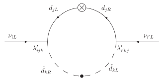
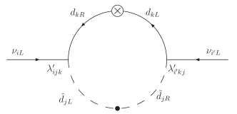
Figure 1: Feynman diagrams representing the squark-quark loop contribution to the Majorana neutrino mass.

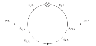
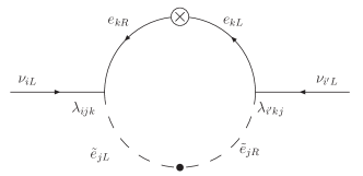
Figure 2: Feynman diagrams representing the slepton-lepton loop contribution to the Majorana neutrino mass.

Going beyond the tree level one may consider diagrams depicted on Fig. 1. The down-squark mixing is realized through the angle $\theta$. The quark mixing may be taken into account in two ways: as mixing of down-type quarks and as mixing of up-type quarks (see discussion in Ref. dedes ). Since in our case the $d$-quarks enter the loops, only their mixing will influence the results. The case of $u$-quarks mixing is equivalent to switching the mixing off and has no impact on the outcome of our calculations. We denote by $V$ the standard Cabibbo–Kobayashi–Maskawa (CKM) quark mixing matrix.

Altogether the contribution to the neutrino mass matrix coming from the squark-quark loop may be expressed as

$${\cal M}_{ii^{\prime}}^{q} = \frac{3}{16\pi^{2}}\sum_{jkl}\Bigg{\{}\left(\lambda^{\prime}_{ijk}\lambda^{\prime}_{i^{\prime}kl}\sum_{a}V_{ja}V_{la}v^{q}_{ak}m_{d^{a}}\right)$$ (25)

$$+ \left(\lambda^{\prime}_{ijk}\lambda^{\prime}_{i^{\prime}lj}\sum_{a}V_{ka}V_{la}v^{q}_{aj}m_{d^{a}}\right)\Bigg{\}},$$

where the loop integral is

$$v^{q}_{jk}=\frac{\sin 2\theta^{k}}{2}\left(\frac{\ln x_{2}^{jk}}{1-x_{2}^{jk}}-\frac{\ln x_{1}^{jk}}{1-x_{1}^{jk}}\right).$$ (26)

In the above expressions we have introduced two dimensionless quantities, $x_{1}^{jk}\equiv m_{d^{j}}^{2}/m_{\tilde{d}_{1}^{k}}^{2}$ and $x_{2}^{jk}\equiv m_{d^{j}}^{2}/m_{\tilde{d}_{2}^{k}}^{2}$. The factor 3 in Eq. (25) comes from the summation over three quark colors.

The situation is simpler for the slepton-lepton loop (Fig. 2), as the lepton mixing is much weaker and we feel justified to neglect it. By analogy with Eq. (25) we obtain

$${\cal M}_{ii^{\prime}}^{\ell}=\frac{1}{16\pi^{2}}\sum_{jk}\lambda_{ijk}\lambda_{i^{\prime}kj}(v^{\ell}_{jk}m_{e^{j}}+v^{\ell}_{kj}m_{e^{k}}),$$ (27)

with the loop integral taking the form

$$v^{\ell}_{jk}=\frac{\sin 2\phi^{k}}{2}\left(\frac{\ln y_{2}^{jk}}{1-y_{2}^{jk}}-\frac{\ln y_{1}^{jk}}{1-y_{1}^{jk}}\right),$$ (28)

where now $y_{1}^{jk}\equiv m_{e^{j}}^{2}/m_{\tilde{e}_{1}^{k}}^{2}$ and $y_{2}^{jk}\equiv m_{e^{j}}^{2}/m_{\tilde{e}_{2}^{k}}^{2}$.

The functions $v^{q}_{jk}$ and $v^{\ell}_{jk}$, which are free of $R$-parity breaking SUSY paprameters, can be calculated by running the MSSM RGE, in which the whole low energy particle/sparticle spectrum is generated. In our calculation we have used the following values for the quark sector: $m_{u}=5$ MeV, $m_{d}=9$ MeV, $m_{s}=175$ MeV, $m_{c}=1.5$ GeV, $m_{b}=5$ GeV, $m_{t}=174$ GeV, as well as the CKM matrix in the form

$$V=\begin{pmatrix}\phantom{-}0.9755&\phantom{-}0.2195&0.0031\cr-0.2201&\phantom{-}0.9746&0.0390\cr-0.0055&-0.0387&0.9989\end{pmatrix}.$$ (29)

This corresponds to the sines of quark mixing angles $s_{12}=0.2195$, $s_{23}=0.039$, and $s_{13}=0.0031$ dedes in the standard trigonometric parametrization. We have neglected the possible appearance of the CP violating phase in the quark sector.

The values of the calculated loop integrals have been arranged for clarity in the form of matrices. For the input parameters $A_{0}=100\hbox{ GeV}$, $m_{0}=m_{1/2}=150\hbox{ GeV}$, $\tan\beta=19$, $\mu>0$ we get:

$$v^{q}=\begin{pmatrix}2.361\times 10^{-4}&4.593\times 10^{-3}&1.687\times 10^{-1}\cr 2.361\times 10^{-4}&4.593\times 10^{-3}&1.687\times 10^{-1}\cr 2.358\times 10^{-4}&4.587\times 10^{-3}&1.684\times 10^{-1}\end{pmatrix},$$

$$v^{\ell}=\begin{pmatrix}6.547\times 10^{-5}&1.310\times 10^{-2}&2.528\times 10^{-1}\cr 6.547\times 10^{-5}&1.310\times 10^{-2}&2.528\times 10^{-1}\cr 6.541\times 10^{-5}&1.308\times 10^{-2}&2.525\times 10^{-1}\end{pmatrix}.$$

For the second set of parameters $A_{0}=500\hbox{ GeV}$, $m_{0}=m_{1/2}=1000\hbox{ GeV}$, $\tan\beta=19$, $\mu>0$ we find:

$$v^{q}=\begin{pmatrix}3.396\times 10^{-5}&6.606\times 10^{-4}&2.419\times 10^{-2}\cr 3.396\times 10^{-5}&6.606\times 10^{-4}&2.419\times 10^{-2}\cr 3.396\times 10^{-5}&6.605\times 10^{-4}&2.419\times 10^{-2}\end{pmatrix},$$

$$v^{\ell}=\begin{pmatrix}1.023\times 10^{-5}&2.046\times 10^{-3}&3.879\times 10^{-2}\cr 1.023\times 10^{-5}&2.046\times 10^{-3}&3.879\times 10^{-2}\cr 1.023\times 10^{-5}&2.046\times 10^{-3}&3.879\times 10^{-2}\end{pmatrix}.$$

III.2 The phenomenological neutrino mass matrix

The constraints on the various products of coupling constants $\Lambda_{i}\Lambda_{i^{\prime}}$, $\lambda_{ijk}\lambda_{i^{\prime}kj}$, and $\lambda^{\prime}_{ijk}\lambda^{\prime}_{i^{\prime}kj}$ or their values can be find by a comparison of theoretical neutrino mass matrix calculated within RpV MSSM with the phenomenological neutrino mass matrix, derived from analysis of neutrino data by making viable assumptions. It is usually done by assuming that different contributions to theoretical neutrino mass matrix do not significantly compensate each other, i.e., it is possible to extract limits on individual contributions without knowing the others.

The neutrino phenomenological mass matrix in flavor basis, ${\cal M}^{ph}$, can be written as

$${\cal M}^{ph}=U^{*}\,M^{diag}\,U^{\dagger},$$ (30)

where

$$M^{diag}\,\equiv\,diag(m_{1},\,m_{2},\,m_{3}).$$ (31)

Here $m_{i}$ are the moduli of neutrino mass eigenvalues. The three neutrino mixing scheme is assumed, namely

$$\nu_{\alpha L}\,=\,U_{\alpha i}\,\nu_{iL},~{}~{}~{}~{}~{}\alpha~{}=~{}e,\mu,\tau,~{}~{}~{}~{}i~{}=~{}1,2,3.$$ (32)

$\nu_{\alpha L}$ are flavor neutrino states and $\nu_{i}$ are the mass eigenstates.

For massive Majorana neutrinos the unitary Pontecorvo-Maki-Nakagawa-Sakata (PMNS) matrix $U$ in the standard parameterization has the form

$$U=\left(\begin{array}[]{ccc}c_{12}c_{13}&s_{12}c_{13}&s_{13}e^{-i\delta}\\ -s_{12}c_{23}-c_{12}s_{23}s_{13}e^{i\delta}&c_{12}c_{23}-s_{12}s_{23}s_{13}e^{i\delta}&s_{23}c_{13}\\ s_{12}s_{23}-c_{12}c_{23}s_{13}e^{i\delta}&-c_{12}s_{23}-s_{12}c_{23}s_{13}e^{i\delta}&c_{23}c_{13}\end{array}\right)\left(\begin{array}[]{ccc}1&0&0\\ 0&e^{i\alpha_{12}}&0\\ 0&0&e^{i\alpha_{13}}\end{array}\right),$$ (39)

where $s_{ij}\equiv\sin\theta_{ij}$, $c_{ij}\equiv\cos\theta_{ij}$. Three mixing angles $\theta_{ij}$ ($i<j$) vary between 0 and $\pi/2$. The $\delta$ is the CP violating Dirac phase and $\alpha_{12}$, $\alpha_{13}$ are CP violating Majorana phases. Their values vary between $0$ and $2\pi$. The expression for ${\cal M}^{ph}_{\alpha\beta}$ in terms of $m_{i}$, $\theta_{ij}$, $\delta$, $\alpha_{12}$, $\alpha_{13}$ is given in the Appendix.

The analysis of the Super-Kamiokande atmospheric neutrino data SK and the global analysis of the data of the solar neutrino experiments and KamLAND experiment Kamland yield the following best fit values of the relevant neutrino oscillation parameters:

$$\Delta m^{2}_{23} = 2.1\times 10^{-3}~{}\hbox{ eV}^{2},~{}~{}~{}~{}~{}~{}\sin^{2}2\theta_{23}~{}=~{}1.00,$$

$$\Delta m^{2}_{12} = 7.1\times 10^{-5}~{}\hbox{ eV}^{2},~{}~{}~{}~{}~{}~{}\tan^{2}\theta_{12}~{}=~{}0.40.$$

The neutrino mass-squared difference is determined as $\Delta m^{2}_{ik}~{}=~{}m^{2}_{k}-m^{2}_{i}$. For the angle $\theta_{13}$ only the upper bound is known. From exclusion plot obtained from the data of the reactor experiment CHOOZ CHOOZ we have

$$\sin^{2}\theta_{13}\,\leq\,5\times 10^{-2}~{}~{}~{}~{}~{}~{}(90\%\ \rm{c.l.}).$$ (41)

The CP violating phases $\delta$, $\alpha_{12}$ and $\alpha_{13}$ remain undetermined.

Neutrino oscillation data are insensitive to the absolute scale of neutrino masses. The values of neutrino masses depend on the lightest neutrino mass, on the neutrino mass spectrum and the neutrino mass-squared differences $\Delta m^{2}_{12}$ and $\Delta m^{2}_{23}$. The neutrino oscillation data are compatible with two types of neutrino mass spectra:
i) The normal hierarchy (NH) mass spectrum, which corresponds to the case

$$m_{1}~{}\ll~{}m_{2}~{}\ll~{}m_{3}.$$ (42)

ii) The inverted hierarchy (IH) of neutrino masses. It is given by the condition

$$m_{3}~{}\ll~{}m_{1}~{}<~{}m_{2}.$$ (43)

The $0\nu\beta\beta$-decay is one of the most sensitive known ways to probe the absolute values of neutrino masses and the type of the spectrum. The most stringent lower bound on the half-life of $0\nu\beta\beta$-decay were obtained in the Heidelberg-Moscow ⁷⁶Ge experiment H-M ($T^{0\nu-exp}_{1/2}\geq 1.9\times 10^{25}$ yr). By assuming the nuclear matrix element of Ref. FedorVogel we end up with $|m_{\beta\beta}|=U^{2}_{e1}\,m_{1}+U^{2}_{e2}\,m_{2}+U^{2}_{e3}\,m_{3}\leq 0.55\hbox{ eV}$, where $U$ is the neutrino mixing matrix Eq. (39). With this input limit we can find the maximal allowed values for the matrix elements ${\cal M}^{ph}_{ij}$ of the neutrino mass matrix, which are as follows:

$$|{\cal M}^{ph-HM}|\leq\left(\begin{array}[]{ccc}0.55&1.29&1.29\\ 1.29&1.35&1.04\\ 1.29&1.04&1.35\end{array}\right)~{}\hbox{ eV}.$$ (47)

In the calculation we used best fit values of mass-squared differences $\Delta m^{2}_{12}$, $\Delta m^{2}_{23}$ and mixing angles $\theta_{12}$, $\theta_{23}$ SK ; Kamland : $\sin^{2}\theta_{13}=[0,5\times 10^{-2}]$, $\delta,~{}\alpha_{12},\alpha_{13}~{}=~{}[0,2\pi]$ and the whole allowed mass parameter space of neutrinos was taken into account.

The phenomenological neutrino mass matrix can be constructed from the assumption of normal or inverted hierarchy of neutrino masses. If mass squared-differences and mixing angles of (LABEL:bestfit) and (41) are considered we obtain

$$|{\cal M}^{ph-IH}|=10^{-2}~{}\hbox{ eV}$$

$$\times\left(\begin{array}[]{ccc}(1.80,4.52)&(0.025,3.12)&(0.025,3.12)\\ (0.025,3.12)&(0.028,2.40)&(0.945,2.39)\\ (0.025,3.12)&(0.945,2.39)&(0.028,2.40)\end{array}\right),$$

$$|{\cal M}^{ph-NH}|=10^{-4}~{}\hbox{ eV}$$

$$\times\left(\begin{array}[]{ccc}(0.53,45.2)&(26.9,98.9)&(26.9,98.9)\\ (26.9,98.9)&(173,254)&(182,254)\\ (26.9,98.9)&(182,254)&(173,254)\end{array}\right).$$

Here, we assumed that the mass of the lightest neutrino is negligible. The allowed ranges have origin in the uncertainty coming from the $\theta_{13}$ parameter and the CP violating phases.

III.3 The magnetic moments of neutrinos

Once neutrinos are massive, they can have magnetic moments. We distinguish magnetic moments of Dirac and Majorana neutrinos:
i) The Dirac magnetic moment, which connects left-handed electroweak doublet neutrino $\nu_{iL}$ to a right-handed electroweak singlet neutrino $\nu_{jR}$ ($i,j=e,~{}\mu,~{}\tau$). One can express the effective Hamiltonian, which conserves the total lepton number, as

$$H^{D}_{\rm eff}=\frac{1}{2}\mu^{D}_{\nu_{ij}}\bar{\nu}_{iL}\sigma^{\alpha\beta}\nu_{jR}F_{\beta\alpha}+{\rm h.c.},$$ (50)

where $\mu_{\nu^{D}_{ij}}$ is Dirac diagonal ($i=j$) or transition ($i\neq j$) magnetic moment between states $\nu_{iL}$ and $\nu_{jR}$.

A minimal extension of the SM with a right-handed singlet neutrino yields a diagonal neutrino magnetic moment of marci

$$\mu_{\nu}=\frac{3}{4\pi^{2}}\frac{G_{F}m_{e}m_{\nu}}{\sqrt{2}}\mu_{B}.$$ (51)

Here, $\mu_{B}=e/(2m_{e})$ is the Bohr magneton and $m_{\nu}$ is the neutrino mass. By using the neutrino oscillation data one finds $\mu_{\nu}\geq 4\times 10^{-20}~{}\mu_{B}$. It is believed that larger values of magnetic moment are possible in extensions of the SM, e.g., in models with large extra dimensions edmoh . A neutrino magnetic moment $\mu_{\nu}$ of the order of $10^{-11}~{}\mu_{B}$ might be an explanation of solar neutrino problem by flipping $\nu_{e}$ to sterile neutrinos volo ; barb ; grimus ; senja ; jvns ; bala .

ii) The Majorana magnetic moment acts between neutrino fields of the same chirality, namely $\nu_{iL}$ and $\nu_{jL}^{c}$ As a consequence it violates the total lepton number by two units ($\Delta L=2$). The effective Hamiltonian takes the form

$$H^{M}_{\rm eff}=\frac{1}{2}\mu^{M}_{ij}\bar{\nu}_{iL}\sigma^{\alpha\beta}\nu_{jL}^{c}F_{\beta\alpha}+{\rm h.c.}$$ (52)

Majorana neutrinos cannot possess a flavour diagonal ($i=j$) magnetic moment due to the CPT theorem. They can have only transition ($i\neq j$) magnetic moment mmmn . From the definition one sees that $\mu_{\nu_{ij}}$ vanishes for $i=j$ and also that magnetic moment is antisymmetric in indices $i,j$: $\mu_{\nu_{ij}}=-\mu_{\nu_{ji}}$.

The limits on neutrino transition magnetic moments arise from laboratory measurements of the $\nu_{e}-e$ scattering cross section using solar, atmospheric and terrestrial neutrinos nmmlim . These experiments have put upper bounds on $\mu^{D}_{\nu_{ij}}$, which are as follows:

$$\mu^{D}_{\nu_{ej}} \leq 0.9\times 10^{-10}~{}\mu_{B},$$

$$\mu^{D}_{\nu_{\mu j}} \leq 6.8\times 10^{-10}~{}\mu_{B},$$

$$\mu^{D}_{\nu_{\tau j}} \leq 3.9\times 10^{-7}~{}\mu_{B}.$$ (53)

The most restrictive limits remains those from the atrophysical analysis of the energy-loss rate of stars due to the $\gamma\rightarrow\nu\overline{\nu}$ process, which are raff

$$\mu^{D}_{\nu_{ij}}\leq 3\times 10^{-12}~{}\mu_{B}.$$ (54)

The assumption is that this energy loss mechanism of giant red stars cannot exceed energy loss via weak processes. For Majorana transition magnetic moments $\mu^{M}_{\nu_{ij}}$ the above limits are twice stronger sacha .

The cases of Dirac and Majorana magnetic moments have fundamentally different physical applications and need to be considered separately. In this paper we assume massive neutrinos to be Majorana particles. In addition, we shall take advantage of the fact that neutrino magnetic moments have an intimate connection to their masses, which is model dependent. Recently, the contribution of transition magnetic moments to the neutrino mass matrix was estimated in sacha . It was found that if neutrino transition magnetic moments are of the order of their current upper bound, their contribution to ${\cal M}_{ij}$ can exceed the experimental value of ${\cal M}^{ph}_{ij}$. The purpose of this paper is to discuss the impact of the ${\cal M}^{ph}_{ij}$ on the transition magnetic moments of Majorana neutrinos within the GUT constrained MSSM with explicit $R$-parity violation.

In order to generate the magnetic moments within the $R$-parity breaking SUSY one needs to attach a photon to one of the internal lines in the loops from Figs. 1 and 2. For each Feynman diagram we have two possibilities. One can attach the photon to quark (lepton) or squark (slepton) internal line of the loop. However, the contributions coming from photon–sparticle interactions are suppressed by big masses of the latter and we may safely ignore them.

The contribution coming from the squark–quark loop takes again into account squark and quark mixing. We end up with

$$\mu_{\nu_{ii^{\prime}}}^{q} = (1-\delta_{ii^{\prime}})\frac{12Q_{d}m_{e}}{16\pi^{2}}\sum_{jkl}\Bigg{\{}\lambda^{\prime}_{ijk}\lambda^{\prime}_{i^{\prime}kl}\sum_{a}V_{ja}V_{la}\frac{w^{q}_{ak}}{m_{d^{a}}}$$ (55)

$$- \lambda^{\prime}_{ijk}\lambda^{\prime}_{i^{\prime}lj}\sum_{a}V_{ka}V_{la}\frac{w^{q}_{aj}}{m_{d^{a}}}\Bigg{\}}\mu_{B},$$

where now the loop integral takes a slightly more complicated form

$$w^{q}_{jk}=\frac{\sin 2\theta^{k}}{2}\left(\frac{x_{2}^{jk}\ln x_{2}^{jk}-x_{2}^{jk}+1}{(1-x_{2}^{jk})^{2}}-(x_{2}\to x_{1})\right).$$ (56)

Here $Q_{d}=1/3$ is the $d$-quark charge in units of $e$, and $m_{e}$ denotes the electron mass. We work in mathematical units, ie. we set $\hbar=1$. We note that the resulting formula is antisymmetric as expected.

The contribution from the slepton–lepton loop reads

$$\mu_{\nu_{ii^{\prime}}}^{\ell} = (1-\delta_{ii^{\prime}})\frac{4Q_{e}m_{e}}{16\pi^{2}}$$

$$\times \sum_{jk}\lambda_{ijk}\lambda_{i^{\prime}kj}\left(\frac{w^{\ell}_{jk}}{m_{e^{j}}}-\frac{w^{\ell}_{kj}}{m_{e^{k}}}\right)\mu_{B}$$

where the loop integral is as previously equal to

$$w^{\ell}_{jk}=\frac{\sin 2\phi^{k}}{2}\left(\frac{y_{2}^{jk}\ln y_{2}^{jk}-y_{2}^{jk}+1}{(1-y_{2}^{jk})^{2}}-(y_{2}\to y_{1})\right).$$ (58)

It is worthwhile to notice that if quark mixing is neglected, $\sin{2\theta^{k}}/2\approx m_{d^{k}}m_{\tilde{d}^{k}}/(m_{\tilde{d}_{1}^{k}}^{2}-m_{\tilde{d}_{2}^{k}}^{2})$ and the masses of squarks $m_{\tilde{d}_{1}^{k}}$, $m_{\tilde{d}_{2}^{k}}$ are replaced with their average value $m_{\tilde{d}^{k}}$, the expression for $\mu_{\nu_{ii^{\prime}}}^{q}$ of Ref. Bhatta is reproduced. The same procedure allows to obtain the result of Bhatta also for $\mu_{\nu_{ii^{\prime}}}^{\ell}$. In this case $\sin{2\phi^{k}}/2\approx m_{e^{k}}m_{\tilde{e}^{k}}/(m_{\tilde{e}_{1}^{k}}^{2}-m_{\tilde{e}_{2}^{k}}^{2})$ and $m_{\tilde{e}_{1}^{k}}$, $m_{\tilde{e}_{2}^{k}}$ = $m_{\tilde{e}^{k}}$ (the average mass of sleptons) have to be considered.

Table 1: The SUSY coefficients converting elements of neutrino mass mass matrix to transition magnetic moments of Majorana neutrinos (see Eqs. (59) and (60) for definition). It is assumed $\mu>0$.

SUSY input				The SUSY conversion coefficient
$A_{0}$	$m_{0}$	$m_{1/2}$	$\tan\beta$	$f^{q}_{\rm SUSY}$	$f^{q-CKM}_{\rm SUSY}$	$f^{\ell}_{\rm SUSY}$
$[\hbox{ GeV}]$	$[\hbox{ GeV}]$	$[\hbox{ GeV}]$		$[\hbox{ eV}^{-1}]$	$[\hbox{ eV}^{-1}]$	$[\hbox{ eV}^{-1}]$
100	150	150	5	$(0.3,1.0)\times 10^{-16}$	$(2.8,8.8)\times 10^{-17}$	$(0.5,1.5)\times 10^{-15}$
			19	$(0.3,1.2)\times 10^{-16}$	$(2.8,9.8)\times 10^{-17}$	$(0.5,1.6)\times 10^{-15}$
500	1000	1000	5	$(1.1,2.8)\times 10^{-18}$	$(1.0,2.4)\times 10^{-18}$	$(1.7,4.1)\times 10^{-17}$
			19	$(1.1,3.1)\times 10^{-18}$	$(1.0,2.7)\times 10^{-18}$	$(1.7,4.3)\times 10^{-17}$

Table 2: The Majorana neutrino transition magnetic moment $\mu_{\nu_{ij}}$ ($ij=e\mu,~{}e\tau,~{}\mu\tau$) derived from phenomenological mass matrices (see text for details). The upper bounds on magnetic moments are obtained by using the current neutrino oscillation and the $0\nu\beta\beta$-decay data. The predictions for $\mu_{\nu_{ij}}$ were calculated by assuming the inverted hierarchy or the normal hierarchy of neutrino masses and that the lightest neutrino is massless. The ranges of allowed values correspond to uncertainty in SUSY coefficient $f^{q,l}_{SUSY}$ and in CP-violating violating phases. Two different GUT scenarios are considered. The remaining SUGRA parameters are $\tan\beta=19$ and $\mu>0$. $\mu_{B}$ is the Bohr magneton.

SUSY input in GeV			Transition magnetic moment $\mu_{\nu_{ij}}$ in $\mu_{B}$
$A_{0}$	$m_{0}$	$m_{1/2}$	$ij$	$0\nu\beta\beta$ constraints	inverted hierarchy	normal hierarchy
				lepton-slepton loop mechanism
100	150	150	$e\mu,e\tau$	$\leq(0.62,2.10)\times 10^{-15}$	$(0.01,5.00)\times 10^{-17}$	$(0.13,1.60)\times 10^{-17}$
			$\mu\tau$	$\leq(0.50,1.70)\times 10^{-15}$	$(0.45,3.80)\times 10^{-17}$	$(0.87,4.10)\times 10^{-17}$
500	1000	1000	$e\mu,e\tau$	$\leq(2.20,5.50)\times 10^{-17}$	$(0.04,13.0)\times 10^{-19}$	$(0.47,4.20)\times 10^{-19}$
			$\mu\tau$	$\leq(1.80,4.50)\times 10^{-17}$	$(0.16,1.00)\times 10^{-18}$	$(0.32,1.10)\times 10^{-18}$
				quark-squark loop mechanism (without d-quarks mixing)
100	150	150	$e\mu,e\tau$	$\leq(0.41,1.50)\times 10^{-16}$	$(0.08,36.0)\times 10^{-19}$	$(0.08,1.10)\times 10^{-18}$
			$\mu\tau$	$\leq(0.33,1.20)\times 10^{-16}$	$(0.30,2.80)\times 10^{-18}$	$(0.58,3.00)\times 10^{-18}$
500	1000	1000	$e\mu,e\tau$	$\leq(1.40,4.00)\times 10^{-18}$	$(0.03,9.60)\times 10^{-20}$	$(0.30,3.00)\times 10^{-20}$
			$\mu\tau$	$\leq(1.20,3.20)\times 10^{-18}$	$(1.00,7.30)\times 10^{-20}$	$(2.00,7.80)\times 10^{-20}$
				quark-squark loop mechanism (with d-quarks mixing)
100	150	150	$e\mu,e\tau$	$\leq(0.36,1.30)\times 10^{-16}$	$(0.07,31.0)\times 10^{-19}$	$(0.76,9.70)\times 10^{-19}$
			$\mu\tau$	$\leq(0.29,1.00)\times 10^{-16}$	$(0.27,2.30)\times 10^{-18}$	$(0.51,2.50)\times 10^{-18}$
500	1000	1000	$e\mu,e\tau$	$\leq(1.30,3.40)\times 10^{-18}$	$(0.03,8.30)\times 10^{-20}$	$(0.28,2.60)\times 10^{-20}$
			$\mu\tau$	$\leq(1.10,2.80)\times 10^{-18}$	$(0.97,6.40)\times 10^{-20}$	$(1.90,6.80)\times 10^{-20}$

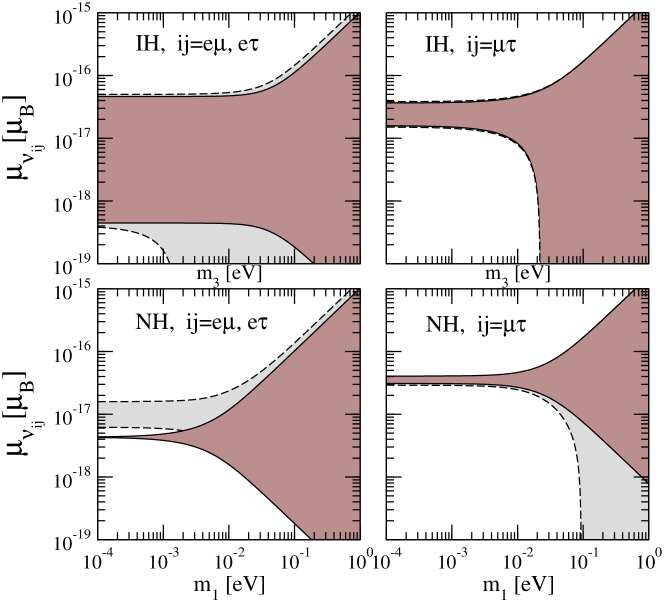
Figure 3: Transition magnetic moments of Majorana neutrinos $\mu_{\nu_{e\mu}}$, $\mu_{\nu_{e\tau}}$ and $\mu_{\nu_{\mu\tau}}$ as function of the lightest neutrino mass $m_{3}$ (the inverted hierarchy of neutrino masses, upper panels) and $m_{1}$ (the normal hierarchy of neutrino masses, lower panels). The results are presented for $\sin^{2}\theta_{13}=0$ (the region with solid line boundaries) and $\sin^{2}\theta_{13}=5\times 10^{-2}$ (the region with dashed line boundaries). In the calculation the best fit values of mass-squared differences $\Delta m^{2}_{12}$, $\Delta m^{2}_{23}$ and mixing angles $\theta_{12}$, $\theta_{23}$ were considered SK ; Kamland . For CP-violating phase we assumed $\delta,~{}\alpha_{12},\alpha_{13}~{}=~{}[0,2\pi]$. The largest value of the SUSY coefficient $f^{q,l}_{SUSY}$ for the set of SUSY parameters $(A_{0}=100\hbox{ GeV}$, $m_{0}=m_{1/2}=150\hbox{ GeV})$, $\tan\beta=19$ and $\mu>0$ was taken into account. IH and NH denote the inverted hierarchy and the normal hierarchy of neutrino masses, respectively. $\mu_{B}$ is the Bohr magneton.

The matrices $w^{q}_{jk}$ and $w^{\ell}_{jk}$ in flavor space are evaluated for two representative sets of input parapeters $A_{0}$, $m_{0}$, $m_{1/2}$, $\tan\beta$ and $\mu>0$. By assuming $A_{0}=100\hbox{ GeV}$, $m_{0}=m_{1/2}=150\hbox{ GeV}$, $\tan\beta=19$, $\mu>0$ we end up with

$$w^{q}=\begin{pmatrix}2.582\times 10^{-12}&5.024\times 10^{-11}&2.332\times 10^{-9}\cr 6.759\times 10^{-10}&1.315\times 10^{-8}&6.068\times 10^{-7}\cr 2.750\times 10^{-7}&5.350\times 10^{-6}&2.421\times 10^{-4}\end{pmatrix},$$

$$w^{\ell}=\begin{pmatrix}1.223\times 10^{-14}&2.446\times 10^{-12}&5.163\times 10^{-11}\cr 2.691\times 10^{-10}&5.384\times 10^{-8}&1.132\times 10^{-6}\cr 4.832\times 10^{-8}&9.668\times 10^{-6}&2.019\times 10^{-4}\end{pmatrix}.$$

If larger SUSY mass scale is assumed with $A_{0}=500\hbox{ GeV}$, $m_{0}=m_{1/2}=1000\hbox{ GeV}$, $\tan\beta=19$, $\mu>0$, we obtain

$$w^{q}=\begin{pmatrix}9.895\times 10^{-15}&1.925\times 10^{-13}&8.809\times 10^{-12}\cr 2.780\times 10^{-12}&5.408\times 10^{-11}&2.466\times 10^{-9}\cr 1.383\times 10^{-9}&2.690\times 10^{-8}&1.216\times 10^{-6}\end{pmatrix},$$

$$w^{\ell}=\begin{pmatrix}5.316\times 10^{-17}&1.064\times 10^{-14}&2.126\times 10^{-13}\cr 1.301\times 10^{-12}&2.602\times 10^{-10}&5.195\times 10^{-9}\cr 2.755\times 10^{-10}&5.511\times 10^{-8}&1.098\times 10^{-6}\end{pmatrix}.$$

IV Results

The main purpose of our present work is to calculate the transition magnetic moments for Majorana neutrinos. To achieve this goal one proceeds as follows. First one finds the values of the loop integrals $v^{\ell}$, $v^{q}$, $w^{\ell}$ and $w^{q}$ within some GUT scenario. We have chosen two sets of parameters: $(A_{0}=100\hbox{ GeV},m_{0}=m_{1/2}=150\hbox{ GeV})$ and $(A_{0}=500\hbox{ GeV},m_{0}=m_{1/2}=1000\hbox{ GeV})$, in both of them keeping $\tan\beta=19$ and positive $\mu$. This allows us to construct the theoretical mass matrices, Eqs. (25) and (27), and confront them with phenomenological ones. Next we calculate the contributions from the $\ell$–loop and the $q$–loop. The crucial point is that we consider each mechanism separately, which means that only one element from the sums in Eqs. (25) and (27) is picked up at a time. Such approach is justified by the usual assumption that there is no fine-tuning between different contributions, which therefore may by analyzed separately. Explicitly, the simplified expressions read:

$$\mu_{\nu_{ii^{\prime}}}^{q} \simeq (1-\delta_{ii^{\prime}})\frac{4}{3}\mu_{B}m_{e^{1}}{\cal M}^{q}_{ii^{\prime}}\left[\frac{\displaystyle{\sum_{a}V_{ja}V_{la}w^{q}_{ak}/m_{q^{a}}}}{\displaystyle{\sum_{a}V_{ja}V_{la}v^{q}_{ak}m_{q^{a}}}}\right]_{\rm max}$$ (59)

$$\equiv (1-\delta_{ii^{\prime}}){\cal M}^{q}_{ii^{\prime}}f^{q}_{\rm SUSY},$$

$$\mu_{\nu_{ii^{\prime}}}^{\ell} \simeq (1-\delta_{ii^{\prime}})4\mu_{B}m_{e^{1}}{\cal M}^{\ell}_{ii^{\prime}}\left[\frac{\displaystyle{w^{\ell}_{jk}/m_{e^{j}}}}{\displaystyle{v^{\ell}_{jk}m_{e^{j}}}}\right]_{\rm max}$$ (60)

$$\equiv (1-\delta_{ii^{\prime}}){\cal M}^{q}_{ii^{\prime}}f^{\ell}_{\rm SUSY},$$

where the $[...]_{\rm max}$ symbol denotes that we have checked all the combinations of indices $\{j,k,l\}$ in the first case and $\{j,k\}$ in the second one, and picked up the dominant mechanism.

The coefficients $f^{\ell,q}_{\rm SUSY}$ convert the neutrino masses into magnetic moments. We list their values, obtained for four different sets of GUT parameters, in Tab. 1. The $f^{q-CKM}_{\rm SUSY}$ parameter takes into account quark mixing, which is absent in $f^{q}_{\rm SUSY}$. This additional mechanism slightly lowers the maximal allowed value of the magnetic moment One sees also that the dependence on the $\tan\beta$ parameter is very weak, therefore in the following we will discuss only the case of large $\tan\beta=19$. For completeness we include also in the table the lower bounds on the $f$ coefficients, which were obtained by finding the smallest of the expressions in square brackets in Eqs. (59) and (60).

The resulting values of $\mu_{\nu_{ii^{\prime}}}$ for six different scenarios are presented in Tab. 2. Due to antisymmetricity the diagonal elements $\mu_{\nu_{ii}}$ are zero. The ranges of values in the first column are the highest upper limit and lowest upper limit on the transition magnetic moment, coming from different mechanisms (different combination of coupling constants $\lambda\lambda$ or $\lambda^{\prime}\lambda^{\prime}$). They were calculated using the ${\cal M}^{ph-HM}$ mass matrix. One clearly sees that in this case the different mechanisms give comparable results. However, the imposed GUT constraints have a much bigger impact and introduce two orders of magnitude differences. The values from the first column for the first set of GUT parameters ($A_{0}=100\hbox{ GeV}$, $m_{0}=m_{1/2}=150\hbox{ GeV}$) may be roughly compared with the predictions published in Ref. Bhatta showing that for this special case we our results are compatible with the previously published.

The two remaining columns present the ranges of allowed values of the magnetic moments if one assumes normal or inverted mass hierarchy of the neutrinos. These results take into account various mechanisms of generating $\mu_{\nu_{ii^{\prime}}}$ as well as the experimental uncertainties shown in mass matrices ${\cal M}^{ph-IH}$ and ${\cal M}^{ph-NH}$. In this case the ranges span roughly over 1–2 orders of magnitude. It is visible that, regardless of the GUT parameters, one should not expect the magnetic moment to be greater than $10^{-17}\mu_{B}$, which is not possible to detect experimentally nowadays.

It is interesting to investigate the influence of quark mixing on the results. When quark mixing is switched off, the maximal allowed $\mu^{q}_{\nu}$ values drop down approximately by 10 to 20%.

In the case when the lightest neutrino mass is not set to zero, one may express all the remaining mass eigenstates in terms of $m_{1(3)}$ and appropiate differences of masses squared, which are known from the results of the neutrino oscillation experiments. On Fig. 3 we present the allowed values for different elements of the neutrino mass matrix as the function of $m_{1(3)}$ in the case of NH and IH. The shaded regions correspond to all possible combinations of the two Majorana $\alpha_{12}$ and $\alpha_{13}$, and one Dirac phase $\delta$, for $\sin^{2}\theta_{13}=0$ (dark shading) and $\sin^{2}\theta_{13}\leq 0.05$ (lighter shading). One sees clearly, that the phase factors as well as possible non-zero mass of lightest neutrino modify the results in a non-trivial fashion.

V Summary

Since the neutrinos have no electric charge they can be Majorana fermions. A Majorana neutrino is more natural than a Dirac neutrino as it allows to explain the smallness of their masses in theories with grand unification. Majorana neutrinos have zero diagonal magnetic moments while they may in general have transition magnetic moments $\mu_{\nu_{ij}}$ ($i\neq j$). The question is, how large they are? In this paper we studied this issue within the GUT constrained MSSM with explicit $R$-parity violation.

The transition magnetic moments were induced by attaching photons to the internal lines of lepton-slepton and quark-squarks loop diagrams that generate neutrino masses. $\mu_{\nu_{ij}}$ has been written as a product of SUSY conversion coefficients $f_{SUSY}$, which reflects the dependence on SUSY parameter space and quark mixing, and the element of Majorana neutrino mass matrix in flavor basis.

Two possible GUT scenarios were considered: $A_{0}=100\hbox{ GeV}$, $m_{0}=m_{1/2}=150\hbox{ GeV}$, and $A_{0}=500\hbox{ GeV}$, $m_{0}=m_{1/2}=1000\hbox{ GeV}$, in both of them having $\tan\beta=19$ and positive $\mu$ parameter. Our study showed that $f_{SUSY}$ is nearly insensitive on the value of $\tan\beta$ and that its dependence on the scale of GUT common mass and coupling constants parameters $m_{0}$, $m_{1/2}$, and $A_{0}$ dominates. The difference in $f_{SUSY}$ for these two scenarios reach around two orders of magnitude. It is worth mentioning that contributions to $\mu_{\nu_{ij}}$ from lepton-slepton mechanisms dominates over contributions from quark-squark diagrams.

The transition magnetic moments were calculated by considering three differently constructed phenomenological neutrino mass matrices. The elements of the first one (${\cal M}^{ph-HM}$) represent the maximal allowed values, if neutrino oscillation data SK ; Kamland and the lower bound on the $0\nu\beta\beta$-decay half-life of ⁷⁶Ge H-M are taken into account. The corresponding upper limits on $\mu_{\nu_{e\mu}}$, $\mu_{\nu_{e\tau}}$ and $\mu_{\nu_{\mu\tau}}$ have been found to be of the order of $10^{-15}~{}\mu_{B}$ and $10^{-17}~{}\mu_{B}$ for the assumed two SUSY scenarios.

Two phenomenological neutrino mass matrices were generated by considering normal and inverted hierarchy of neutrino masses and that the mass of the lightest neutrino is zero. This allowed to make predictions for transition magnetic moments of Majorana neutrinos. For low (large) SUSY parameter scale we found the maximal value $5\times 10^{-17}~{}\mu_{B}$ ($1.3\times 10^{-18}~{}\mu_{B}$). The dependence of the results on the neutrino mass pattern is weak.

The magnetic moments $\mu_{\nu_{e\mu}}$, $\mu_{\nu_{e\tau}}$ and $\mu_{\nu_{\mu\tau}}$ were calculated also as a function of the lightest neutrino mass. The best fit values of neutrino oscillation parameters were considered. Only for the mixing angle $\theta_{13}$ it was assumed $\sin^{2}\theta_{13}=0$ and $\sin^{2}\theta_{13}=5\times 10^{-2}$. It is worth mentioning that the maximal mixing of atmospheric neutrinos ($\theta_{23}=\pi/4$) implies that the allowed ranges of $\mu_{\nu_{e\mu}}$ and $\mu_{\nu_{e\tau}}$ are the same, if the Dirac and Majorana CP violating phases vary from 0 to $\pi/2$. The results show that especially $\mu_{\nu_{e\mu,e\tau}}$ (inverted hierachy of neutrino masses) depends strongly on the values of CP phases.

The obtained results show that the values of the Majorana transition magnetic moments might be significantly above the scale of the Dirac-type magnetic moment in minimal extension of the SM with right-handed neutrinos. However, the maximal values are still too small to be tested in the present laboratory experiments or to have astrophysical consequences.

Acknowledgments This work was supported by the VEGA Grant agency of the Slovak Republic under contract No. 1/3039/06, by the EU ILIAS project under contract RII3-CT-2004-506222, by the DFG project 436 SLK 17/298 and the Polish State Committee for Scientific Research under grants no. 2P03B 071 25 and 1P03B 098 27. One of us (MG) greatly acknowledges the financial support from the Foundation for Polish Science.

VI Appendix

In this appendix, for covenience of the reader we present explicit expressions for the neutrino mass matrix in flavor basis, ${\cal M}_{\alpha\beta}$ ($\alpha,\beta=e,\mu,\tau$), as functions of the moduli of neutrino mass eigenvalues $m_{i}$, of mixing angles $\theta_{ij}$ and of the CP violating phases $\delta$, $\alpha_{12}$, $\alpha_{13}$ frigerio . The matrix element ${\cal M}$ is symmetric, i.e., it is defined by six elements:

$${\cal M}_{ee} = ~{}~{}c_{13}^{2}\,c_{12}^{2}\,{m_{1}}\,+\,c_{13}^{2}\,s_{12}^{2}\,{m_{2}}\,{e^{-i2\alpha_{{}_{12}}}}\,+\,s_{13}^{2}\,{e^{2\,i\delta}}\,{m_{3}}\,{e^{-i2\alpha_{{}_{13}}}},$$

$${\cal M}_{e\mu} = -\,c_{12}\,c_{13}\,\left(\,c_{23}\,s_{12}\,+\,c_{12}\,s_{23}\,s_{13}\,{e^{-i\delta}}\,\right){\it{m_{1}}}$$

$$+\,c_{13}\,s_{12}\left(\,c_{23}\,c_{12}\,-\,s_{23}\,s_{12}\,s_{13}\,{e^{-i\delta}}\right)\,{\it{m_{2}}}\,{e^{-i2\alpha_{{}_{12}}}}\,+\,c_{13}\,s_{23}\,s_{13}\,{e^{i\delta}}\,{m_{3}}\,{e^{-i2\alpha_{{}_{13}}}},$$

$${\cal M}_{e\tau} = -\,c_{12}\,c_{13}\,\left(-\,s_{23}\,s_{12}\,+\,c_{23}\,c_{12}\,s_{13}\,{e^{-i\delta}}\right)\,{m_{1}}$$

$$-\,c_{13}\,s_{12}\,\left(\,c_{12}\,s_{23}\,+\,c_{23}\,s_{12}\,s_{13}\,{e^{-i\delta}}\,\right){m_{2}}{e^{-i2\alpha_{{}_{12}}}}\,+\,c_{23}\,c_{13}\,s_{13}\,{e^{i\delta}}\,{m_{3}}\,{e^{-i2\alpha_{{}_{13}}}},$$

$${\cal M}_{\mu\mu} = ~{}~{}\left(c_{23}^{2}\,s_{12}^{2}\,+\,2\,c_{23}\,c_{12}\,s_{23}\,s_{12}\,s_{13}\,{e^{-i\delta}}\,+c_{12}^{2}\,s_{23}^{2}\,s_{13}^{2}\,{e^{-2i\,\delta}}\right)\,m_{1}\,$$

$$+\left(c_{23}^{2}\,c_{12}^{2}\,-\,2\,c_{23}\,c_{12}\,s_{23}\,s_{12}\,s_{13}\,{e^{-i\delta}}\,+\,s_{23}^{2}\,s_{12}^{2}\,s_{13}^{2}\,{e^{-2i\,\delta}}\right)\,{m_{2}}\,{e^{-i2\alpha_{{}_{12}}}}\,+\,c_{13}^{2}\,s_{23}^{2}\,{m_{3}}\,{e^{-i2\alpha_{{}_{13}}}},$$

$${\cal M}_{\mu\tau} = -\left(c_{23}\,s_{23}\,s_{12}^{2}\,-\,c_{23}^{2}\,c_{12}\,s_{12}\,s_{13}\,{e^{-i\delta}}\,+\,c_{12}\,s_{23}^{2}\,s_{12}\,s_{13}\,{e^{-i\delta}}\,-\,c_{23}\,c_{12}^{2}\,s_{23}\,s_{13}^{2}\,{e^{-2\,i\delta}}\,\right){\it{m_{1}}}$$

$$-\left(c_{23}\,c_{12}^{2}\,s_{23}\,+\,c_{23}^{2}\,c_{12}\,s_{12}\,s_{13}\,{e^{-i\delta}}\,-\,c_{12}\,s_{23}^{2}\,s_{12}\,s_{13}\,{e^{-i\delta}}\,-\,c_{23}\,s_{23}\,s_{12}^{2}\,s_{13}^{2}\,{e^{-2\,i\delta}}\,\right)\,{m_{2}}\,{e^{-i2\alpha_{{}_{12}}}}$$

$$\,+\,c_{23}\,c_{13}^{2}\,s_{23}\,{m_{3}}\,{e^{-i2\alpha_{{}_{13}}}},$$

$${\cal M}_{\tau\tau} = ~{}~{}\left(s_{23}^{2}\,s_{12}^{2}\,-\,2\,c_{23}\,c_{12}\,s_{23}\,s_{12}\,s_{13}\,{e^{-i\delta}}\,+\,c_{23}^{2}\,c_{12}^{2}\,s_{13}^{2}\,{e^{-2\,i\delta}}\right){m_{1}}$$

$$+\left(c_{12}^{2}\,s_{23}^{2}\,+\,2\,c_{23}\,c_{12}\,s_{23}\,s_{12}\,s_{13}\,{e^{-i\delta}}+c_{23}^{2}\,s_{12}^{2}\,s_{13}^{2}\,{e^{-2\,i\delta}}\right)\,{m_{2}}\,{e^{-i2\alpha_{{}_{12}}}}\,+\,c_{23}^{2}\,c_{13}^{2}\,{m_{3}}\,{e^{-i2\alpha_{{}_{13}}}}.$$

The maximal mixing of atmospheric neutrinos ($\theta_{23}=\pi/4$) implies symmetry among some of elements of the neutrino mass matrix ${\cal M}_{\alpha\beta}$. If CP-violating phases are considered as free parameters the allowed ranges of $|{\cal M}_{e\mu}|$ and $|{\cal M}_{e\tau}|$ ($|{\cal M}_{\mu\mu}|$ and $|{\cal M}_{\tau\tau}|$) coincide each with other. If additional restriction is taken into account, namely $\sin^{2}(\theta_{13})=0$, we obtain

$${\cal M}_{ee} = ~{}~{}c_{12}^{2}\,{m_{1}}\,+\,s_{12}^{2}\,{m_{2}}\,{e^{-i2\alpha_{{}_{12}}}}$$

$${\cal M}_{e\mu} = \frac{1}{\sqrt{2}}c_{12}\,s_{12}\,\left(-\,{\it{m_{1}}}+{\it{m_{2}}}\,{e^{-i2\alpha_{{}_{12}}}}\right),$$

$${\cal M}_{e\tau} = -\frac{1}{\sqrt{2}}c_{12}\,s_{12}\,\left(-\,{\it{m_{1}}}+{\it{m_{2}}}\,{e^{-i2\alpha_{{}_{12}}}}\right),$$

$${\cal M}_{\mu\mu} = ~{}~{}\frac{1}{2}\left(\,s_{12}^{2}\,\,m_{1}\,+\,c_{12}^{2}\,\,m_{2}\,{e^{-i2\alpha_{{}_{12}}}}\,+\,m_{3}\,{e^{-i2\alpha_{{}_{13}}}}\right),$$

$${\cal M}_{\mu\tau} = ~{}~{}-\frac{1}{2}\left(\,s_{12}^{2}\,\,m_{1}\,+\,c_{12}^{2}\,\,m_{2}\,{e^{-i2\alpha_{{}_{12}}}}\,-\,m_{3}\,{e^{-i2\alpha_{{}_{13}}}}\right),$$

$${\cal M}_{\tau\tau} = ~{}~{}\frac{1}{2}\left(\,s_{12}^{2}\,\,m_{1}\,+\,c_{12}^{2}\,\,m_{2}\,{e^{-i2\alpha_{{}_{12}}}}\,+\,m_{3}\,{e^{-i2\alpha_{{}_{13}}}}\right).$$

In this case $|{\cal M}_{e\mu}|=|{\cal M}_{e\tau}|$ and ${\cal M}_{\mu\mu}={\cal M}_{\tau\tau}$. In addition, for $\delta$, $\alpha_{12}$, $\alpha_{13}$ between $0$ and $2\pi$ the maximal and minimal absolute values of all three elements ${\cal M}_{\mu\tau}$, ${\cal M}_{\mu\mu}$ and ${\cal M}_{\tau\tau}$ are the same.

References

- (1) C. Aulakh and R. Mohapatra, Phys. Lett. B 119, 136 (1983); G. G. Ross and J. V. Valle, Phys. Lett. B 151, 375 (1985); J. Ellis, G. Gelmini, C. Jarlskog, G. G. Ross, and J. W. F. Valle, Phys. Lett. B 150, 142 (1985); A. Santamaria and J. W. F. Valle, Phys. Lett. B 195, 423 (1987); Phys. Rev. D 39, 1780 (1989); Phys. Rev. Lett. 60, 397 (1988); A. Masiero, J. W. F. Valle, Phys. Lett. B 251, 273 (1990).
- (2) M. A. Diaz, J. C. Romao, J. W. F. Valle, Nucl. Phys. B 524, 23 (1998); A. Akeroyd et al., Nucl. Phys. B 529,3 (1998); A. S. Joshipura, M. Nowakowski, Phys. Rev. D 51, 2421 (1995), Phys. Rev. D 51, 5271 (1995); M. Nowakowski, A. Pilaftsis, Nucl. Phys. B 461, 19 (1996).
- (3) L. J. Hall, M. Suzuki, Nucl. Phys. B 231, 419 (1984); G. G. Ross, J. W. F. Valle, Phys. Lett. B 151, 375 (1985); R. Barbieri, D. E. Brahm, L. J. Hall, S. D. Hsu, Phys. Lett. B 238, 86 (1990); J. C. Ramao, J. W. F. Valle, Nucl. Phys. B 381, 87 (1992); H. Dreiner, G. G. Ross, Nucl. Phys. B 410, 188 (1993); D. Comelli et al., Phys. Lett. B 234, 397 (1994); G. Bhattacharyya, D. Choudhury, K. Sridhar, Phys. Lett. B 355, 193 (1995); G. Bhattacharyya, A. Raychaudhuri Phys. Lett. B 374, 93 (1996); A. Y. Smirnov, F. Vissani Phys. Lett. B 380, 317 (1996); L. J. Hall, M. Suzuki, Nucl. Phys. B 231, 419 (1984).
- (4) Super-Kamiokande Collaboration, S. Fukuda et al., Phys. Rev. Lett. 81, 1562 (1998); Y. Ashie et al., Phys. Rev. Lett. 93, 101801 (2004); Y. Ashie et al., Phys. Rev. D 71, 112005 (2005).
- (5) SNO collaboration, Q. R. Ahmed et al., Phys. Rev. Lett. 87, 071301 (2001); Phys. Rev. Lett. 89, 011301 (2002); Phys. Rev. Lett. 89, 011302 (2002); B. Aharmin et al., nucl-ex/0502021.
- (6) KamLAND collaboration, T. Araki et al., Phys. Rev. Lett. 94, 081801 (2005).
- (7) K2K Collaboration, M. H. Alm et al., Phys. Rev. Lett. 90, 041801 (2003); E. Aliu et al., Phys. Rev. Lett. 94, 081802 (2005).
- (8) KATRIN Collaboration, V. M. Lobashev et al., Nucl. Phys. A 719, 153 (2003); L. Bornschein et al., Nucl. Phys. A 752, 14 (2005).
- (9) O. Haug, J. D. Vergados, A. Faessler, S. Kovalenko, Nucl. Phys. B 565, 38 (2000).
- (10) G. Bhattacharyya, H. V. Klapdor-Kleingrothaus, H. Päs, Phys. Lett. B 463, 77 (1999).
- (11) A. Abada, M. Losada, Phys. Lett. B 492, 310 (2000); Nucl. Phys. B, 585, 45 (2000).
- (12) M. Góźdź, W. A. Kamiński, F. Šimkovic, Phys. Rev. D 70, 095005 (2004); Int. J. Mod. Phys. E, 15, 441 (2006).
- (13) A. Faessler, S. G. Kovalenko, and F. Šimkovic, Phys. Rev. D 58, 055004 (1998); M. Hirsch, J. W. F. Valle, Nucl. Phys. B 557, 60 (1999).
- (14) G. L. Kane, C. Kolda, L. Roszkowski, J. D. Wells, Phys. Rev. D 49, 6173 (1994).
- (15) D. R. T. Jones, Phys. Rev. D 25, 581 (1982).
- (16) S. P. Martin, M. T. Vaughn, Phys. Rev. D 50, 2282 (1994).
- (17) M. Góźdź and W. A. Kamiński, Phys. Rev. D 69, 076005 (2004).
- (18) P. Cho, M. Misiak, D. Wyler, Phys. Rev. D 54, 3329 (1994).
- (19) See eg. G. Altarelli and F.Feruglio, New J.Phys. 6, 106 (2004) and references therein.
- (20) B. C. Allanach, A. Dedes, H. K. Dreiner, Phys. Rev. D 69, 115002 (2004).
- (21) M. Apollonio et al. (CHOOZ Collaboration), Phys. Lett. B 466, 415 (1999); M. Apollonio et al., Eur. Phys. J. C 27, 331 (2003); G.L. Fogli, G. Lettera, E. Lisi, A. Marrone, A. Palazzo, and A. Rotunno, Phys. Rev. D 66, 093008 (2002).
- (22) H.V. Klapdor-Kleingrothaus et al., Eur. Phys. J. A 12, 147 (2001).
- (23) V. A. Rodin, A. Faessler, F. Šimkovic, P. Vogel, Phys. Rev. C 68 (2003) 044302.
- (24) W.J. Marciano and A.I. Sanda, Phys. Lett. B 67, 305 (1977); B.W. Lee and R.E. Shrock, Phys. Rev. D 16, 1444 (1997).
- (25) R.N. Mohapatra, S.P. Ng, and H. Yu, Phys. Rev. D 70, 057301 (2004).
- (26) M. Voloshin, Sov. J. Nucl. Phys. 48, 512 (1988), Yad. Fiz. 48, 804 (1988).
- (27) R. Barbieri, R.N. Mohapatra, Phys. Lett. B 218, 225 (1989); K.S. Babu, R.N. Mohapatra, Phys. Rev. Lett. 63, 228 (1989); Phys. Rev. D 43, 2278 (1991).
- (28) G. Ecker, W. Grimus, H. Neufeld, Phys. Lett. B 232, 217 (1989).
- (29) D. Chang, W. Keung, G. Senjanovic, Phys. Rev. D 42, 1599 (1990).
- (30) S. Pastor, J. Segura, V. B. Semikoz, and J. W. F. Valle, Phys. Rev. D 59, 013004 (1999).
- (31) A.B. Blatekin and H. Yuksel, J. Phys. G 29, 665 (2003); A.B. Balatekin and C. Volpe, Phys. Rev. D 72, 033008 (2005).
- (32) J. Schechter, J.W.F. Valle, Phys. Rev. D 24, 1883 (1981); Phys. Rev. D 25, 283 (1982); J.F. Nieves, Phys. Rev. D 26, 3152 (1982); B. Kayser, Phys. Rev. D 26, 1662 (1982); R.E. Schrock, Nuc. Phys. B 206, 359 (1982); L.F. Li and F. Wilczek, Phys. Rev. D 25, 143 (1982).
- (33) S. Eidelman, et. al., Phys. Lett. B 592, 1 (2004); R. Schwienhorst, et al., Phys. Lett. B 513, 23 (2001); L.B. Auerbach, et al., Phys. Rev. D 63, 112001 (2001); MUNU Collaboration, Z. Daraktchieva, et al., Phys. Lett. B 615, 153 (2005).
- (34) G.G. Raffelt, Phys. Rep. 320, 319 (1999).
- (35) S. Davidson, M. Gorbahn, and A. Santamaria, Phys. Lett. B 626, 151 (2005).
- (36) M. Frigerio, A.Yu. Smirnov, Nucl. Phys. B 640, 233 (2002).