A systematic analysis of New Physics impacts on the rare decays $K_{L}\rightarrow\pi^{0}\ell^{+}\ell^{-}$ is performed. Thanks to their different sensitivities to flavor-changing local effective interactions, these two modes could provide valuable information on the nature of the possible New Physics at play. In particular, a combined measurement of both modes could disentangle scalar/pseudoscalar from vector or axial-vector contributions. For the latter, model-independent bounds are derived. Finally, the $K_{L}\rightarrow\pi^{0}\mu^{+}\mu^{-}$ forward-backward CP-asymmetry is considered, and shown to give interesting complementary information.

1 Introduction

Rare $K$ decays, directly sensitive to short-distance FCNC processes, offer an invaluable window into the physics at play at high-energy scales. Besides the two $K\rightarrow\pi\nu\bar{\nu}$ golden modes, the decays $K_{L}\rightarrow\pi^{0}e^{+}e^{-}$ and $K_{L}\rightarrow\pi^{0}\mu^{+}\mu^{-}$ also exhibit good sensitivities, thanks to the theoretical control achieved over their long-distance components[1, 2, 3]. Importantly, these modes are sensitive to different combinations of short-distance FCNC currents, and thus allow in principle to discriminate among possible New Physics scenarios.

In this respect, the pair of $K_{L}\rightarrow\pi^{0}\ell^{+}\ell^{-}$ decays is unique since, though their dynamics is similar, the very different lepton masses allow to probe helicity-suppressed effects in a particularly clean way. Only the $K_{L}\rightarrow\ell^{+}\ell^{-}$ modes share this characteristic, but the dominance of the long-distance two-photon contribution unfortunately prevents from acceding to the short-distance physics with a good degree of precision[4]. On the contrary, the corresponding two-photon contribution to $K_{L}\rightarrow\pi^{0}\ell^{+}\ell^{-}$ is under control. It represents only $30\%$ of the total rate for the muonic mode, and is negligible for the electronic one[2, 3].

The main purpose of the paper is to illustrate how this fact can be used to constrain or identify the nature of possible New Physics effects. More precisely, our goals are:

1. To analyze the impacts arising from all possible $\Delta S=1$ four-fermion operators in a model-independent way, i.e. operators of the form $\left(\bar{s}\Gamma d\right)\left(\bar{\ell}\Gamma\ell\right)$, $\Gamma=1,\gamma_{5},\gamma^{\mu},\gamma^{\mu}\gamma_{5},\sigma^{\mu\nu}$, and to show how combined measurements of $K_{L}\rightarrow\pi^{0}\ell^{+}\ell^{-}$ can disentangle them. An important distinction is made between helicity-suppressed operators, like the $\Gamma=1,\gamma_{5}$ ones arising for example in the MSSM at large $\tan\beta$[5, 6], and helicity-allowed operators like in SUSY without R parity[7] or from leptoquark interactions[8]. Also, the electromagnetic tensor operator $\bar{s}\sigma_{\mu\nu}dF^{\mu\nu}$ will be briefly considered[9, 10]. Finally, constraints from $K_{L}\rightarrow\ell^{+}\ell^{-}$ (for scalar/pseudoscalar operators) and $K\rightarrow\pi\nu\bar{\nu}$ (for helicity-allowed tensor/pseudotensor interactions) will be analyzed.

2. To improve the control over the long-distance two-photon contribution. Indeed, this is needed to estimate interference effects with New Physics short-distance contributions. In addition, once achieved, the $K_{L}\rightarrow\pi^{0}\mu^{+}\mu^{-}$ forward-backward (or lepton energy) CP-asymmetry[11, 12] will be computed reliably for the first time, both in the Standard Model and beyond, and will prove to be an interesting complementary source of information on the New Physics at play.

The paper is organized as follows. In Section 2, we present the ingredients needed to deal with the long-distance dominated contributions, and, in the spirit of Ref.[3], analyze the possible signals of New Physics in the vector or axial-vector operators. Then, in Section 3, we analyze all other operators, both in the helicity-suppressed and helicity-allowed cases. The corresponding analysis of $K_{L,S}\rightarrow\ell^{+}\ell^{-}$ is in appendix. Finally, our results are summarized in the Conclusion.

2 $K_{L}\rightarrow\pi^{0}\ell^{+}\ell^{-}$ with standard short-distance operators

The $K_{L}\rightarrow\pi^{0}\ell^{+}\ell^{-}$ decays receive essentially three types of contributions, depicted in Fig.1.

A first class of effects, purely sensitive to short-distance physics, results from heavy particle FCNC loops (the $W$ and $Z$ bosons and the $t$ and $c$ quarks in the SM, see Fig.1a), and can be parametrized by a set of local effective operators. In the SM, the leading relevant effective Hamiltonian induced by these effects reads [13]:

$$\mathcal{H}_{eff}^{\mathrm{V,A}}=-\frac{G_{F}\alpha}{\sqrt{2}}\lambda_{t}\left[y_{7V}\,\left(\bar{s}\gamma_{\mu}d\right)\left(\bar{\ell}\gamma^{\mu}\ell\right)+y_{7A}\left(\bar{s}\gamma_{\mu}d\right)\left(\bar{\ell}\gamma^{\mu}\gamma_{5}\ell\right)\right]+h.c.\;,$$ (1)

with $\alpha\equiv\alpha\left(M_{Z}\right)$ and $\lambda_{q}=V_{qs}^{\ast}V_{qd}$. Of course, in the presence of New Physics, other types of effective interactions could be produced. This will be the subject of Section 3. For now, we will assume that New Physics affects only the values of the coefficients $y_{7A,7V}$, and leave them as free parameters[3].

Beyond SM scenarios leading to such modifications of the vector and axial-vector couplings are numerous. Examples are the MSSM for moderate values of $\tan\beta$ (see e.g. Ref.[14], and references therein), for large $\tan\beta$ (from charged Higgs penguins, see e.g. Ref.[15]), or the Enhanced Electroweak Penguins of Refs.[16, 17]. Of course, in specific models, New Physics also affects operators with different flavor quantum numbers. We have opted here for a decoupled, model-independent analysis, considering thus only the operators relevant for $K_{L}\rightarrow\pi^{0}\ell^{+}\ell^{-}$.

Also, the four-quark operators $Q_{1,...,6}$ have not been explicitly included in Eq.(1). This is because their impact on the direct CP-violating (DCPV) contribution to $K_{L}\rightarrow\pi^{0}\ell^{+}\ell^{-}$, associated to the local effective Hamiltonian $\mathcal{H}_{eff}^{\mathrm{V,A}}$ in standard terminology, can be safely neglected in the SM [13, 2]. New Physics cannot change this picture as new sources of CP-violation from $Q_{1,...,6}$ are bounded from purely hadronic $K$ decay observables.

A second class of contributions, dominated by long-distance dynamics, is driven by the coupling of leptons to photons, via $K^{0}-\bar{K}^{0}$ mixing (Fig.1b) or via a two photon loop (Fig.1c). Let us now analyze these in more detail.

2.1 Long-distance dominated contributions

The remarkable point with the contributions depicted in Fig.1b and 1c is that they can be entirely determined from experimental data. Their estimation is thus not affected by possible New Physics effects. As they remain as an unavoidable background to the interesting short-distance contributions, we briefly recall (and partly improve, in the case of two-photon amplitudes) the way they are dealt with.

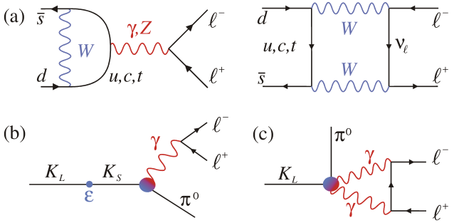
Figure 1: (a) Short-distance penguin and box diagrams for the initial conditions of $y_{7A,7V}$ in the SM. (b) $K^{0}-\bar{K}^{0}$ mixing-induced contribution, with a long-distance dominated, CP-conserving effective $K_{S}\rightarrow\pi^{0}\gamma^{\ast}$ vertex. (c) Long-distance two-photon induced CP-conserving contributions.

The indirect CP-violating contribution

(ICPV, Fig.1b) originates from $K^{0}-\bar{K}^{0}$ mixing. The subsequent CP-conserving $K_{S}\rightarrow\pi^{0}\ell^{+}\ell^{-}$ decay is dominated by the long-distance process $K_{S}\rightarrow\pi^{0}\left(\gamma^{\ast}\rightarrow\ell^{+}\ell^{-}\right)$, producing the lepton pair in a $1^{--}$ state. The corresponding amplitude reads:

$$\mathcal{M}_{\mathrm{ICPV}}=\varepsilon\,\mathcal{M}\left(K_{1}\rightarrow\pi^{0}\ell^{+}\ell^{-}\right)=-\varepsilon\frac{G_{F}\alpha_{em}}{4\pi}W_{S}\left(z\right)\left(P+K\right)^{\mu}\left\{\bar{u}_{p}\gamma_{\mu}v_{p^{\prime}}\right\}\;,$$ (2)

where $P,K,p$ and $p^{\prime}$ denote the momenta of the $K,\pi,\ell^{-}$ and $\ell^{+}$ states, respectively, $z=T^{2}/M_{K^{0}}^{2}$ with $T=p+p^{\prime}$ and $\alpha_{em}\approx 1/137$. The $W_{S}$ function has been analyzed in detail in Chiral Perturbation Theory (ChPT) in Ref.[1], and can be parametrized as follows:

$$W_{S}\left(z\right)=a_{S}+b_{S}z+W_{S}^{\pi\pi}\left(z\right)+W_{S}^{KK}\left(z\right)\;.$$ (3)

The pion and kaon loops ($W_{S}^{\pi\pi},W_{S}^{KK}$) were found small and, to a good approximation, a single (real) counterterm dominates: $W_{S}\left(z\right)\approx a_{S}$. This counterterm can then be extracted from the experimental $K_{S}\rightarrow\pi^{0}e^{+}e^{-}$ and $K_{S}\rightarrow\pi^{0}\mu^{+}\mu^{-}$ branching fractions: $\left|a_{S}\right|=1.20\pm 0.20$ [18]. Eq.(2) is thus indeed entirely determined in terms of measured quantities ($|a_{S}|$, $\varepsilon$).

The two-photon CP-conserving contribution

(Fig.1c), $K_{L}\rightarrow\pi^{0}\left(\gamma^{\ast}\gamma^{\ast}\rightarrow\ell^{+}\ell^{-}\right)$, produces the lepton pair in either a phase-space suppressed tensor state $2^{++}$ or a helicity-suppressed scalar state $0^{++}$. The former is found negligible from experimental constraints on $K_{L}\rightarrow\pi^{0}\left(\gamma\gamma\right)_{2^{++}}$[2], while for the latter the amplitude reads:

$$\mathcal{M}_{\mathrm{\gamma\gamma}}=\frac{G_{8}\alpha_{em}^{2}}{2\pi^{2}}M_{K}\frac{r_{\ell}}{z}\mathcal{F}_{\ell}\left(z\right)\left\{\bar{u}_{p}v_{p^{\prime}}\right\}\;,$$ (4)

with $r_{\ell}=m_{\ell}/M_{K}$ and $\left|G_{8}\right|=9.1\cdot 10^{-12}$ MeV^-2. It is dominated by the two-loop process $K_{L}\rightarrow\pi^{0}\left(P^{+}P^{-}\rightarrow\gamma^{\ast}\gamma^{\ast}\rightarrow\ell^{+}\ell^{-}\right)_{0^{++}}$ with $P=\pi,K$, computed in ChPT, and closely related to $K_{S}\rightarrow\pi^{+}\pi^{-}\rightarrow\gamma^{\ast}\gamma^{\ast}\rightarrow\ell^{+}\ell^{-}$. With the parametrization $\mathcal{M}\left(K_{L}\rightarrow\pi^{0}P^{+}P^{-}\right)\sim a_{1}^{P}\left(z\right)$ for the momentum distribution entering the subprocess $P^{+}P^{-}\rightarrow\gamma^{\ast}\gamma^{\ast}\rightarrow\ell^{+}\ell^{-}$, the two-loop form-factor $\mathcal{F}_{\ell}\left(z\right)$ can be expressed as ($r_{\pi}=M_{\pi}/M_{K}$)

$$\mathcal{F}_{\ell}\left(z\right)=a_{1}^{\pi}\left(z\right)\mathcal{I}\left(\frac{r_{\ell}^{2}}{z},\frac{r_{\pi}^{2}}{z}\right)-a_{1}^{K}\left(z\right)\mathcal{I}\left(\frac{r_{\ell}^{2}}{z},\frac{1}{z}\right)\;,$$ (5)

with $\mathcal{I}\left(a,b\right)$ given in Refs.[19, 3] (for practical purposes, a numerical representation is given in Appendix B).

A reliable estimation of $\Gamma\left(K_{L}\rightarrow\pi^{0}\ell^{+}\ell^{-}\right)_{\mathrm{\gamma\gamma}}$ can then be obtained from the measured $K_{L}\rightarrow\pi^{0}\gamma\gamma$ rate[20] thanks to the stability of the ratio

$$R_{\mathrm{\gamma\gamma}}=\frac{\Gamma\left(K_{L}\rightarrow\pi^{0}\ell^{+}\ell^{-}\right)_{\mathrm{\gamma\gamma}}}{\Gamma\left(K_{L}\rightarrow\pi^{0}\gamma\gamma\right)}\;,$$ (6)

with respect to changes in $a_{1}^{P}\left(z\right)$ [3]. Note that some $\mathcal{O}\left(p^{6}\right)$ ChPT effects are thus included in the estimated $\Gamma\left(K_{L}\rightarrow\pi^{0}\ell^{+}\ell^{-}\right)_{\mathrm{\gamma\gamma}}$, most notably those responsible for the large observed $K_{L}\rightarrow\pi^{0}\gamma\gamma$ rate compared to the $\mathcal{O}\left(p^{4}\right)$ ChPT prediction.

However, theoretical control over $R_{\mathrm{\gamma\gamma}}$ only is not sufficient to deal with New Physics interactions that produce the lepton pair in a $0^{++}$ state (generating interference effects) or compute forward-backward asymmetries. For this, we need to control $\mathcal{M}_{\mathrm{\gamma\gamma}}$ too. To fill this gap, the key is to use the similarity of behavior of the $K_{L}\rightarrow\pi^{0}\gamma\gamma$ and $K_{L}\rightarrow\pi^{0}\ell^{+}\ell^{-}$ spectra at the origin of the stability of $R_{\mathrm{\gamma\gamma}}$. First consider the fact that the $K_{L}\rightarrow\pi^{0}\gamma\gamma$ normalized spectrum is rather well-described with the parametrizations

$$\mathcal{O}\left(p^{4}\right)\;\text{ChPT} :a_{1}^{\pi}\left(z\right)_{ChPT}=z-r_{\pi}^{2},$$ (7a)

$$K_{L}\overset{}{\rightarrow}\pi^{0}\pi^{+}\pi^{-}\text{ Dalitz} :a_{1}^{\pi}\left(z\right)_{Dalitz}=-0.46+2.44z-0.95z^{2}\,,$$ (7b)

and $$a_{1}^{K}\left(z\right)=z-1-r_{\pi}^{2} a_{1}^{\pi}\left(z\right)_{Dalitz} z K_{L}\rightarrow\pi^{0}\pi^{+}\pi^{-} \mathcal{B}\left(K_{L}\rightarrow\pi^{0}\ell^{+}\ell^{-}\right)_{\mathrm{\gamma\gamma}} \mathcal{B}\left(K_{L}\rightarrow\pi^{0}\gamma\gamma\right)^{\exp} a_{1}^{P}\left(z\right)_{ChPT}\rightarrow 1.45a_{1}^{P}\left(z\right)_{ChPT} a_{1}^{P}\left(z\right)_{Dalitz}\rightarrow 1.36a_{1}^{P}\left(z\right)_{Dalitz} K_{L}\rightarrow\pi^{0}\ell^{+}\ell^{-} a_{1}^{\pi}\left(z\right)_{ChPT} a_{1}^{\pi}\left(z\right)_{Dalitz}$$ in both cases. For , only the -dependent part of the effective vertex is kept. Now, to account for the rescaling of by , we rescale and , such that the rate computed from Eq.(4) is kept frozen. Clearly, the theoretical control on the resulting differential rate is not as good as on the total rate, but is nevertheless satisfactory. In practice, the error inherent to the procedure can be probed by comparing the predictions obtained using either or .

Finally, as far as the sign of $\mathcal{M}_{\mathrm{\gamma\gamma}}$ is concerned, we checked that Eq.(4) is consistent with the conventions used in the rest of the paper for hadronic matrix elements. Furthermore, under the reasonable assumption that the sign of $G_{8}$ as fixed by the factorization approximation is not changed by the non-perturbative evolution down to $M_{K}$ (see for example Ref.[21]), our conventions correspond to $G_{8}<0$.

2.2 Vector and axial-vector short-distance contributions

Let us now consider the DCPV piece induced by the vector and axial-vector operators of Eq.(1):

$$\mathcal{M}_{\mathrm{V,A}}=\langle\pi^{0}\ell^{+}\ell^{-}|-\mathcal{H}_{eff}^{\mathrm{V,A}}|K_{L}\rangle=iG_{F}\alpha\langle\pi^{0}|\bar{s}\gamma_{\mu}d|K^{0}\rangle\left\{\bar{u}_{p}\gamma^{\mu}\left(\operatorname{Im}\left(\lambda_{t}y_{7V}\right)+\operatorname{Im}\left(\lambda_{t}y_{7A}\right)\gamma_{5}\right)v_{p^{\prime}}\right\}$$ (8)

(the sizeable $c$-quark contribution, known at NLO[13], is understood in $y_{7V}$), with the matrix element

$$\langle\pi^{0}\left(K\right)|\bar{s}\gamma^{\mu}d|K^{0}\left(P\right)\rangle=\frac{1}{\sqrt{2}}\left(\left(P+K\right)^{\mu}f_{+}^{K^{0}\pi^{0}}\left(z\right)+\left(P-K\right)^{\mu}f_{-}^{K^{0}\pi^{0}}\left(z\right)\right)\;,$$ (9)

$$f_{-}^{K^{0}\pi^{0}}\left(z\right)=\frac{1-r_{\pi}^{2}}{z}\left(f_{0}^{K^{0}\pi^{0}}\left(z\right)-f_{+}^{K^{0}\pi^{0}}\left(z\right)\right)\;.$$

The slopes are extracted from $K_{\ell 3}$ decays [23, 22], neglecting isospin breaking:

$$f_{0,+}\left(z\right)\equiv f_{0,+}^{K^{0}\pi^{0}}\left(z\right)=\frac{f_{+}\left(0\right)}{1-\lambda_{0,+}z},\;\;\lambda_{0}=0.18\text{, }\lambda_{+}=0.32\;,$$ (10)

in the pole parametrization. Accounting for isospin breaking in $\pi^{0}-\eta$ mixing for the value at zero momentum transfer[24], one gets:

$$f_{+}\left(0\right)=\left(1.0231\right)^{-1}f_{+}^{K^{0}\pi^{+}}\left(0\right)\approx 0.939\;,$$ (11)

with the Leutwyler-Ross prediction $f_{+}^{K^{0}\pi^{+}}\left(0\right)=0.961\left(8\right)$[25], confirmed by lattice studies[26]. This quite precise value, together with the knowledge of the form-factor slopes, renders the theoretical prediction of the vector and axial-vector contributions to $K_{L}\rightarrow\pi^{0}\ell^{+}\ell^{-}$ remarkably clean.

Inserting Eq.(9) in $\mathcal{M}_{\mathrm{V,A}}$, the vector current is seen to produce the lepton pair in a vector state $1^{--}$, while the axial-vector part produces it in an axial-vector $1^{++}$ or pseudoscalar $0^{-+}$ state. This latter component is helicity suppressed, and enters thus only the muon mode. Besides, the vector current and ICPV amplitudes produce the same final state, they thus interfere in the rate. Recent theoretical analyses point towards a constructive interference, i.e., $a_{S}<0$ [2, 27].

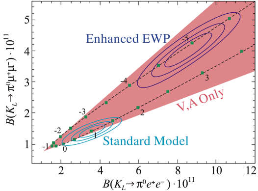
Figure 2: Behavior of $\mathcal{B}\left(K_{L}\rightarrow\pi^{0}\mu^{+}\mu^{-}\right)$ against $\mathcal{B}\left(K_{L}\rightarrow\pi^{0}e^{+}e^{-}\right)$, in units of $10^{-11}$, as $y_{7A,7V}$ are rescaled by a common factor (dots), or allowed to take arbitrary values (red sector). The ellipses denote $25,50,75\%$ confidence regions in the SM, assuming constructive DCPV – ICPV interference (destructive interference is around the $-1$ dot), or for Ref.[17], in which $y_{7A}\approx-3.2$ and $y_{7V}\approx 0.9$.

Total rates:

Altogether, the branching ratios are predicted to be

$$\mathcal{B}_{\mathrm{V,A}}^{\ell^{+}\ell^{-}}=\left(C_{dir}^{\ell}\pm C_{int}^{\ell}\left|a_{S}\right|+C_{mix}^{\ell}\left|a_{S}\right|^{2}+C_{\gamma\gamma}^{\ell}\right)\cdot 10^{-12}\;,\vskip 3.0pt plus 1.0pt minus 1.0pt$$ (12)

$$C_{dir}^{e}=\left(4.62\pm 0.24\right)\;\left(w_{7V}^{2}+w_{7A}^{2}\right),$$

(17)

with $w_{7A,7V}=\operatorname{Im}\left(\lambda_{t}y_{7A,7V}\right)/\operatorname{Im}\lambda_{t}$. In the Standard Model, the coefficients $y_{7A,7V}$ are real [13]:

$$y_{7A}\left(M_{W}\right)=-0.68\pm 0.03,\;\;y_{7V}\left(\mu\approx 1\;\text{GeV}\right)=0.73\pm 0.04\;,$$ (18)

and, with $\operatorname{Im}\lambda_{t}=\left(1.407\pm 0.098\right)\cdot 10^{-4}$[28], one gets

$$\mathcal{B}_{\mathrm{SM}}^{e^{+}e^{-}}=3.54_{-0.85}^{+0.98}\;\left(1.56_{-0.49}^{+0.62}\right)\cdot 10^{-11},\;\;\mathcal{B}_{\mathrm{SM}}^{\mu^{+}\mu^{-}}=1.41_{-0.26}^{+0.28}\;\left(0.95_{-0.21}^{+0.22}\right)\cdot 10^{-11}\;,$$ (19)

for constructive (destructive) interference. The present experimental bounds are one order of magnitude above these predictions:

$$\mathcal{B}_{\mathrm{\exp}}^{e^{+}e^{-}}<28\cdot 10^{-11}\text{\cite[cite]{[\@@bibref{}{KTeVelec}{}{}]}},\;\;\mathcal{B}_{\mathrm{\exp}}^{\mu^{+}\mu^{-}}<38\cdot 10^{-11}\text{\cite[cite]{[\@@bibref{}{KTeVmuon}{}{}]}}\;.$$ (20)

The differential rate for the electronic mode is trivial (no CPC piece), while for the muonic mode it can be found in Ref.[3].

The Standard Model confidence region on the $\mathcal{B}^{e^{+}e^{-}}$–$\mathcal{B}^{\mu^{+}\mu^{-}}$ plane is shown in Fig.2. As discussed in Ref.[3], this plane is particularly well-suited to search for New Physics signal, and identify its specific nature. Indeed, the fact that helicity suppression is rather inefficient for the muonic mode introduces a genuine difference of sensitivity to the short-distance V,A currents, i.e. to $y_{7A,7V}$, for the two $K_{L}\rightarrow\pi^{0}\ell^{+}\ell^{-}$ modes. These two types of contributions can thus be disentangled by measuring both rates. Suffices to note that the coefficients approximately obey $C_{i}^{\mu}/C_{i}^{e}\approx 0.23$, $i=dir,int,mix$, which is simply the phase-space suppression, except for the enhanced $y_{7A}$ contribution to $C_{dir}^{\mu}$, which comes from the production of helicity-suppressed pseudoscalar $0^{-+}$ states. Without this, no matter the New Physics contributions to $y_{7A,7V}$, the rates would always fall on a trivial straight line. Thanks to this effect, on the contrary, for arbitrary values of $y_{7A,7V}$, the two modes can lie anywhere inside the red sector in Fig.2 for the $C_{i}^{\ell}$ at their central values. Accounting for theoretical errors at $1\sigma$, this area is mathematically expressed as

$$0.1\cdot 10^{-11}+0.24\mathcal{B}_{\mathrm{V,A}}^{e^{+}e^{-}}<\mathcal{B}_{\mathrm{V,A}}^{\mu^{+}\mu^{-}}<0.6\cdot 10^{-11}+0.58\mathcal{B}_{\mathrm{V,A}}^{e^{+}e^{-}}\;.$$ (21)

For definiteness, we have also indicated the curve corresponding to a common rescaling of $y_{7A}$ and $y_{7V}$ from New Physics, and drawn the confidence region for the enhanced electroweak penguins of Ref.[17], to illustrate the opposite situation in which $y_{7A}=-3.2$ is strongly enhanced, while $y_{7V}=0.9$ stays roughly the same as in the SM. Finally, note that the extent of the confidence regions essentially reflects the uncertainty on $a_{S}$ (whose effect is included in the bounds Eq.(21)), and could be reduced by more precise measurements of the $K_{S}\rightarrow\pi^{0}\ell^{+}\ell^{-}$ branching fractions.

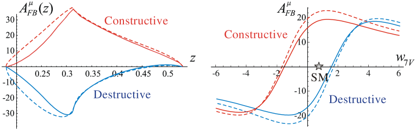
Figure 3: Left: $A_{FB}^{\mu}$ (in %) as a function of $z$, in the SM. Right: Integrated $A_{FB}^{\mu}$ (in %) as a function of $w_{7V}$, with $w_{7A}$ fixed at its SM value. Red (blue) lines correspond to constructive (destructive) interference between ICPV and vector current contributions, while plain (dashed) lines correspond to $a_{1}^{P}\left(z\right)_{Dalitz}$ ($a_{1}^{P}\left(z\right)_{ChPT}$), respectively.

Forward-backward asymmetry:

The differential forward-backward asymmetry[11, 12] is defined by

$$A_{FB}^{\ell}\left(z\right)=\frac{{\displaystyle\int_{0}^{y_{0}}}\dfrac{d^{2}\Gamma}{dydz}dy-{\displaystyle\int_{-y_{0}}^{0}}\dfrac{d^{2}\Gamma}{dydz}dy}{{\displaystyle\int_{0}^{y_{0}}}\dfrac{d^{2}\Gamma}{dydz}dy+{\displaystyle\int_{-y_{0}}^{0}}\dfrac{d^{2}\Gamma}{dydz}dy}\;,$$ (22)

with

$$y=\frac{P\cdot(p-p^{\prime})}{M_{K}^{2}},\;\;y_{0}=\frac{1}{2}\beta_{\ell}\beta_{\pi}\;,$$ (23)

and $\beta_{\ell}^{2}=1-4r_{\ell}^{2}/z$, $\beta_{\pi}^{2}=\lambda\left(1,r_{\pi}^{2},z\right)$, $\lambda\left(a,b,c\right)=a^{2}+b^{2}+c^{2}-2\left(ab+bc+ac\right).$ The variable $y$ is related to the angle between the $K$ and $\ell^{-}$ momenta in the dilepton rest-frame (hence the name forward-backward), and also, by definition, to the energy difference $E_{\ell^{-}}-E_{\ell^{+}}$ in the $K$ rest-frame (one then speaks of lepton energy asymmetry).

This observable requires CP-violation, and arises from the $\operatorname{Re}[\mathcal{M}_{\mathrm{1}^{--}}^{\ast}\left(\mathcal{M}_{\mathrm{0}^{++}}+\mathcal{M}_{\mathrm{2}^{++}}\right)]$ interference term. Let us start by assuming that $\mathcal{M}_{\mathrm{2}^{++}}$ is negligible, as for the total rates. Then:

$$A_{FB}^{\ell}\left(z\right)=\frac{A_{1}^{\ell}\left(z\right)}{d\Gamma/dz}\operatorname{Re}\left(\varepsilon^{\ast}W_{S}^{\ast}\left(z\right)\mathcal{F}_{\ell}\left(z\right)\right)+\frac{A_{2}^{\ell}\left(z\right)}{d\Gamma/dz}\operatorname{Im}\left(\lambda_{t}y_{7V}\right)\operatorname{Im}\mathcal{F}_{\ell}\left(z\right)\;,$$ (24)

with $A_{1,2}^{\ell}\left(z\right)$ some combinations of constants and form-factors. The electronic asymmetry $A_{FB}^{e}\left(z\right)$ is negligible in this case since $\mathcal{F}_{e}\left(z\right)$ is helicity suppressed, while for the muon it is shown in Fig.3 in the case of the Standard Model. Note that the theoretical control gained over this quantity would be difficult to improve since it relies on the specific parametrization of $\mathcal{M}_{\mathrm{\gamma\gamma}}$. In addition, the experimental sensitivity required to measure $A_{FB}^{\ell}\left(z\right)$ is unlikely to be achieved soon. We will therefore not consider $A_{FB}^{\ell}\left(z\right)$ anymore, but rather concentrate on the integrated asymmetry:

$$A_{FB}^{\ell}=\frac{{\displaystyle\int_{4r_{\ell}^{2}}^{(1-r_{\pi})^{2}}}dz\left({\displaystyle\int_{0}^{y_{0}}}\dfrac{d^{2}\Gamma}{dydz}dy-{\displaystyle\int_{-y_{0}}^{0}}\dfrac{d^{2}\Gamma}{dydz}dy\right)}{{\displaystyle\int_{4r_{\ell}^{2}}^{(1-r_{\pi})^{2}}}dz\left({\displaystyle\int_{0}^{y_{0}}}\dfrac{d^{2}\Gamma}{dydz}dy+{\displaystyle\int_{-y_{0}}^{0}}\dfrac{d^{2}\Gamma}{dydz}dy\right)}=\frac{N\left(E_{\ell^{-}}>E_{\ell^{+}}\right)-N\left(E_{\ell^{-}}<E_{\ell^{+}}\right)}{N\left(E_{\ell^{-}}>E_{\ell^{+}}\right)+N\left(E_{\ell^{-}}<E_{\ell^{+}}\right)}\;.$$ (25)

Compared to $A_{FB}^{\mu}\left(z\right)$, it is more stable:

$$A_{FB}^{\mu}=\left(1.3\left(1\right)w_{7V}\pm 1.7(2)\left|a_{S}\right|\right)\cdot 10^{-12}\,\text{\thinspace}/\,\mathcal{B}_{\mathrm{V,A}}^{\mu^{+}\mu^{-}}\;.$$ (26)

In the Standard Model, $A_{FB}^{\mu}=\left(20\pm 4\right)\%$ for constructive and $\left(-12\pm 4\right)\%$ for destructive interference, with the error coming from varying $a_{1}^{\pi}\left(z\right)$ between $\mathcal{O}\left(p^{4}\right)$ ChPT and Dalitz accounting for $\pm 2\%$.

For general axial currents, it is clear that $A_{FB}^{\mu}$ decreases when $w_{7A}$ increases since it does not contribute to the interference Eq.(24). For $w_{7V}$, the interference is linear while the rate is quadratic, and thus $|A_{FB}^{\mu}|$ reaches a maximum, around $23\%$ for $w_{7A}$ at its SM value, before decreasing again, see Fig.3. The absolute maximum for $A_{FB}^{\mu}$ is around $\pm 25\%$ for $w_{7A}\approx 0$ and $w_{7V}\approx\pm 1$ or $\pm 4$, depending on the direct - indirect CPV interference sign.

In the SM, even if $A_{FB}^{\mu}$ is polluted by the theoretical error on the two-photon amplitude, its measurement could fix the sign of $a_{S}$. As can be seen in Fig.3, this remains true if New Physics is found from the measurements of $K_{L}\rightarrow\pi^{0}\ell^{+}\ell^{-}$ total rates with $|w_{7V}|\lesssim 2$.

Let us now consider the interference term $\operatorname{Re}[\mathcal{M}_{\mathrm{1}^{--}}^{\ast}\mathcal{M}_{\mathrm{2}^{++}}]$. The amplitude $\mathcal{M}_{\mathrm{2}^{++}}$ is discussed in detail in Ref.[2]. It leads to a helicity-allowed, but phase-space suppressed contribution to $A_{FB}^{\ell}$, hence contributes mostly for the electronic mode. Unfortunately, the theoretical control on the $\mathcal{M}_{\mathrm{2}^{++}}$ amplitude is not good as it depends on unknown phenomenological parameters. Though sufficient for deriving, from $K_{L}\rightarrow\pi^{0}\gamma\gamma$, a tight upper bound on the $\mathrm{2}^{++}$ contribution to $C_{\gamma\gamma}^{\ell}$ in Eq.(12)[2], $A_{FB}^{e}$ remains largely unconstrained. Indeed, both $\mathcal{M}_{\mathrm{1}^{--}}^{\ast}$ and $\mathcal{M}_{\mathrm{2}^{++}}$ contribute mostly at low $z$, and their sizeable interference can generate $A_{FB}^{e}$ anywhere between $0\%$ and about $\pm 60\%$[11], depending on the phenomenological parameters of Ref.[2].

Concerning $A_{FB}^{\mu}$, the situation is better. The impact of $\mathcal{M}_{\mathrm{2}^{++}}$ corresponds to an additional $\pm 3\%$ uncertainty, and therefore does not affect the potential of $A_{FB}^{\mu}$ in determining the sign of $a_{S}$.

3 $K_{L}\rightarrow\pi^{0}\ell^{+}\ell^{-}$ with generic new physics operators

In addition to the modification of vector and axial-vector couplings considered in the previous section, new four-fermion effective interactions could be generated by the integration of New Physics heavy degrees of freedom. The effective Hamiltonian comprising all the possible dimension-six semi-leptonic four-fermion structures[31] relevant for $K_{L}\rightarrow\pi^{0}\ell^{+}\ell^{-}$ (as well as quark bilinear electromagnetic couplings) reads

$$\mathcal{H}_{eff}=\mathcal{H}_{eff}^{\mathrm{V,A}}+\mathcal{H}_{eff}^{\mathrm{P,S}}+\mathcal{H}_{eff}^{\mathrm{T,\tilde{T}}}+\mathcal{H}_{eff}^{\mathrm{EMO}}\;,$$ (27)

with $\mathcal{H}_{eff}^{\mathrm{V,A}}$ given in Eq.(1) and

$$\mathcal{H}_{eff}^{\mathrm{P,S}} =\frac{G_{F}^{2}M_{W}^{2}}{\pi^{2}}\frac{m_{s}m_{\ell}}{M_{W}^{2}}\left[y_{P}\left(\bar{s}d\right)\left(\bar{\ell}\gamma_{5}\ell\right)+y_{S}\left(\bar{s}d\right)\left(\bar{\ell}\ell\right)\right]+h.c.$$ (28)

$$\mathcal{H}_{eff}^{\mathrm{T,\tilde{T}}} =\frac{G_{F}^{2}M_{W}^{2}}{\pi^{2}}\frac{m_{s}m_{\ell}}{M_{W}^{2}}\left[y_{T}\left(\bar{s}\sigma_{\mu\nu}d\right)\left(\bar{\ell}\sigma^{\mu\nu}\ell\right)+y_{\tilde{T}}\left(\bar{s}\sigma_{\mu\nu}d\right)\left(\bar{\ell}\sigma^{\mu\nu}\gamma_{5}\ell\right)\right]+h.c.$$ (29)

$$\mathcal{H}_{eff}^{\mathrm{EMO}} =\frac{G_{F}}{\sqrt{2}}M_{K}\frac{Q_{d}e}{16\pi^{2}}\left[y_{\gamma}^{\pm}\left(\bar{s}\sigma_{\mu\nu}\left(1\pm\gamma_{5}\right)d\right)F^{\mu\nu}\right]+h.c.\;\;.$$ (30)

A low scale ($\mu\lesssim m_{c}$) is understood for the evaluation of the Wilson coefficients, quark masses and matrix elements of the operators in the above equation. Dimension-eight operators, containing two powers of the external momenta, are not considered as they are very small in the SM and are expected to remain so in the presence of New Physics (see discussion in [32]).

Our goal is to analyze the impact of these new operators on the $K_{L}\rightarrow\pi^{0}\ell^{+}\ell^{-}$ branching fractions and asymmetries in a model-independent way. Still, some comments on specific scenarios behind the various operators are in order:

1. For the scalar and pseudoscalar operators $Q_{S}=\left(\bar{s}d\right)\left(\bar{\ell}\ell\right)$ and $Q_{P}=\left(\bar{s}d\right)\left(\bar{\ell}\gamma_{5}\ell\right)$, we have explicitly included the $m_{s}m_{\ell}/M_{W}^{2}$ helicity suppression factor to give a realistic description of models where these operators are generated from an extended Higgs sector. For example, large $y_{P,S}$ can arise in the MSSM with large $\tan\beta$ (see e.g. [5, 6]) and sizeable trilinear soft-breaking couplings. This kind of scenarios has been analyzed in many works, but usually focuses on other decay modes. See e.g. Refs.[33, 32] for a MSSM analysis with emphasis on the $K,B\rightarrow\ell^{+}\ell^{-}$ decays.

2. The tensor and pseudotensor operators $Q_{T}=\left(\bar{s}\sigma_{\mu\nu}d\right)\left(\bar{\ell}\sigma^{\mu\nu}\ell\right)$ and $Q_{\tilde{T}}=\left(\bar{s}\sigma_{\mu\nu}d\right)\left(\bar{\ell}\sigma^{\mu\nu}\gamma_{5}\ell\right)=i\varepsilon^{\mu\nu\rho\sigma}\left(\bar{s}\sigma_{\mu\nu}d\right)\left(\bar{\ell}\sigma_{\rho\sigma}\gamma_{5}\ell\right)$, to our knowledge, have not been included in studies of $K_{L}\rightarrow\pi^{0}\ell^{+}\ell^{-}$ so far. These modes are however the most promising source of information on $Q_{T,\tilde{T}}$, since these cannot contribute to $K\rightarrow\ell^{+}\ell^{-}$. Though they do not arise in the SM, they do in the MSSM but, in addition to being helicity suppressed, they are usually suppressed by loop factors[32]. Similar operators have been considered in $\Delta F=2$ processes (see e.g. Refs.[34, 35]) and for the $B\rightarrow X\ell^{+}\ell^{-}$ rate and asymmetries (see e.g. Ref.[36]).

3. For completeness, we have included the dimension-five electromagnetic tensor operators $Q_{\gamma}^{\pm}=\left(\bar{s}\sigma_{\mu\nu}\left(1\pm\gamma_{5}\right)d\right)F^{\mu\nu}$. These were considered for example in Refs.[9, 10]. Since the $\sigma_{\mu\nu}\gamma_{5}$ part does not contribute to $K_{L}\rightarrow\pi^{0}\ell^{+}\ell^{-}$, only $y_{\gamma}\equiv y_{\gamma}^{+}+y_{\gamma}^{-}$ is accessible here. Note that in principle these operators already arise in the Standard Model, however they are too small to affect $K_{L}\rightarrow\pi^{0}\ell^{+}\ell^{-}$. In the MSSM, they are correlated with the chromomagnetic tensor operators and thus strongly constrained by other observables[9, 10].

4. In the last section, we consider the general framework in which neither $Q_{S,P}$ nor $Q_{T,\tilde{T}}$ are helicity-suppressed, i.e. we remove the $m_{s}m_{\ell}/M_{W}^{2}$ factors in Eqs.(28,29). A large class of models with such helicity-allowed FCNC operators are theories with leptoquark interactions (for a review, see [8]), among which specific GUT models. Alternatively, SUSY without R-parity can also induce helicity-allowed $Q_{S,P}$ interactions through tree-level sneutrino exchanges (see e.g. [7]).

The distinction between helicity-suppressed and helicity-allowed scenarios is necessary as the corresponding signatures, i.e. impacts on $K_{L}\rightarrow\pi^{0}e^{+}e^{-}$ and $K_{L}\rightarrow\pi^{0}\mu^{+}\mu^{-}$, will obviously be very different. Let us now analyze these impacts systematically.

3.1 Scalar and pseudoscalar operators

The relevant matrix element reads

$$\langle\pi^{0}|\bar{s}d|K^{0}\rangle=-\frac{M_{K}^{2}-M_{\pi}^{2}}{\sqrt{2}\left(m_{s}-m_{d}\right)}f_{0}\left(z\right)\;$$ (31)

in the sign convention of Eq.(9). This matrix element is enhanced compared to its vector counterpart due to the large value of the quark condensate (i.e., the large ratio of meson masses over quark masses).

The scalar (pseudoscalar) operator produces the lepton pair in a CP-even $0^{++}$ (CP-odd $0^{-+}$) state, therefore it is the real (imaginary) part of its Wilson coefficient that contributes to $K_{L}\rightarrow\pi^{0}\ell^{+}\ell^{-}$:

$$\mathcal{M}_{\mathrm{P}} =\frac{G_{F}^{2}M_{W}^{2}}{\pi^{2}}\frac{m_{\ell}}{M_{W}^{2}}\left(M_{K}^{2}-M_{\pi}^{2}\right)\;i\operatorname{Im}y_{P}\;f_{0}\left(z\right)\;\left\{\bar{u}_{p}\gamma_{5}v_{p^{\prime}}\right\}\;,$$ (32)

$$\mathcal{M}_{\mathrm{S}} =\frac{G_{F}^{2}M_{W}^{2}}{\pi^{2}}\frac{m_{\ell}}{M_{W}^{2}}\left(M_{K}^{2}-M_{\pi}^{2}\right)\;\operatorname{Re}y_{S}\;f_{0}\left(z\right)\;\left\{\bar{u}_{p}v_{p^{\prime}}\right\}\;.$$ (33)

To reach these expressions, $m_{d}$ has been neglected against $m_{s}$ in Eq.(31). The pseudoscalar current interferes with the helicity-suppressed pseudoscalar part of the axial-vector current, while the scalar current interferes with the helicity-suppressed two–photon 0⁺⁺ contribution. Since in addition $Q_{S}$ and $Q_{P}$ are themselves helicity-suppressed, only the muon mode can be affected by $y_{S,P}$.

For the pseudoscalar operator,

including also the $\mathrm{V}$ and $\mathrm{A}$ contributions, the differential rate reads:

$$\frac{d\Gamma_{\mathrm{V,A\&P}}}{dz}=\frac{G_{F}^{2}M_{K}^{5}\alpha^{2}}{64\pi^{3}}\left(\operatorname{Im}\lambda_{t}\right)^{2}\beta_{\ell}\beta_{\pi}\left(\frac{\beta_{\pi}^{2}}{6}A_{+}\left(f_{+}\left(z\right)\right)^{2}+A_{0}\left(f_{0}\left(z\right)\right)^{2}\right),$$ (34)

$$A_{+}=w_{7A}^{2}\beta_{\ell}^{2}+w_{7V}^{2}\frac{3-\beta_{\ell}^{2}}{2},\;\;A_{0}=\frac{r_{\ell}^{2}}{z}\left(w_{7A}\left(1-r_{\pi}^{2}\right)+z\rho_{P}\operatorname{Im}y_{P}\right)^{2},$$

with the prefactor

$$\rho_{P}=\frac{1}{\operatorname{Im}\lambda_{t}}\frac{1}{2\pi\sin^{2}\theta_{W}}\frac{M_{K}^{2}-M_{\pi}^{2}}{M_{W}^{2}}\approx 0.18\;.$$ (35)

$\operatorname{Im}y_{P}\sim\mathcal{O}\left(10\right)$ is thus required to get $\mathcal{O}\left(1\right)$ effects. Numerically, the contributions to the total rates, to be added to Eq.(12), are

$$\mathcal{B}_{\mathrm{P}}^{e^{+}e^{-}} =\left(1.9\,w_{7A}\,\operatorname{Im}y_{P}+0.038\left(\operatorname{Im}y_{P}\right)^{2}\right)\cdot 10^{-17}\;,$$ (36a)

$$\mathcal{B}_{\mathrm{P}}^{\mu^{+}\mu^{-}} =\left(0.26\,w_{7A}\,\operatorname{Im}y_{P}+0.0085\left(\operatorname{Im}y_{P}\right)^{2}\right)\cdot 10^{-12}\;,$$ (36b)

showing the very strong helicity suppression at play for the electron mode.

For the scalar operator,

from Eqs.(4) and (33), one immediately gets for the total $0^{++}$ contribution:

$$\frac{d\Gamma_{\mathrm{\gamma\gamma\&S}}}{dz}=\frac{G_{8}^{2}M_{K}^{5}\alpha_{em}^{4}}{512\pi^{7}}\beta_{\pi}\beta_{\ell}^{3}\frac{r_{\ell}^{2}}{z}\left|\mathcal{F}_{\ell}\left(z\right)-\rho_{S}\operatorname{Re}y_{S}\,z\,f_{0}\left(z\right)\right|^{2}\;,$$ (37)

with the suppression factor

$$\rho_{S}=-\frac{\sqrt{2}\pi}{\sin^{2}\theta_{W}}\frac{\alpha G_{F}}{\alpha_{em}^{2}G_{8}}\frac{M_{K}^{2}-M_{\pi}^{2}}{M_{W}^{2}}\approx 0.13\;.$$ (38)

Since $\mathcal{F}_{\mu}\left(z\right)\sim\mathcal{O}\left(1\right)$, the helicity suppression $M_{W}^{-2}$ turns out to be nearly compensated. Performing the $z$ integral, we find

$$\mathcal{B}_{\mathrm{S}}^{e^{+}e^{-}} =(1.5\left(3\right)\operatorname{Re}y_{S}+0.0039\left(\operatorname{Re}y_{S}\right)^{2})\cdot 10^{-16}\;,$$ (39a)

$$\mathcal{B}_{\mathrm{S}}^{\mu^{+}\mu^{-}} =(0.04\left(1\right)\operatorname{Re}y_{S}+0.0041\left(\operatorname{Re}y_{S}\right)^{2})\cdot 10^{-12}\;.$$ (39b)

The error on the interference term is estimated by varying the distribution $$a_{1}^{\pi}\left(z\right) \mathcal{O}\left(p^{4}\right) 0.034 0.053$$ between ChPT and Dalitz (giving respectively and for the muonic mode).

Total rates:

The $Q_{S}$ and $Q_{P}$ operators do not affect the electronic mode due to their strong helicity suppression. For the muonic mode, combining Eqs.(36,39) with Eq.(12) and fixing $w_{7A,7V}$ at their SM values Eq.(18), the impacts on the total rate are summarized in the first three columns of Table 1.

Enhancement Enhancement Maximal Bound from Experimental of 50% of 100% suppression $K_{L}\rightarrow\mu^{+}\mu^{-}$ bound (Eq.(20)) $\operatorname{Im}y_{P}$ $-20,40$ $-30,50$ 7% for $\operatorname{Im}y_{P}\approx 10\;\,\,$ $\left|\operatorname{Im}y_{P}\right|\lesssim 8$ $|\operatorname{Im}y_{P}|\lesssim 220$ $\operatorname{Re}y_{S}$ $-45,35$ $-65,55$ 1% for $\operatorname{Re}y_{S}\approx-5$ $\left|\operatorname{Re}y_{S}\right|\lesssim 50$ $|\operatorname{Re}y_{S}|\lesssim 300$

Table 1: Numerical analysis of scalar and pseudoscalar operator impacts on $\mathcal{B}^{\mu^{+}\mu^{-}}$.

A well-motivated scenario in which $\operatorname{Re}y_{S}$ and $\operatorname{Im}y_{P}$ can be large is the MSSM for large values of $\tan\beta$[5, 6]. In that context, the contributions of $Q_{S,P}$ are related to those of $Q_{P}^{\prime}=\left(\bar{s}\gamma_{5}d\right)\left(\bar{\ell}\gamma_{5}\ell\right)$ and $Q_{S}^{\prime}=(\bar{s}\gamma_{5}d)(\bar{\ell}\ell)$: $y_{S,P}=y_{P,S}^{\prime}$, with $y_{P}^{\prime}$ and $y_{S}^{\prime}$ further correlated. The contributions of $Q_{P,S}^{\prime}$ to $K_{L}\rightarrow\mu^{+}\mu^{-}$ were analyzed for example in Ref.[33], with the result that values of a few tens for $y_{S,P}^{\prime}$ are compatible with $\Delta S=2$ and $B$-physics data.

Without restricting ourselves to the MSSM, we can investigate the constraints on $y_{S,P}$ derived from the experimental $K_{L}\rightarrow\mu^{+}\mu^{-}$ rate under the assumption that $y_{S,P}=y_{P,S}^{\prime}$ approximately holds. This analysis is presented in Appendix A, leading to $\left|\operatorname{Im}y_{S}^{\prime}\right|\lesssim 8$ and $\left|\operatorname{Re}y_{P}^{\prime}\right|\lesssim 35$ for $y_{7A}^{\prime}=y_{7A}=-0.68$ (for the $Q_{7A}^{\prime}=\left(\bar{s}\gamma_{\mu}\gamma_{5}d\right)\left(\bar{\ell}\gamma^{\mu}\gamma_{5}\ell\right)$ operator). Allowing for New Physics in the axial-vector current with the bound $\left|y_{7A}^{\prime}\right|\lesssim 3$ corresponds to $\left|\operatorname{Re}y_{P}^{\prime}\right|\lesssim 70$, a much larger range since these two contributions interfere in the rate.

Our numerical analysis can be summarized drawing the allowed regions on the $\mathcal{B}^{e^{+}e^{-}}$–$\mathcal{B}^{\mu^{+}\mu^{-}}$ plane (Fig.4). Compared to the region spanned for general values of $y_{7A,7V}$ (Fig.2), turning on $y_{S,P}$ basically extends the vertical spread since only the muon mode is affected, and this mostly in the upward direction (i.e., enhancements). This is illustrated in Fig.4 by the light-blue/dark-blue region, corresponding to $|\operatorname{Re}y_{S}|<90$ / $|\operatorname{Im}y_{P}|<35$, respectively. Imposing further the constraints from $K_{L}\rightarrow\mu^{+}\mu^{-}$ under the assumption $y_{7A,S,P}=y_{7A,P,S}^{\prime}$ gives the yellow region. Obviously, the sensitivity of $K_{L}\rightarrow\pi^{0}\mu^{+}\mu^{-}$ to $Q_{S,P}$ is quite good.

It should also be noted that $Q_{S,P}$ contribute mostly for large $z$. While, as explained in Ref.[3], introducing a cut off at $z\approx 4r_{\ell}^{2}$ can reduce the contribution of the two-photon amplitude with respect to the $Q_{7A,7V}$ ones, thereby reducing the theoretical error, such a procedure would also reduce the sensitivity to $\operatorname{Im}y_{P}$ and $\operatorname{Re}y_{S}$ significantly, and may thus not be desirable.

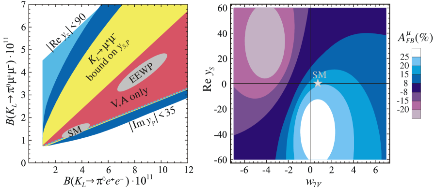
Figure 4: Left: Impacts of scalar and pseudoscalar operators in the $\mathcal{B}^{e^{+}e^{-}}-\mathcal{B}^{\mu^{+}\mu^{-}}$ plane of Fig.2. Light blue (dark blue) corresponds to arbitrary $y_{7A,7V}$ together with $\operatorname{Re}y_{S}<90$ ( $\operatorname{Im}y_{P}<35$), resp., while the yellow region corresponds to $y_{7V,7A,S,P}$ arbitrary but compatible with $\mathcal{B}\left(K_{L}\rightarrow\mu^{+}\mu^{-}\right)^{\exp}$ (see text). The dashed, light-blue line indicates the lower extent of the corresponding region. Right: The asymmetry $A_{FB}^{\mu}$ as a function of $w_{7V}$ and $\operatorname{Re}y_{S}$, assuming constructive interference ($a_{S}<0$), $y_{7A}=-0.68$ and $\operatorname{Im}y_{P}=0$.

Forward-backward asymmetry:

$\operatorname{Re}y_{S}$ enters the numerator of $A_{FB}^{\mu}$ through the interference term $\mathcal{M}_{\mathrm{ICPV}}^{\ast}\mathcal{M}_{\mathrm{S}}$ only:

$$A_{FB}^{\mu}=(1.3\left(1\right)w_{7V}\pm 1.7(2)\left|a_{S}\right|\mp 0.057\left|a_{S}\right|\operatorname{Re}y_{S})\cdot 10^{-12}\,\text{\thinspace}/\,\mathcal{B}_{\mathrm{V,A,S,P}}^{\mu^{+}\mu^{-}}\;.$$ (40)

There is no interference between $\mathcal{M}_{\mathrm{S}}$ and $\mathcal{M}_{\mathrm{V}}$ because of their 90^∘ relative phase. For this reason, $A_{FB}^{\mu}$ goes to zero when $y_{7V}$ and/or $\operatorname{Re}y_{S}$ becomes large, and reaches its maximum for moderate values, as shown in Fig.4 for $y_{7A}=-0.68$ and $\operatorname{Im}y_{P}=0$. If these latter two values are enhanced, since they contribute only to $\mathcal{B}_{\mathrm{V,A,S,P}}^{\mu^{+}\mu^{-}}$, $A_{FB}^{\mu}$ decreases, i.e. the figure remains the same but the absolute size of $A_{FB}^{\mu}$ is reduced. Finally, the figure for destructive interference is readily obtained by performing a vertical axis reflexion ($w_{7V}\rightarrow-w_{7V}$) followed by an overall sign change for $A_{FB}^{\mu}$.

No matter the New Physics behind $y_{7A,7V,S,P}$, $|A_{FB}^{\mu}|$ is always smaller than $30\%$, i.e., not very far from its SM value Eq.(26). Given the theoretical errors, $A_{FB}^{\mu}$ does not appear very promising to get a clear signal of New Physics. Nevertheless, as said before, it offers a very interesting possibility of constraining the relative signs of $\operatorname{Re}y_{S}$, $y_{7V}$ and $a_{S}$ when considered in conjunction with the $K_{L}\rightarrow\pi^{0}\ell^{+}\ell^{-}$ total rates.

3.2 Tensor and pseudo-tensor operators

Let us now turn to the tensor operators of Eqs.(29) and (30). The relevant matrix element assumes the form

$$\langle\pi^{0}\left(K\right)|\bar{s}\sigma^{\mu\nu}d|K^{0}\left(P\right)\rangle=i\frac{P^{\mu}K^{\nu}-P^{\nu}K^{\mu}}{\sqrt{2}M_{K}}B_{T}\left(z\right),$$ (41)

with $\langle\pi^{0}|\bar{s}\sigma^{\mu\nu}\gamma_{5}d|K^{0}\rangle$ obtained through $\sigma^{\mu\nu}\gamma_{5}=i\varepsilon^{\mu\nu\rho\sigma}\sigma_{\rho\sigma}$. The tensor form-factor was studied on the lattice [37], with the result $B_{T}\left(z\right)\approx 1.2f_{+}\left(0\right)/(1-0.29z)$ at $\mu\simeq m_{c}$ in the $\overline{MS}$ scheme (an earlier order-of-magnitude estimate may be found in Ref.[38]).

The electromagnetic tensor operator

produces the lepton pair in a $1^{--}$ state and the transition is CP-violating:

$$\mathcal{M}_{\mathrm{EMO}}=i\frac{G_{F}\alpha}{\sqrt{2}}\frac{Q_{d}}{2\pi}\operatorname{Im}y_{\gamma}B_{T}\left(z\right)\left\{\bar{u}_{p}\!\not\!Pv_{p^{\prime}}\right\}\;.$$ (42)

Let us take $\lambda_{T}=\lambda_{+}$, which is good enough for our purpose, and can be justified in a pole model through the fact that $z<<M_{T,V}^{2}/M_{K}^{2}$ with $M_{T,V}$ the nearest vector and tensor resonances. The effect of $Q_{\gamma}^{\pm}$ can then be absorbed into the vector-current Wilson coefficient $w_{7V}$[9]

$$w_{7V}\rightarrow w_{7V}^{\prime}=w_{7V}+\frac{\operatorname{Im}y_{\gamma}}{\operatorname{Im}\lambda_{t}}\frac{Q_{d}}{4\pi}\frac{B_{T}\left(0\right)}{f_{+}\left(0\right)}\;.$$ (43)

The above redefinition is independent of the lepton flavor, hence the $K_{L}\rightarrow\pi^{0}\ell^{+}\ell^{-}$ modes cannot disentangle possible New Physics effects arising from $Q_{\gamma}^{\pm}$ from those arising in the vector current electroweak penguins and boxes. Such New Physics effects were analyzed in Section 2, see Fig.2.

The tensor operator

also induces a CP-violating contribution:

$$\mathcal{M}_{\mathrm{T}}=i\frac{G_{F}\alpha}{\sqrt{2}}\operatorname{Im}\lambda_{t}B_{T}\left(z\right)r_{\ell}\rho_{T}\operatorname{Im}y_{T}\left\{\bar{u}_{p}\left(2r_{\ell}\!\not\!P-\frac{P\cdot(p-p^{\prime})}{M_{K}}\right)v_{p^{\prime}}\right\}\;,$$ (44)

where we have defined

$$\rho_{T}=\frac{1}{\operatorname{Im}\lambda_{t}}\frac{2}{\pi\sin^{2}\theta_{W}}\frac{m_{s}M_{K}}{M_{W}^{2}}\approx\frac{1}{4}$$ (45)

for $m_{s}\approx 150$ MeV. As for the magnetic operator, the $\!\not\!P$ part can be absorbed into $w_{7V}$, but now the $m_{\ell}$ dependence introduces an effective breaking of $\mu-e$ universality in the vector current:

$$w_{7V}\rightarrow w_{7V}^{\ell}=w_{7V}+\rho_{T}\operatorname{Im}y_{T}r_{\ell}^{2}\frac{B_{T}\left(0\right)}{f_{+}\left(0\right)}\;.$$ (46)

The second term in Eq.(44) is also CP-violating because $P\cdot(p-p^{\prime})=yM_{K}^{2}$ is CP-odd. It produces the lepton pair again in a $1^{--}$ state and can thus interfere with both the ICPV and vector operator contributions, producing an extra contribution to the $A_{+}$ factor defined in Eq.(34):

$$\left(A_{+}\right)_{\mathrm{T}}=r_{\ell}^{2}\frac{B_{T}\left(z\right)^{2}}{f_{+}\left(z\right)^{2}}\left(\rho_{T}\operatorname{Im}y_{T}\right)^{2}\frac{z\beta_{\ell}^{4}}{8}+r_{\ell}^{2}\beta_{\ell}^{2}\frac{B_{T}\left(z\right)}{f_{+}\left(z\right)}\rho_{T}\operatorname{Im}y_{T}\left(w_{7V}^{\ell}-\frac{\alpha_{em}\operatorname{Im}\left(\varepsilon W_{S}\left(z\right)\right)}{\sqrt{8}\pi\alpha f_{+}\left(z\right)\operatorname{Im}\lambda_{t}}\right)\,.$$ (47)

In the muonic case, the overall $\beta_{\mu}^{5}$ factor for the first term, corresponding to an orbital angular momentum of two between the muons ($y$ counts as one unit of angular momentum), makes this contribution significantly phase-space suppressed compared to the one shifting $w_{7V}$, Eq.(46). Numerically,

$$\mathcal{B}_{\mathrm{T}}^{e^{+}e^{-}} =\left(\left(10^{-5}+0.08\right)\left(\operatorname{Im}y_{T}\right)^{2}+\left(\left(29+15\right)w_{7V}\pm\left(36+18\right)\left|a_{S}\right|\right)\operatorname{Im}y_{T}\right)\cdot 10^{-19}\;,$$ (48a)

$$\mathcal{B}_{\mathrm{T}}^{\mu^{+}\mu^{-}} =\left(\left(0.25+0.02\right)\left(\operatorname{Im}y_{T}\right)^{2}+\left(\left(29+4\right)w_{7V}\pm\left(36+5\right)\left|a_{S}\right|\right)\operatorname{Im}y_{T}\right)\cdot 10^{-15}\;,$$ (48b)

where the first numbers in each parenthesis come from Eq.(46), the second from Eq.(47), and the $$\pm a_{S}=\mp\left|a_{S}\right|$$ sign corresponds to .

The pseudotensor operator

produces the lepton pair in a $1^{+-}$ state, and is thus CP-conserving

$$\mathcal{M}_{\mathrm{\tilde{T}}}=-\frac{G_{F}\alpha}{\sqrt{2}}\operatorname{Im}\lambda_{t}B_{T}\left(z\right)r_{\ell}\rho_{T}\operatorname{Re}y_{\tilde{T}}\frac{P\cdot(p-p^{\prime})}{M_{K}}\left\{\bar{u}_{p}\gamma_{5}v_{p^{\prime}}\right\}\;.$$ (49)

As none of the other CP-conserving contributions produces such a final state, it represents a distinct contribution to the rate:

$$\frac{d\Gamma_{\mathrm{\tilde{T}}}}{dz}=\frac{G_{F}^{2}M_{K}^{5}\alpha^{2}}{3072\pi^{3}}\left(\operatorname{Im}\lambda_{t}\right)^{2}\beta_{\ell}^{3}\beta_{\pi}^{3}r_{\ell}^{2}\left(\rho_{T}\operatorname{Re}y_{\tilde{T}}\right)^{2}\left(B_{T}\left(z\right)\right)^{2}z\;.$$ (50)

Numerically, this contribution is phase-space suppressed and very small:

$$\mathcal{B}_{\mathrm{\tilde{T}}}^{e^{+}e^{-}} =7.9\left(\operatorname{Re}y_{\tilde{T}}\right)^{2}\cdot 10^{-21}\;,$$ (51a)

$$\mathcal{B}_{\mathrm{\tilde{T}}}^{\mu^{+}\mu^{-}} =4.9\left(\operatorname{Re}y_{\tilde{T}}\right)^{2}\cdot 10^{-17}\;.$$ (51b)

Total rate and forward-backward asymmetry:

Overall, the effects of the $Q_{T,\tilde{T}}$ operators are smaller than those of $Q_{P,S}$ because of the smaller matrix elements and the phase-space suppression. In addition, $y_{T,\tilde{T}}<y_{S,P}$ in realistic scenarios, and tensor operators seem beyond reach. The only exception is the effective breaking of $\mu-e$ universality in the vector current induced by $\operatorname{Im}y_{T}$, which slightly extends downwards the ”V,A only” region of Fig.2 when $\left|\operatorname{Im}y_{T}\right|\gtrsim 25$.

For $A_{FB}^{\mu}$, $\operatorname{Im}y_{T}$ enters through interference with $\operatorname{Im}\mathcal{F}_{\mu}\left(z\right)$ (not with $\operatorname{Re}y_{S}$ since they are out of phase by 90^∘):

$$A_{FB}^{\mu}=(1.3\left(1\right)w_{7V}\pm 1.7(2)\left|a_{S}\right|\mp 0.057\left|a_{S}\right|\operatorname{Re}y_{S}+0.033\left(4\right)\operatorname{Im}y_{T})\cdot 10^{-12}\,\text{\thinspace}/\,\mathcal{B}_{\mathrm{V,A,S,P,T,\tilde{T}}}^{\mu^{+}\mu^{-}}.$$ (52)

$Q_{\tilde{T}}$ does not contribute directly to $A_{FB}^{\mu}$ as it leads to a real amplitude, out of phase from the $Q_{7A}$ one by 90^∘. Therefore, assuming $\operatorname{Im}y_{T}<\operatorname{Re}y_{S}$, no impact can arise for $A_{FB}^{\mu}$. Similarly, the electronic asymmetry is not affected, even taking into account interferences with the $\mathcal{M}_{\mathrm{2}^{++}}$ piece.

3.3 Helicity-allowed effective interactions

We now lift the constraint of helicity suppression in Eqs.(28) and (29), symbolically as:

$$\frac{G_{F}^{2}M_{W}^{2}}{\pi^{2}}\frac{m_{s}m_{\ell}}{M_{W}^{2}}y_{i}\rightarrow\frac{g_{NP}^{2}}{\Lambda_{i}^{2}}\;,\;i=S,P,T,\tilde{T}\;.$$ (53)

More precisely, all former expressions remain valid provided one makes the substitutions:

$$\operatorname{Re}y_{S,\tilde{T}},\operatorname{Im}y_{P,T}\rightarrow 32\pi^{2}\times\frac{g_{NP}^{2}}{g^{4}}\times\frac{M_{W}^{2}}{\Lambda_{i}^{2}}\times\frac{M_{W}^{2}}{m_{s}m_{\ell}}\rightarrow\left\{\begin{array}[c]{l}\ell=e:1.7\ 10^{4}/\bar{\Lambda}_{i}^{2}\\ \ell=\mu:83/\bar{\Lambda}_{i}^{2}\end{array}\right.\;,$$ (54)

where the normalization $\bar{\Lambda}_{i}=(\Lambda_{i}/100\,$TeV$)$ corresponds to typical lower bounds obtained from lepton-number violating processes (see e.g. [39]), and we have assumed $g_{NP}/g^{2}\sim\mathcal{O}\left(1\right)$. Plugging these expressions in Eqs.(36,39,48,51), we obtain:

$$\mathcal{B}_{\mathrm{S,P,T,\tilde{T}}}^{e^{+}e^{-}} =\left(\frac{115}{\bar{\Lambda}_{S}^{4}}+\frac{2.6}{\bar{\Lambda}_{S}^{2}}+\frac{112}{\bar{\Lambda}_{P}^{4}}+\frac{0.3w_{7A}}{\bar{\Lambda}_{P}^{2}}+\frac{2.3}{\bar{\Lambda}_{T}^{4}}+\frac{0.07w_{7V}}{\bar{\Lambda}_{T}^{2}}\pm\frac{0.09\left|a_{S}\right|}{\bar{\Lambda}_{T}^{2}}+\frac{2.3}{\bar{\Lambda}_{\tilde{T}}^{4}}\right)\cdot 10^{-12}\;,$$ (55a)

$$\mathcal{B}_{\mathrm{S,P,T,\tilde{T}}}^{\mu^{+}\mu^{-}} =\left(\frac{29}{\bar{\Lambda}_{S}^{4}}+\frac{4.5}{\bar{\Lambda}_{S}^{2}}+\frac{60}{\bar{\Lambda}_{P}^{4}}+\frac{22w_{7A}}{\bar{\Lambda}_{P}^{2}}+\frac{1.9}{\bar{\Lambda}_{T}^{4}}+\frac{2.8w_{7V}}{\bar{\Lambda}_{T}^{2}}\pm\frac{3.4\left|a_{S}\right|}{\bar{\Lambda}_{T}^{2}}+\frac{0.34}{\bar{\Lambda}_{\tilde{T}}^{4}}\right)\cdot 10^{-12}\;.$$ (55b)

Without helicity-suppression, it is the electronic mode that is the most sensitive to these operators, simply because of the phase-space suppression in the muonic mode. Therefore, allowing for these interactions typically produces total rates in the lower part of the $$\mathcal{B}^{e^{+}e^{-}} \mathcal{B}^{\mu^{+}\mu^{-}}$$– plane, a region which cannot be attained by the New Physics interactions studied up to now (see Figs.2 and 4). Let us further investigate what signals could be expected.

Scalar/pseudoscalar operators:

As before, assuming that the Wilson coefficients for the scalar and pseudoscalar operators contributing to $K_{L}\rightarrow\ell^{+}\ell^{-}$ and $K_{L}\rightarrow\pi^{0}\ell^{+}\ell^{-}$ have approximately the same values, $\bar{\Lambda}_{S^{\prime},P^{\prime}}\approx\bar{\Lambda}_{P,S}$, the constraints from $K_{L}\rightarrow\mu^{+}\mu^{-}$ still leave the possibility of sizeable effects. However, now that helicity suppression is no longer effective, one gets a very tough constraint from $K_{L}\rightarrow e^{+}e^{-}$. From the measurement $\mathcal{B}\left(K_{L}\rightarrow e^{+}e^{-}\right)^{\exp}=9_{-4}^{+6}\cdot 10^{-12}$[22], and since

$$\mathcal{B}\left(K_{L}\rightarrow e^{+}e^{-}\right)_{\mathrm{S,P}}\approx 6.8\cdot 10^{-8}\left(\frac{1}{\bar{\Lambda}_{S^{\prime}}^{4}}+\frac{1}{\bar{\Lambda}_{P^{\prime}}^{4}}\right)\;,$$ (56)

one gets $\bar{\Lambda}_{S^{\prime}},\bar{\Lambda}_{P^{\prime}}\gtrsim 8$. For such large values, the effect on both $\mathcal{B}^{\ell^{+}\ell^{-}}$ is of a few percents for $y_{7A}$ at its SM value, hence well beyond reach. Though $\bar{\Lambda}_{S^{\prime},P^{\prime}}$ and $\bar{\Lambda}_{P,S}$ can be different in specific models, the large difference needed to get observable effects on $\mathcal{B}^{\ell^{+}\ell^{-}}$ would require a somewhat fine-tuned scenario. We can therefore reasonably rule out this possibility.

Tensor/pseudotensor operators:

To get a somehow realistic estimate, we bound them from $K^{+}\rightarrow\pi^{+}\nu\bar{\nu}$ assuming that the operators $(\bar{s}\sigma^{\mu\nu}d)(\bar{\nu}\sigma_{\mu\nu}\nu)$ and $(\bar{s}\sigma^{\mu\nu}d)(\bar{\nu}\sigma_{\mu\nu}\gamma_{5}\nu)$ are governed by the same scale factors $(g_{NP}/\Lambda_{T,\tilde{T}})^{2}$. Their contribution reads

$$\mathcal{B}\left(K^{+}\rightarrow\pi^{+}\nu\bar{\nu}\right)_{\mathrm{T,\tilde{T}}}\approx 4.4\cdot 10^{-12}\left(\frac{1}{\bar{\Lambda}_{T}^{4}}+\frac{1}{\bar{\Lambda}_{\tilde{T}}^{4}}\right)\;,$$ (57)

and comparing with Eq.(55) shows that the sensitivities of $K\rightarrow\pi\nu\bar{\nu}$ and $K_{L}\rightarrow\pi^{0}\ell^{+}\ell^{-}$ to tensor interactions are similar.

Let us assume that $\bar{\Lambda}_{T}\approx\bar{\Lambda}_{\tilde{T}}$, and given the SM prediction of $\left(8.0\pm 1.1\right)\cdot 10^{-11}$[40] and the current measurement of $14.7_{-8.9}^{+13.0}\cdot 10^{-11}$[41] (V,A currents do not interfere with tensor operators for massless neutrinos), one finds $\bar{\Lambda}_{T,\tilde{T}}\gtrsim 0.35$. Interestingly, for such small values, the charged lepton modes are quite large, $\mathcal{B}\left(K_{L}\rightarrow\pi^{0}e^{+}e^{-}\right)\approx 3\cdot 10^{-10}$ and $\mathcal{B}\left(K_{L}\rightarrow\pi^{0}\mu^{+}\mu^{-}\right)\approx 2\cdot 10^{-10}$, i.e., around their current upper limits Eq.(20). The conclusion of this order-of-magnitude estimate is thus that there is still room for large effects from tensor operators. The corresponding allowed region in the $\mathcal{B}^{e^{+}e^{-}}$–$\mathcal{B}^{\mu^{+}\mu^{-}}$ plane is shown in Fig.5.

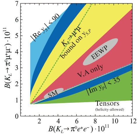
Figure 5: Impact of helicity-allowed tensor and pseudotensor operators in the $\mathcal{B}^{e^{+}e^{-}}$ – $\mathcal{B}^{\mu^{+}\mu^{-}}$ plane of Fig.4. The green area (up to the green dashed line) corresponds to arbitrary $y_{7A,7V}$ together with $\Lambda_{T,\tilde{T}}$ compatible with $\mathcal{B}\left(K^{+}\rightarrow\pi^{+}\nu\bar{\nu}\right)$, as explained in the text.

The forward-backward asymmetry:

The muonic asymmetry $A_{FB}^{\mu}$ can be enhanced only by $Q_{S}$ and $Q_{T}$ contributions, as explained in earlier sections, and this through interferences with $\mathcal{M}_{\mathrm{ICPV}}^{\ast}$ and $\mathcal{M}_{\mathrm{\gamma\gamma-0}^{++}}$, respectively, see Eq.(52). Tuning $y_{7V}$ and the helicity-allowed $1/\bar{\Lambda}_{T}^{2}$ term, a maximum of about $60\%$ can be reached. Still, this requires large contributions from $Q_{T}$ with both $K_{L}\rightarrow\pi^{0}\ell^{+}\ell^{-}$ rates above $10^{-10}$. With $\bar{\Lambda}_{T}\gtrsim 1$, this maximum falls to about $30\%$, i.e. close to the SM value Eq.(26).

For the electronic mode, one could think that a small $\bar{\Lambda}_{S}$ could generate a significant asymmetry through the helicity-allowed interference with $\mathcal{M}_{\mathrm{ICPV}}^{\ast}$. However, this is not the case because the impact of $Q_{S}$ on $\mathcal{B}^{e^{+}e^{-}}$ is then much more pronounced. Tensor interactions, for their parts, have a small impact on $A_{FB}^{e}$ because interference effects with $\mathcal{M}_{\mathrm{2}^{++}}$ are helicity-suppressed.

4 Summary and Conclusion

The $K_{L}\rightarrow\pi^{0}\ell^{+}\ell^{-}$ modes offer a unique opportunity to probe a large range of New Physics $\Delta S=1$ effective operators, see Table 2. They are therefore an essential tool in the investigation of flavor structures beyond the Standard Model. Our work was to analyze, in a model-independent way, the possible experimental signatures of these New Physics interactions.

$\begin{array}[c]{c}\text{Short-distance}\\ \text{operator}\end{array}$ $\begin{array}[c]{c}\text{CP-property}\\ \text{\& }J^{PC}\left(\bar{\ell}\ell\right)\end{array}$ $\begin{array}[c]{c}\text{Helicity-}\\ \text{suppressed}\end{array}$ $\begin{array}[c]{c}\text{Helicity-}\\ \text{allowed}\end{array}$ ICPV ($K^{0}$-$\bar{K}^{0}$) – CPV ($1^{--}$) Eq.(12) Two-photon – CPC ($0^{++}$) Eq.(12) Vector $(\bar{s}\gamma_{\mu}d)(\bar{\ell}\gamma^{\mu}\ell)$ CPV ($1^{--}$) Eq.(12) Axial-vector $(\bar{s}\gamma_{\mu}d)(\bar{\ell}\gamma^{\mu}\gamma_{5}\ell)$ CPV ($0^{-+},1^{++}$) Eq.(12) Pseudoscalar $\left(\bar{s}d\right)\left(\bar{\ell}\gamma_{5}\ell\right)$ CPV ($0^{-+}$) Eq.(36) Eq.(55) Scalar $\left(\bar{s}d\right)\left(\bar{\ell}\ell\right)$ CPC ($0^{++}$) Eq.(39) Eq.(55) Tensor $\left(\bar{s}\sigma_{\mu\nu}d\right)\left(\bar{\ell}\sigma^{\mu\nu}\ell\right)$ CPV ($1^{--}$) Eq.(48) Eq.(55) Pseudotensor $\left(\bar{s}\sigma_{\mu\nu}d\right)\left(\bar{\ell}\sigma^{\mu\nu}\gamma_{5}\ell\right)$ CPC ($1^{+-}$) Eq.(51) Eq.(55)

Table 2: Summary of the contributions entering the $K_{L}\rightarrow\pi^{0}\ell^{+}\ell^{-}$ rate, and references to the relevant formulas in the text. The CP-property indicates which of the real or imaginary part of the respective Wilson coefficient contributes. Interferences occur whenever the $\bar{\ell}\ell$ pair is produced in the same state. ‘Helicity-suppressed/allowed’ refers to the last four operators.

In the presence of vector and axial-vector interactions only, the two rates are bounded in the $\mathcal{B}^{e^{+}e^{-}}$–$\mathcal{B}^{\mu^{+}\mu^{-}}$ plane (see Fig.5), i.e., at $1\sigma$,

$$0.1\cdot 10^{-11}+0.24\mathcal{B}_{\mathrm{V,A}}^{e^{+}e^{-}}<\mathcal{B}_{\mathrm{V,A}}^{\mu^{+}\mu^{-}}<0.6\cdot 10^{-11}+0.58\mathcal{B}_{\mathrm{V,A}}^{e^{+}e^{-}}\;.$$ (58)

Any signal outside this region is an indication of New Physics FCNC operators of different structures (baring the possibility of large $\mu-e$ universality breaking in the V,A currents). We have identified two possible mechanisms.

The first is from helicity-suppressed (pseudo-)scalar operators, as arising in the MSSM at large $\tan\beta$. These enhance the muonic mode without affecting the electronic mode. Such interactions would be revealed by measuring the two rates above the V,A region. Also, comparing with $K_{L}\rightarrow\mu^{+}\mu^{-}$ shows, model-independently, that the $K_{L}\rightarrow\pi^{0}\mu^{+}\mu^{-}$ is more sensitive (besides being cleaner) to these types of interactions (see the yellow region in Fig.5).

The second possibility is from helicity-allowed (pseudo-)tensor interactions, which could arise for example from tree-level leptoquark interactions. Because of the phase-space suppression, it is now the electronic mode which is more affected. These interactions would manifest themselves in a signal significantly below the V,A region (see the green region in Fig.5). Even assuming the presence of similar contributions for the $K\rightarrow\pi\nu\bar{\nu}$ modes, there is at present no severe constraint on these effects.

On the other hand, we found that both helicity-suppressed (pseudo-)tensor interactions and helicity-allowed (pseudo-)scalar interactions should not lead to observable effects. For the former, this is so because of significant phase-space suppression, while the latter are already strongly bounded by the very rare $K_{L}\rightarrow e^{+}e^{-}$ decay. Also, concerning the electromagnetic tensor operator, $\left(\bar{s}\sigma_{\mu\nu}d\right)F^{\mu\nu}$, measurements of the $K_{L}\rightarrow\pi^{0}\ell^{+}\ell^{-}$ rates cannot disentangle it from vector operator contributions.

For the (integrated) forward-backward asymmetry $A_{FB}^{\mu}$, the first reliable estimate has been obtained. It is typically of a few tens of percents, and can give important information, complementary to the total rates. In the SM, it could fix the sign of the interference between the vector operator and ICPV contributions. Similarly, beyond the SM, it can be used to discriminate among various solutions once both $K_{L}\rightarrow\pi^{0}\ell^{+}\ell^{-}$ rates are measured. On the other hand, the electronic asymmetry $A_{FB}^{e}$ is found either completely dominated by its (unknown) SM value, or too small to be of any use to constrain either New Physics or $a_{S}$.

We have not included differential rates or differential asymmetries in the present study (though they can be trivially computed from our analyses). New physics does affect these observables, but they require a higher experimental sensitivity, so total rates and integrated asymmetries are more promising.

With the general expressions for both $K_{L}\rightarrow\pi^{0}\ell^{+}\ell^{-}$ rates and asymmetries computed in Sections 2 and 3, the way is now paved for more model-dependent analyses. In this context, the $\mathcal{B}^{e^{+}e^{-}}$–$\mathcal{B}^{\mu^{+}\mu^{-}}$ plane remains as a particularly convenient phenomenological tool to display the correlations among operators specific to a given model.

In conclusion, the $K_{L}\rightarrow\pi^{0}\ell^{+}\ell^{-}$ system, together with the neutrino modes $K\rightarrow\pi\nu\bar{\nu}$, has a considerable potential for unveiling/constraining the nature of possible New Physics in $\Delta S=1$ FCNC, therefore playing an important role in the quest for a better understanding of the quark flavor sector.

Acknowledgements

We are pleased to thank Gino Isidori for stimulating discussions and for reading the manuscript, and Paride Paradisi for useful comments. This work is partially supported by IHP-RTN, EC contract No. HPRN-CT-2002-00311 (EURIDICE). The work of C.S. is also supported by the Schweizerischer Nationalfonds; S.T. acknowledges the support of the DFG grant No. NI 1105/1-1.

Appendix A Constraints on (pseudo-)scalar operators from $K_{L}\rightarrow\mu^{+}\mu^{-}$

We consider the following effective Hamiltonian:

$$\mathcal{H}_{eff}=\frac{G_{F}\alpha}{\sqrt{2}}\lambda_{t}y_{7A}^{\prime}\left(\bar{s}\gamma_{\mu}\gamma_{5}d\right)\left(\bar{\ell}\gamma^{\mu}\gamma_{5}\ell\right)+\frac{G_{F}^{2}M_{W}^{2}}{\pi^{2}}\frac{m_{s}m_{\ell}}{M_{W}^{2}}\left[y_{P}^{\prime}\left(\bar{s}\gamma_{5}d\right)\left(\bar{\ell}\gamma_{5}\ell\right)+y_{S}^{\prime}\left(\bar{s}\gamma_{5}d\right)\left(\bar{\ell}\ell\right)\right]+h.c.$$ (59)

In the SM, $y_{7A}^{\prime}=y_{7A}$ and $y_{P,S}^{\prime}$ are negligible. Our goal is to get an order of magnitude estimate of the bounds set on $y_{P,S}^{\prime}$ by the measured $K_{L}\rightarrow\mu^{+}\mu^{-}$ rate.

Using the matrix element parametrizations

$$\langle 0|\bar{s}\gamma_{\mu}\gamma_{5}d|K^{0}\left(P\right)\rangle=i\sqrt{2}F_{K}P_{\mu},\;\;\langle 0|\bar{s}\gamma_{5}d|K^{0}\rangle=-i\sqrt{2}F_{K}\frac{M_{K}^{2}}{m_{s}+m_{d}}\;,$$ (60)

in the same conventions as Eq.(9), the decay amplitudes $\langle\ell^{+}\ell^{-}|-\mathcal{H}_{eff}|K_{L,S}\rangle$ and the total rates can be written as

$$\mathcal{M}\left(K_{L,S}\rightarrow\ell^{+}\ell^{-}\right) =2i\frac{G_{F}^{2}M_{W}^{2}F_{K}M_{K}}{\pi^{2}}r_{\ell}\left\{\bar{u}_{p}\left(A_{L,S}^{\ell}+B_{L,S}^{\ell}\gamma_{5}\right)v_{p^{\prime}}\right\}\;,$$ (61)

$$\Gamma\left(K_{L,S}\rightarrow\ell^{+}\ell^{-}\right) =\frac{G_{F}^{4}M_{W}^{4}F_{K}^{2}M_{K}^{3}}{2\pi^{5}}r_{\ell}^{2}\sqrt{1-4r_{\ell}^{2}}\left(\left(1-4r_{\ell}^{2}\right)\left|A_{L,S}^{\ell}\right|^{2}+\left|B_{L,S}^{\ell}\right|^{2}\right)\;,$$ (62)

with $A_{S},B_{L}$ ($A_{L},B_{S}$) the CP-conserving (CP-violating) pieces given by

$$A_{L}^{\ell} =\frac{M_{K}^{2}}{M_{W}^{2}}i\operatorname{Im}y_{S}^{\prime},\;B_{L}^{\ell}=\frac{M_{K}^{2}}{M_{W}^{2}}\operatorname{Re}y_{P}^{\prime}-\left(2\pi\sin^{2}\theta_{W}\right)\left(\operatorname{Re}\left(\lambda_{t}y_{7A}^{\prime}\right)+\operatorname{Re}\lambda_{c}y_{c}\right)+A_{L\gamma\gamma}^{\ell}\;,$$ (63)

$$A_{S}^{\ell} =\frac{M_{K}^{2}}{M_{W}^{2}}\operatorname{Re}y_{S}^{\prime}+A_{S\gamma\gamma}^{\ell},\;B_{S}^{\ell}=\frac{M_{K}^{2}}{M_{W}^{2}}i\operatorname{Im}y_{P}^{\prime}-\left(2\pi\sin^{2}\theta_{W}\right)i\operatorname{Im}\left(\lambda_{t}y_{7A}^{\prime}\right)\;.$$ (64)

The $c$-quark contribution is negligible for $K_{S}\rightarrow\mu^{+}\mu^{-}$, while for $K_{L}\rightarrow\mu^{+}\mu^{-}$, it has been computed recently to NNLO giving $y_{c}=\left(-2.0\pm 0.3\right)\cdot 10^{-4}$[42]. Indirect CPV contributions are understood, $\mathcal{M}\left(K_{L,S}\rightarrow\ell^{+}\ell^{-}\right)_{\mathrm{ICPV}}=\varepsilon\mathcal{M}\left(K_{1,2}\rightarrow\ell^{+}\ell^{-}\right)$.

The two-photon term $A_{S\gamma\gamma}^{\ell}$ is given in [19] in terms of the two-loop form-factor of Eq.(5):

$$A_{S\gamma\gamma}^{\mu}=-\frac{\alpha_{em}^{2}G_{8}F_{\pi}}{2G_{F}^{2}M_{W}^{2}F_{K}}\left(1-r_{\pi}^{2}\right)\mathcal{I}\left(r_{\mu}^{2},r_{\pi}^{2}\right)=2.10\cdot 10^{-4}\left(-2.821+i1.216\right)\;.$$ (65)

For $K_{L}$, the situation is less clear as the dispersive part of $A_{L\gamma\gamma}^{\ell}$ is notoriously difficult to evaluate. Anyway, following the analysis of Ref.[4], one can get the conservative estimate

$$A_{L\gamma\gamma}^{\mu}=\sqrt{\frac{4\pi^{3}\alpha_{em}^{2}\Gamma\left(K_{L}\rightarrow\gamma\gamma\right)}{G_{F}^{4}F_{K}^{2}M_{W}^{4}M_{K}^{3}}}\left(\chi_{disp}+i\chi_{abs}\right)=\pm 1.98\cdot 10^{-4}\left(\left(0.71\pm 0.15\pm 1.0\right)-i5.21\right)\;.$$ (66)

The sign of this contribution depends on the sign of the $K_{L}\rightarrow\gamma\gamma$ amplitude[4], itself depending on the sign of an unknown low-energy constant (see [21]).

To get an order-of-magnitude estimate of the coefficients, we allow for both signs in the $K_{L}\rightarrow\mu^{+}\mu^{-}$ branching ratio

$$\mathcal{B}\left(K_{L}\rightarrow\mu^{+}\mu^{-}\right)=\left(6.7+\left(0.08\operatorname{Im}y_{S}^{\prime}\right)^{2}+\left(0.10\operatorname{Re}y_{P}^{\prime}+1.1y_{7A}^{\prime}-0.2\pm 0.4_{-0.5}^{+0.5}\right)^{2}\right)\cdot 10^{-9}\;,$$ (67)

and reflect only the error on $\chi_{disp}$. Then, imposing the rate to be within $3\sigma$ of the experimental value $\mathcal{B}\left(K_{L}\rightarrow\mu^{+}\mu^{-}\right)^{\exp}=\left(6.87\pm 0.12\right)\cdot 10^{-9}$[22] corresponds to $\left|\operatorname{Im}y_{S}^{\prime}\right|\lesssim 8$ and $\left|\operatorname{Re}y_{P}^{\prime}\right|\lesssim 35$ for the SM value $y_{7A}^{\prime}=-0.68$. Relaxing this latter constraint to $\left|y_{7A}^{\prime}\right|\lesssim 3$ corresponds to $\left|\operatorname{Re}y_{P}^{\prime}\right|\lesssim 70$, much larger since the two interfere in the rate.

For $K_{S}\rightarrow\mu^{+}\mu^{-}$, the experimental bound $\mathcal{B}\left(K_{S}\rightarrow\mu^{+}\mu^{-}\right)^{\exp}<3.2\cdot 10^{-7}$ is still very far from the predicted rate of about $4\cdot 10^{-12}$ in the SM. Taking $\left|\operatorname{Re}y_{S}^{\prime}\right|,\left|\operatorname{Im}y_{P}^{\prime}\right|\lesssim 50$ cannot enhance the branching ratio beyond $\mathcal{B}\left(K_{S}\rightarrow\mu^{+}\mu^{-}\right)\lesssim 10^{-10}$.

Finally, for completeness, the longitudinal muon polarization in $K_{L}\rightarrow\mu^{+}\mu^{-}$ is expressed as [43]

$$P_{L}=\frac{2\sqrt{1-4r_{\mu}^{2}}\operatorname{Im}\left(B_{L}^{\mu\,\ast}A_{L}^{\mu}\right)}{\left(1-4r_{\mu}^{2}\right)\left|A_{L}^{\mu}\right|^{2}+\left|B_{L}^{\mu}\right|^{2}}\;.$$ (68)

In the SM, this quantity is entirely driven by the indirect CP-violating contribution, proportional to $\varepsilon$, and is thus rather small, $|P_{L}|\sim 2\times 10^{-3}$[19]. Including the scalar and pseudoscalar currents, we find that for $\left|\operatorname{Re}y_{P}^{\prime}\right|,\left|\operatorname{Im}y_{P}^{\prime}\right|\lesssim 75$, only a 10% deviation of $P_{L}$ from its SM value can be generated. On the other hand, $\left|\operatorname{Re}y_{S}^{\prime}\right|\lesssim 75$ can enhance $\left|P_{L}\right|$ up to about $10^{-2}$, while for $\left|\operatorname{Im}y_{S}^{\prime}\right|\lesssim 8$, $\left|P_{L}\right|$ can be as large as $8\%$. It is indeed this latter parameter which is the most important since it does not require any $\varepsilon$ factor. This makes $P_{L}$ particularly sensitive to the presence of new CP-violating sources in the scalar operator (as discussed e.g. in [44]). Unfortunately, a percent level measurement of $P_{L}$ in the medium term is unlikely, and the $K_{L}\rightarrow\pi^{0}\mu^{+}\mu^{-}$ total rate is more promising to get a signal or set limits on these New Physics interactions.

Appendix B Numerical representation of the two-loop form factor

In Refs.[19, 3], the two-loop form-factor is expressed as a complicated three-dimensional integral. For practical purposes, the following numerical representations can be used instead:

$$\mathcal{I}\left(\frac{r_{\ell}^{2}}{z},\frac{r_{\pi}^{2}}{z}\right) =\left\{\begin{array}[c]{l}\sum_{k=0}^{5}a_{k}^{\ell}\left(0.33-z\right)^{-k/2},\;\;0\leqslant z<0.315\,,\\ \sum_{k=0}^{5}b_{k}^{\ell}\left(z-0.30\right)^{-k/2},\;\;0.315\leqslant z\lesssim 0.6\;,\end{array}\right.$$

$$\mathcal{I}\left(\frac{r_{\ell}^{2}}{z},\frac{1}{z}\right) =\sum_{k=0}^{5}c_{k}^{\ell}\left(1-z\right)^{-k/2},\;0\leqslant z\lesssim 0.6\;,$$

with

$$k$$

      

$$k$$

      

Using this parametrization, one can reproduce the rates and asymmetries typically with an error of about one percent, which is more than sufficient given the size of the theoretical uncertainty on the $a_{1}^{P}\left(z\right)$ distributions.

References

[1]G. D’Ambrosio, G. Ecker, G. Isidori, J. Portoles, JHEP
08 (1998) 004.
[2]G. Buchalla, G. D’Ambrosio and G. Isidori, Nucl. Phys.
B672 (2003) 387.
[3]G. Isidori, C. Smith and R. Unterdorfer, Eur.
Phys. J. C36 (2004) 57.
[4]G. Isidori and R. Unterdorfer, JHEP 0401 (2004) 009.
[5]K. S. Babu and C. F. Kolda, Phys. Rev. Lett. 84
(2000) 228; A. Dedes and A. Pilaftsis, Phys. Rev. D67 (2003) 015012;
C. Hamzaoui, M. Pospelov and M. Toharia, Phys. Rev. D59 (1999)
095005; A. Dedes, Mod. Phys. Lett. A18 (2003) 2627.
[6]J. Foster, K. I. Okumura and L. Roszkowski, Phys. Lett.
B609 (2005) 102.
[7]T. Banks, Y. Grossman, E. Nardi and Y. Nir, Phys. Rev.
D52 (1995) 5319; K. Agashe and M. Graesser, Phys. Rev. D54
(1996) 4445; G. Bhattacharyya and A. Raychaudhuri, Phys. Rev. D57
(1998) 3837; R. Barbier et al., hep-ph/9810232; A. Deandrea,
J. Welzel and M. Oertel, JHEP 0410 (2004) 038; M. Chemtob, Prog.
Part. Nucl. Phys. 54 (2005) 71.
[8]S. Davidson, D. C. Bailey and B. A. Campbell, Z. Phys.
C61 (1994) 613.
[9]A. J. Buras, G. Colangelo, G. Isidori, A. Romanino and
L. Silvestrini, Nucl. Phys. B566 (2000) 3.
[10]G. D’Ambrosio and D. N. Gao, JHEP 0207 (2002) 068.
[11]L.M. Sehgal, Phys. Rev. D38 (1988) 808; P. Heiliger and
L.M. Sehgal, Phys. Rev. D47 (1993) 4920; J. F. Donoghue and F.
Gabbiani, Phys. Rev. D51 (1995) 2187.
[12]M. V. Diwan, H. Ma, T. L. Trueman, Phys. Rev. D65
(2002) 054020; D. N. Gao, Phys. Lett. B586 (2004) 307.
[13]G. Buchalla, A. J. Buras and M. E. Lautenbacher, Rev.
Mod. Phys. 68 (1996) 1125.
[14]P. L. Cho, M. Misiak and D. Wyler, Phys. Rev. D54
(1996) 3329; A. J. Buras, P. Gambino, M. Gorbahn, S. Jager and L. Silvestrini,
Nucl. Phys. B592 (2001) 55; G. Isidori, F. Mescia, P. Paradisi, C.
Smith and S. Trine, hep-ph/0604074.
[15]G. Isidori and P. Paradisi, Phys. Rev. D73
(2006) 055017.
[16]A. J. Buras and L. Silvestrini, Nucl. Phys. B546
(1999) 299.
[17]A. J. Buras, R. Fleischer, S. Recksiegel and F. Schwab, Nucl.
Phys. B697 (2004) 133.
[18]J. R. Batley et al. [NA48/1 Collaboration], Phys.
Lett. B576 (2003) 43; Phys. Lett. B599 (2004) 197.
[19]G. Ecker and A. Pich, Nucl. Phys. B366 (1991) 189.
[20]A. Alavi-Harati et al. [KTeV Collaboration], Phys.
Rev. Lett. 83 (1999) 917; A. Lai et al. [NA48 Collaboration], Phys.
Lett. B536 (2002) 229.
[21]J.-M. Gérard, C. Smith and S. Trine, Nucl. Phys.
B730 (2005) 1.
[22]Particle Data Group: S. Eidelman et al., Phys. Lett.
B592 (2004) 1, and 2005 partial update for edition 2006.
[23]T. Alexopoulos et al. [KTeV Collaboration],
Phys. Rev. D70 (2004) 092007; A. Lai et al. [NA48
Collaboration], Phys. Lett. B604 (2004) 1; O. P. Yushchenko
et al., Phys. Lett. B581 (2004) 31; F. Ambrosino
et al. [KLOE Collaboration], Phys. Lett. B636 (2006) 166.
[24]W.J. Marciano and Z. Parsa, Phys. Rev. D53
(1996) 1.
[25]H. Leutwyler and M. Roos, Z. Phys. C25 (1984) 91.
[26]C. Dawson, T. Izubuchi, T. Kaneko, S. Sasaki and A. Soni,
PoS LAT2005 (2006) 337; N. Tsutsui et al. [JLQCD
Collaboration], PoS LAT2005 (2006) 357; M. Okamoto [Fermilab Lattice
Collaboration], hep-lat/0412044; D. Becirevic et al.,
Nucl. Phys. B705 (2005) 339.
[27]S. Friot, D. Greynat and E. de Rafael, Phys. Lett.
B595 (2004) 301.
[28]J. Charles et al. [CKMfitter Group], Eur. Phys.
J. C41 (2005) 1, and Aug. 1, 2005 updated results presented at EPS
2005, Lisbon, Portugal.
[29]A. Alavi-Harati et al. [KTeV Collaboration], Phys.
Rev. Lett. 93 (2004) 021805.
[30]A. Alavi-Harati et al. [KTEV Collaboration],
Phys. Rev. Lett. 84 (2000) 5279.
[31]L. Michel, Proc. Phys. Soc. A63 (1950) 514.
[32]C. Bobeth, A. J. Buras, F. Kruger and J. Urban, Nucl. Phys.
B630 (2002) 87.
[33]G. Isidori and A. Retico, JHEP 0111 (2001)
001; JHEP 0209 (2002) 063.
[34]M. Ciuchini et al., JHEP 9810 (1998) 008.
[35]A. J. Buras, M. Misiak and J. Urban, Nucl. Phys. B586
(2000) 397; M. Ciuchini, E. Franco, V. Lubicz, G. Martinelli, I. Scimemi and
L. Silvestrini, Nucl. Phys. B523 (1998) 501.
[36]S. Fukae, C. S. Kim, T. Morozumi and T. Yoshikawa, Phys.
Rev. D59 (1999) 074013; T. M. Aliev, V. Bashiry and M. Savci, Phys.
Rev. D73 (2006) 034013.
[37]D. Becirevic, V. Lubicz, G. Martinelli and F. Mescia, Phys.
Lett. B501 (2001) 98.
[38]G. Colangelo, G. Isidori and J. Portoles, Phys. Lett.
B470 (1999) 134.
[39]L. Littenberg, Lectures given at PSI Zuoz Summer School on
Exploring the Limits of the Standard Model, Zuoz, Switzerland, 18-24 Aug 2002,
hep-ex/0212005.
[40]A. J. Buras, M. Gorbahn, U. Haisch and U. Nierste, Phys.
Rev. Lett. 95 (2005) 261805; hep-ph/0603079.
[41]S. Adler et al. [E787], Phys. Rev. Lett.
88 (2002) 041803; V. V. Anisimovsky et al. [E949], Phys.
Rev. Lett. 93 (2004) 031801.
[42]M. Gorbahn and U. Haisch, hep-ph/0605203.
[43]P. Herczeg, Phys. Rev. D27 (1983) 1512.
[44]S. R. Choudhury, N. Gaur and A. Gupta, Phys. Lett.
B482 (2000) 383.