$K^{L}_{\mu 3}$ decay: A Stringent Test of Right-Handed Quark Currents

Véronique Bernard ^a,, Micaela Oertel ^b,, Emilie Passemar ^c, and Jan Stern ^c,

^a Université Louis Pasteur, Laboratoire de Physique Théorique,

3-5 rue de l’Université, F-67084 Strasbourg, France
^b LUTH, Observatoire de Paris, F-92195 Meudon, France

^c Groupe de Physique Théorique, IPN, Université de Paris Sud-XI, F-91406 Orsay, France

Abstract: Clean tests of a small admixture of right-handed quark currents directly coupled to the standard $W$ are still lacking. We show that such non-standard couplings can be signifi-cantly constrained measuring the value of the scalar $K\pi$ form factor at the Callan-Treiman point to a few percent. A realistic prospect of such a measurement in $K^{L}_{\mu 3}$ decay based on an accurate dispersive representation of the scalar form factor is presented. The inadequacy of the currently used linear parametrisation is explained and illustrated using recent KTeV data. We briefly comment on the charged Kaon mode.

I. In this letter we propose a new dedicated test of (the absence of) charged right-handed currents (RHCs) involving light quarks. We show how high statistics measurements [1, 2] of Dalitz distributions in the $K^{L}_{\mu 3}$ decay, $K_{L}\to\pi^{\pm}\mu^{\mp}\nu$, can be used to extract the value $\mathrm{C}=f(\Delta_{K\pi})$ of the scalar $K\pi$ form factor at the Callan-Treiman point $\Delta_{K\pi}=m_{K^{0}}^{2}-m_{\pi^{+}}^{2}$ and how this information constrains the effect of $\bar{u}d$ and $\bar{u}s$ RHCs. The method is model independent. It is based on the observation that standard dispersive technics and the known low-energy $K\pi$ phases lead to an accurate parametrization of the scalar $K\pi$ form factor in terms of a single parameter $\mathrm{C}$ subject to experimental determination. The related theoretical uncertainties are under control and they remain small compared with the possible signal of RHCs. We will comment on charged K-decays shortly in section VI.

II. In the past, tests of RHCs have often been considered in connection with left-right symmetric extensions of the Standard Model (SM) [3], yielding a lower bound on the mass $M_{W_{R}}$ of the hypothetical vector boson mediating the RH weak interactions [4]. Different models leading to RHCs through mixing with heavy exotic fermions [5] have been considered, too. Independently of any specific models, RHCs naturally arise in Low Energy Effective Theories which below some scale $\Lambda_{W}$ operate with SM degrees of freedom and symmetries. Such RHC interactions are not necessarily mediated by an extra gauge boson $W_{R\mu}$ and they need not be concerned by phenomenological lower bounds on $M_{W_{R}}$. Indeed, there exists a unique $\mathrm{SU}(2)\times\mathrm{U(1)}$ gauge-invariant operator [6]

$$O_{\mathrm{RHC}}=\frac{1}{\Lambda^{2}}(\bar{U}_{R}\gamma^{\mu}D_{R})\phi_{r}\epsilon^{rs}(D_{\mu}\phi)_{s}$$ (1)

describing a direct coupling of $W^{\mu}$ with the RHC $\bar{U}_{R}\gamma_{\mu}D_{R}$. The presence of the Higgs doublet $\phi_{r}(r=1,2)$ in Eq. (1) suggests that the actual strength of this operator depends on the mechanism of electroweak symmetry breaking.
If the symmetry is linearly realized and the light Higgs particle exists, the operator Eq. (1) is just one among the 80 independent gauge invariant operators of the mass (or UV) dimension $D=6$ [6] and it is not easy to disentangle their respective dimensional suppression.
In the opposite case of a Higgs-less effective theory [7, 8], only the three Goldstone bosons contained in the complex Higgs doublet $\phi_{r}$ remain in Eq. (1) and the operator $O_{\mathrm{RHC}}$ becomes of the chiral (infrared) dimension $d=2$, i.e., it is not dimensionally suppressed anymore. Instead, its suppression is now related to its symmetry properties with respect to the higher non-linearly realized gauge symmetry characteristic of Higgsless vertices of the SM [7]. As a result the RHC interaction now appears already at the NLO: it represents a genuine effect beyond the SM that is potentially more important than the loop corrections. In the framework of a systematic low-energy expansion, one should first consider observables that are linear in the operator Eq. (1) (or in its Higgs-less analogue given in [7]).
There exists a compelling experimental evidence against charged RHCs in the lepton sector based on polarisation measurements in $\mu$-decay, $\tau$-decay and $\beta$-decay [4, 9]. Recent findings on neutrino mixings and masses however suggest that quark and lepton sectors and, in particular, the corresponding RHCs interactions need not be alike. If the right (Majorana) neutrino is heavy compared to the scale $\Lambda_{W}$ of the Effective theory, there will be no RHCs visible at low energy. In the opposite case, the lepton sector should enjoy an extra symmetry (not present for quarks) that suppresses the neutrino Dirac mass and thereby the leptonic charged RHCs as well [7]. (The simplest example of such a discrete symmetry is the $\nu_{R}$ sign flip symmetry $\nu_{R}\to-\nu_{R}$ introduced in [7].) Notice that the disymmetry between quark and lepton couplings beyond the leading order would generate an anomaly which in the Effective theory is compensated by the Wess-Zumino term constructed in [11]. In particular, there does not seem to be any obvious consistency or plausibility argument against the quark charged RHCs Eq. (1) even if the latter is absent for leptons.
Surprisingly enough the available experimental constraints on first order RHC effects of quarks remain so far rather meagre. They suffer either from the lack of precision or from the excess of model dependence facing non-perturbative QCD effects. Global fits to electroweak precision data based on electroweak effective Lagrangians [12] usually do not strongly constrain the operator Eq. (1). Some time ago, the CDHS collaboration has reported a dedicated test of RHCs, later confirmed by CCFR [13], based on the $\mathrm{y}$-dependence of $\nu(\bar{\nu})$ DIS off valence quarks. Unfortunately, only the square of the RHC operator, Eq. (1), contributes to the leading twist. Such contribution of RHCs is strongly suppressed and it can be hardly disentangled from higher twist left-handed contributions. It has been further observed that a RHC interaction would alter the chiral structure of the tree-level effective weak Hamiltonian and the corresponding consequences of soft-pion theorems for weak $K$ and hyperon decays [14] in an experimentally relevant way. However, the upper bounds on RHCs derived from this observation did not consider long distance chiral loop corrections (such as final state interaction) which are known to be rather important and can easily upset small tree-level effects. The strongest constraint on left-right symmetric models is known to arise from the $W_{R\mu}$-exchange contribution to the $K^{0}-\bar{K}^{0}$ mixing [19]. However, in an effective theory where a (light) $W_{R\mu}$ is absent, the leading RHC effect arises from the $\bar{s}d\leftrightarrow\bar{d}s$ box diagram with an insertion of a single RHC vertex Eq. (1). Due to Lorentz invariance, the resulting four-fermion operator in $H_{W}^{\Delta S=2}$ necessarily involves derivatives and it is suppressed by the external momentum scale in addition to the suppression by the small coefficient of the operator in Eq. (1). A similar argument applies to $\Delta S=1$ FCNC such as $K\rightarrow\pi\nu\bar{\nu}$. All such contributions of RHCs to FCNC processes are expected to be smaller than in the SM.

It is convenient to write the effective CC interaction vertex in a matrix notation

$${\cal L}_{CC}=\tilde{g}[l_{\mu}+\frac{1}{2}\bar{\mathrm{U}}({\cal V}_{eff}\gamma_{\mu}+{\cal A}_{eff}\gamma_{\mu}\gamma_{5})\mathrm{D}]W^{\mu}+h.c.\ ,\,\mathrm{U}=\begin{pmatrix}u\\ c\\ t\end{pmatrix},\,\mathrm{D}=\begin{pmatrix}d\\ s\\ b\end{pmatrix},$$ (2)

and ${\cal V}_{eff}$, ${\cal A}_{eff}$ are complex $3\times 3$ effective coupling matrices. In the Standard Model one has

$${\cal V}_{eff}=-{\cal A}_{eff}=V_{CKM},$$ (3)

where $V_{CKM}$ is the unitary flavour mixing matrix. Recently, much effort has been devoted to experimentally test the unitarity of $V_{CKM}$. The issue of such tests usually depends on the stage of our theoretical knowledge of corresponding hadronic matrix elements. For instance, in the case of light quark elements $V^{ud}$ and $V^{us}$ the CKM unitarity is not yet established: whereas lattice calculations of the $K_{e3}$ decay form factor $f_{+}(0)$ [15] are compatible with the first row of CKM unitarity, the two-loop $\chi PT$ calculation [16] indicates a possible violation of the latter by as much as $2.6\leavevmode\nobreak\ \sigma$ [17]. Furthermore, there is practically no significant test of the relation ${\cal V}_{eff}=-{\cal A}_{eff}$, i.e. of the absence of RHCs. There is an intermediate step between the SM case Eq. (3) and the completely general effective couplings Eq. (2). The departure from the SM can still be universal up to and including the NLO, meaning that there exists a chiral flavour basis in which both ${\cal V}_{eff}$ and ${\cal A}_{eff}$ are proportional to the unit matrix. (In other words, all flavor symmetry breaking can be transformed from vertices to the mass matrix.) This property is shared by many models with minimal flavor violation [18]. It can be equivalently expressed in terms of effective couplings as ($i=u,c,t;j=d,s,b$)

$${\cal V}_{eff}^{ij}=(1+\delta)V_{L}^{ij}+\epsilon V_{R}^{ij}+\mathrm{NNLO}\,,\hskip 28.45274pt{\cal A}_{eff}^{ij}=-(1+\delta)V_{L}^{ij}+\epsilon V_{R}^{ij}+\mathrm{NNLO}.$$ (4)

Here, $\delta$ and $\epsilon$ are two small parameters measuring the departure from the SM , whereas $V_{L}$ and $V_{R}$ are two a priori independent unitary matrices arising from the diagonalisation of the generic quark mass matrix. As already discussed, we do not introduce charged leptonic RHCs: in Eq. (2) $l_{\mu}$ stands for the standardly normalized V-A lepton current. A few direct first order constraints on the parameters $\epsilon$ and $\delta$ at the percent level are conceivable. They can be obtained from selected tree-level semi-leptonic processes in which QCD effects are under theoretical control. This is true, in particular, for inclusive hadronic $\tau$-decays whose impact on the parameters $\epsilon$ and $\delta$ will be discussed separately [28]. Here, we concentrate on the $K_{\mu 3}$ decay which could provide one of the most stringent probes of RHCs. To the best of our knowledge, none of these tests has been considered previously.

III. We consider the hadronic matrix element describing the $K^{0}_{\mu 3}$ decay:

$$\langle\pi^{-}(p^{\prime})|\bar{s}\gamma_{\mu}u|K^{0}(p)\rangle=(p^{\prime}+p)_{\mu}\ f^{K^{0}\pi^{-}}_{+}(t)+(p-p^{\prime})_{\mu}\ f_{-}^{K^{0}\pi^{-}}(t),$$ (5)

where $t=(p^{\prime}-p)^{2}=(p_{\mu}+p_{\nu})^{2}$. The vector form factor $f^{K^{0}\pi^{-}}_{+}(t)$ represents the P-wave projection of the crossed channel matrix element $\langle 0|\bar{s}\gamma_{\mu}u|K\pi\rangle$, whereas the S-wave projection is described by the scalar form factor:

$$f_{S}(t)=f^{K^{0}\pi^{-}}_{+}(t)+\frac{t}{m^{2}_{K^{0}}-m^{2}_{\pi^{-}}}f^{K^{0}\pi^{-}}_{-}(t).$$ (6)

In the experimental study of decay distributions one usually factorizes from both form factors $f^{K^{0}\pi^{-}}_{+}(t)$ and $f^{K^{0}\pi^{-}}_{S}(t)$ the common factor $f^{K^{0}\pi^{-}}_{+}(0)$ to normalize them to 1 at $t=0$. We thus concentrate on the normalized scalar form factor

$$f(t)=\frac{f^{K^{0}\pi^{-}}_{S}(t)}{f^{K^{0}\pi^{-}}_{+}(0)}\ \ ,\ \ f(0)=1.$$ (7)

The Callan-Treiman low-energy theorem (CT) [20] fixes the value of $f(t)$ at the point $t=\Delta_{K\pi}=m_{K^{0}}^{2}-m_{\pi^{+}}^{2}$ in the $\mathrm{SU}(2)\times\mathrm{SU}(2)$ chiral limit. We can write

$$\mathrm{C}=f(\Delta_{K\pi})=\frac{F_{K^{+}}}{F_{\pi^{+}}}\frac{1}{f_{+}^{K^{0}\pi^{-}}(0)}+\Delta_{CT},$$ (8)

where the CT discrepancy $\Delta_{CT}$ defined by Eq. (8) is expected to be small and eventually calculable in $\chi PT$. It is proportional to $m_{u}$ and/or $m_{d}$. In the limit $m_{d}=m_{u}$ at the NLO in $\chi PT$ one has for the CT discrepancy $\Delta_{CT}^{\mathrm{NLO}}=-3.5\times 10^{-3}$ [21]. We will come back to it in section IV.
As a next step, we express $\mathrm{C}=f(\Delta_{K\pi})$ in terms of measured branching ratios and of the CC effective couplings defined in Eq. (4). From the branching ratio Br $\frac{\displaystyle K^{+}_{l2}(\gamma)}{\displaystyle\pi^{+}_{l2}(\gamma)}$ [22], one gets

$$\Bigl{|}{\frac{F_{K^{+}}{\cal A}_{eff}^{us}}{F_{\pi^{+}}{\cal A}_{eff}^{ud}}}\Bigr{|}^{2}=0.07602(23)(27),$$ (9)

whereas the weighted average of the 3 compatible most recent measurements of the inclusive decay rate $K^{L}_{e3}(\gamma)$ by KTeV [23], NA48 [24], and KLOE [25] leads to

$$|f_{+}^{K^{0}\pi^{-}}(0){\cal V}_{eff}^{us}|=0.21619(55).$$ (10)

The expression for C can now be rewritten as:

$$\mathrm{C}=B_{exp}\leavevmode\nobreak\ r+\Delta_{CT}\leavevmode\nobreak\ .$$ (11)

The branching ratio $B_{exp}=\Bigl{|}\frac{F_{K^{+}}{\cal A}_{eff}^{us}}{F_{\pi^{+}}{\cal A}_{eff}^{ud}}\Bigr{|}\frac{1}{|f_{+}^{K^{0}\pi^{-}}(0){\cal V}_{eff}^{us}|}|{\cal V}_{eff}^{ud}|$, where $|{\cal V}_{eff}^{ud}|$ is precisely known from superallowed $0^{+}\to 0^{+}$ nuclear $\beta$-decays [26] with the recently updated accuracy [27]

$$|{\cal V}_{eff}^{ud}|=0.97377(26)\leavevmode\nobreak\ ,$$ (12)

is $B_{exp}=1.2418\pm 0.0043$ using Eqs. (9), (10) and (12). The parameter $r$ is given by the RHCs effective couplings

$$r=\Bigl{|}\frac{{\cal A}_{eff}^{ud}{\cal V}_{eff}^{us}}{{\cal V}_{eff}^{ud}{\cal A}_{eff}^{us}}\Bigr{|}=1+2(\epsilon_{S}-\epsilon_{NS})+{\cal O}(\epsilon^{2})\leavevmode\nobreak\ ,$$ (13)

where

$$\epsilon_{NS}=\epsilon\ \mathrm{Re}\Bigl{(}\frac{V_{R}^{ud}}{V_{L}^{ud}}\Bigr{)},\ \ \epsilon_{S}=\epsilon\ \mathrm{Re}\Bigl{(}\frac{V_{R}^{us}}{V_{L}^{us}}\Bigr{)}$$ (14)

represent the strengths of $\bar{u}d$ and $\bar{u}s$ RHCs, respectively. The deviation of $r$ from its SM value $r_{SM}=1$ signalizes the presence of RHCs, i.e., a non-vanishing parameter $\epsilon$. Notice however, that the inverse is not true: RHCs characterized by the mixing matrix $V_{R}$ aligned with the CKM left handed matrix, i.e. $V_{R}=\exp(i\omega)V_{L}$ , would not show up in the parameter $r$ and would escape the detection in $K^{L}_{\mu 3}$ decays.
Using the experimental number for the branching ratio mentionned above one gets:

$$\mathrm{lnC}=0.2166\pm 0.0035+\tilde{\Delta}_{CT}+2(\epsilon_{S}-\epsilon_{NS})+{\cal O}(\epsilon^{2})\leavevmode\nobreak\ ,$$ (15)

where $\tilde{\Delta}_{CT}=\Delta_{CT}/B_{exp}$. We now ask how big the effect of RHCs should be to be seen measuring $\mathrm{lnC}$ and taking into account the experimental and theoretical ($\tilde{\Delta}_{CT}$) uncertainties quoted in Eq. (15). We take as an example the Effective Higgs-less theory, where RHCs should appear at the NLO before loop effects [7]. There, the order of magnitude estimate based on the momentum and spurion power counting [7] suggests $\epsilon\sim 0.005\div 0.010$. We have performed a separate analysis of the effective CC couplings in hadronic $\tau$-decays [28] leading to results compatible with a similar range of values for $\epsilon_{NS}$ but giving no precise information on $\epsilon_{S}$. Taking the extreme possibility $\epsilon_{S}=-\epsilon_{NS}$, one can foresee the effect of RHCs in $\mathrm{lnC}$ as large as $0.02\div 0.04$. (As already pointed out, $\epsilon_{S}=\epsilon_{NS}$ would imply no effect even if RHCs were actually present.) We conclude that an effect of RHCs significantly larger than the uncertainties in $\mathrm{lnC}$ cannot be a priori excluded. Hence, a measurement of $\mathrm{lnC}$ to $5\div 10\%$ could represent a relevant experimental information/bound on RHCs interactions.

IV. In the sequel we propose a new (exact) parametrization of the scalar form factor $f(t)$ which should allow a model independent extraction of $\mathrm{lnC}$ from experimental data. We write a dispersion relation for $\ln f(t)$ subtracted at the points $t=0$ and $t=\Delta_{K\pi}$. One usually assumes that $f(t)$ does not have zeros. In this case, one can write:

$$f(t)=\exp\Bigl{[}\frac{t}{\Delta_{K\pi}}(\mathrm{lnC}-\mathrm{G(t)})\Bigr{]}\leavevmode\nobreak\ ,$$ (16)

where

$$\mathrm{G(t)}=\frac{\Delta_{K\pi}(\Delta_{K\pi}-t)}{\pi}\int_{t_{\pi K}}^{\infty}\frac{dx}{x}\frac{\phi(x)}{(x-\Delta_{K\pi})(x-t-i\epsilon)}\\ \leavevmode\nobreak\ ,$$ (17)

$t_{\pi K}$ is the threshold of $\pi K$ scattering and $\phi(t)$ is the phase of $f(t)$:

$$f(t)=|f(t)|\exp(i\phi(t))\leavevmode\nobreak\ .$$ (18)

As $t\to-\infty$, one expects $f(t)={\cal O}(1/t)$ [29]. Consequently, for large $t$, the phase $\phi(t)\to\pi$, implying a rapid convergence of the twice subtracted dispersion integral, Eq. (17). According to Watson’s theorem, the phase $\phi(t)$ should coincide with the S-wave $\mathrm{I}=1/2$ $K\pi$ scattering phase $\delta_{K\pi}(t)$ for sufficiently low energies. As observed experimentally [30], the $\mathrm{I}=1/2$ S-wave $K\pi$ scattering amplitude is to a very good approximation elastic up to the c.m. energy $\mathrm{E}=1.67$ GeV, where the phase almost reaches $\pi$. After this point the phase drops out and the inelasticity sets in. In the following, we will assume that up to this energy, i.e., for $t<\Lambda=2.77\ \mathrm{GeV}^{2}$ one has $\phi(t)=\delta_{K\pi}(t)$. Above $\Lambda$, we take $\phi(t)=\pi$ and we include the possible deviation from this asymptotic estimate into the error. As a result, $\mathrm{G(t)}$ can be decomposed as

$$\mathrm{G(t)}=\mathrm{G}_{K\pi}(\Lambda,t)+\mathrm{G}_{as}(\Lambda,t)\pm\delta\mathrm{G}(t).$$ (19)

The first term represents the integral Eq. (17) from $t_{\pi K}$ up to $\Lambda$ with $\phi(t)$ replaced by the scattering phase $\delta_{K\pi}$. The latter is precisely known in the whole integration range down to the threshold from matching the solution of Roy-Steiner Equations with $K\pi\to K\pi,\leavevmode\nobreak\ \pi\pi\to\bar{K}K$ and $\pi\pi\to\pi\pi$ scattering data available at higher energy. We refer the reader to the work [31] containing all the details of the Roy-Steiner analysis of the $\pi K$ scattering amplitude and the resulting phase $\delta_{K\pi}$ we use in evaluating $\mathrm{G}_{K\pi}(\Lambda,t)$. The second term $\mathrm{G}_{as}(\Lambda,t)$ on the RHS of Eq. (19) stems from the asymptotic tail of the dispersive integral Eq. (17) between $\Lambda$ and $\infty$ assuming that in this range the phase of the form factor can be replaced by its asymptotic value $\pi$. Explicitly,

$$\mathrm{G_{as}}(\Lambda,t)=\frac{\Delta_{K\pi}}{t}\mathrm{ln}\Bigl{(}1-\frac{t}{\Lambda}\Bigr{)}-\mathrm{ln}\Bigl{(}1-\frac{\Delta_{\pi K}}{\Lambda}\Bigr{)}\leavevmode\nobreak\ .$$ (20)

One can easily check that for $\Lambda=2.77\ \mathrm{GeV}^{2}$ and in the relevant range $0<t<\Delta_{K\pi}$ the asymptotic contribution to G is tiny $0<\mathrm{G}_{as}(\Lambda,t)<0.0036$, compared with $\mathrm{lnC}\sim 0.20$. Finally, there are two distinct sources of uncertainty $\delta\mathrm{G}$ in Eq. (19). The first, $\delta\mathrm{G}_{K\pi}$, arises from the error on the low-energy $K\pi$ phase shifts entering the dispersive integral $\mathrm{G}_{K\pi}$. $\delta\mathrm{G}_{K\pi}$ is estimated inspecting the propagation of errors in the experimental input into the solution of Roy-Steiner equations. and varying the corresponding matching point. In this way $\delta\mathrm{G}_{K\pi}(t)$ can be obtained point by point together with the corresponding correlation matrix. Here we just mention the uniform bound

$$\delta\mathrm{G}_{K\pi}(t)\leq 0.05\times\mathrm{G}_{K\pi}(t)\leavevmode\nobreak\ ,$$ (21)

which faithfully resumes the effect of the uncertainty. The second source of error stems from the unknown high energy phase $\phi(t)$ of the form factor. For $t>\Lambda=2.77\ \mathrm{GeV}^{2}$ we propose a generous estimate $\phi(t)=\pi\pm\pi$ which amounts to

$$\delta\mathrm{G}_{as}(t)=\mathrm{G}_{as}(t)\leavevmode\nobreak\ ,$$ (22)

where $\mathrm{G}_{as}(t)$ is given in Eq. (20). The resulting function $\mathrm{G(t)}$ is shown in Fig. 1 together with the two uncertainties added quadratically.

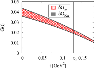
Figure 1: G(t) with the uncertainties $\delta\mathrm{G}_{as}$ and $\delta\mathrm{G}_{K\pi}$ added in quadrature.

One observes that in the whole physical region of the $K^{L}_{\mu 3}$ decay the function $\mathrm{G(t)}$ does not exceed $20\%$ of the expected value of $\mathrm{lnC}$. The uncertainty $\delta\mathrm{G_{as}}$ which clearly dominates could be further reduced using a somewhat model dependent multi channel Omnes-Mushkelishvili construction extending the description of the scalar form factor to higher energies. Such a construction has been presented in Ref. [32] and in principle, it allows to infer the phase of the form factor above the elastic region. We have used this phase to check, that in the low-energy region of interest the model of Ref. [32] reproduces our function $\mathrm{G(t)}$ within errors.
For practical purposes we give a simple parametrization of $\mathrm{G(t)}$ in the physical region $m_{\mu}^{2}<t<t_{0}=(m_{K^{0}}-m_{\pi^{+}})^{2}$. Denoting $x=t/t_{0}$, the true function $\mathrm{G(t)}$ is to a very good accuracy reproduced by

$$\mathrm{G_{P}(t)}=xD+(1-x)d+x(1-x)k\leavevmode\nobreak\ ,$$ (23)

where $d=\mathrm{G}(0)$, $D=\mathrm{G(t_{0})}$ and $k$ is obtained from the constraint $\mathrm{G}(\Delta_{K\pi})=0$. The central values of the three parameters $d$, $D$ and $k$ are collected in Table 1 together with the corresponding errors arising from $\delta\mathrm{G}_{K\pi}$ and from $\delta\mathrm{G_{as}}$. The uncertainties shown in Table 1 are correlated as implied by Eqs. (21) and (22). For the central values of Table 1, the deviation of the polynomial approximation $\mathrm{G_{P}(t)}$ from the exact function G(t) does not exceed $1\%$ of G(t) in the whole physical region.

	Central value	$\delta\mathrm{G}_{as}$	$\delta\mathrm{G}_{K\pi}$
$d$	0.0398	0.0036	0.002
$D$	0.0209	0.0016	0.001
$k$	0.0045	0.0001

Table 1: Coefficients arising in the parametrization $\mathrm{G_{P}}$ with their uncertainties.

It should be stressed that an accurate determination of $\mathrm{lnC}$ using the dispersive representation Eq. (16) in the fit of measured distributions only allows to infer from Eq. (15) the combination

$$\Delta\epsilon=2(\epsilon_{S}-\epsilon_{NS})+\tilde{\Delta}_{CT}$$ (24)

of the Callan Treiman discrepancy $\tilde{\Delta}_{CT}$ as defined by Eq. (8) ($\tilde{\Delta}_{CT}=\Delta_{CT}/B_{exp}$) and the RHCs parameter $\epsilon_{S}-\epsilon_{NS}$. In order to isolate the latter, the theoretical input of the former is required. Including isospin breaking effects at the order ${\cal O}(p^{4},(m_{d}-m_{u})p^{2},e^{2}p^{2})$ and varying the input parameters ($R=\frac{m_{s}-\hat{m}}{m_{d}-m_{u}}$, $F_{\pi}$, $L_{9}$ and $L_{5}$) one obtains from the $\chi PT$ formula displayed in [34] $\Delta_{CT}$ in the range $-0.005\div-0.001$ to be compared with the Gasser-Leutwyler estimate [21] given previously. This numerical result is somewhat sensitive to the use of the Gell-Mann-Okubo formula for the $\eta$ mass at that order, indicating a possible im-

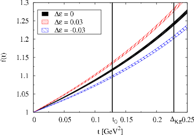
Figure 2: The scalar form factor $f(t)$. Central curve: $\Delta\epsilon=0$, top curve: $\Delta\epsilon=0.03$, bottom curve: $\Delta\epsilon=-0.03$ with uncertainties from experimental branching ratios and from G(t) added in quadrature.

portance of the ${\cal O}(p^{6})$ contribution. The precision of this estimate could be improved once the two loop $\chi PT$ analysis of $K_{l3}$ form factors [16] will be completed determining the relevant ${\cal O}(p^{6})$ LECs. At present our result suggests $\tilde{\Delta}_{CT}$ an order of magnitude smaller than the possible values of $\Delta\epsilon$ indicated by recent data [1] (see section V).

In Fig. 2 we show the sensitivity of the normalized scalar form factor $f(t)$ to the parameter $\Delta\epsilon$, Eq. (24). The central curve shows the form factor $f(t)$ for $\Delta\epsilon=0$ as given by the dispersive representation Eq. (16) with the use of Eq. (15). The error arising from experimental branching ratios as well as the error $\delta\mathrm{G(t)}$ are superposed to the curve. The two extreme curves with their error bars represent the form factor in the cases $\Delta\epsilon=\pm 0.03$. Once more it is seen that the uncertainties are much smaller than the possible signal of RHCs.
We add a comment on the parametrization of the form factor $\hat{f}_{+}(t)$. At present, it seems difficult to construct a one-parametrical representation of $\hat{f}_{+}(t)$ which would be as accurate as the representation Eq. (16) of the scalar form factor $f$. The reason is that the inelasticity in the $K\pi$-scattering P-wave sets in at lower energies and furthermore, the experimental information on $K^{+}\pi^{+}\to K^{+}\pi^{+}$ P-wave is still missing. Under these circumstances, it seems preferable to continue using the simple two-parametrical representation [1]:

$$\hat{f}_{+}(t)=\frac{f_{+}^{K^{0}\pi^{-}}(t)}{f_{+}^{K^{0}\pi^{-}}(0)}=1+\lambda_{+}\frac{t}{m_{\pi}^{2}}+\frac{1}{2}\lambda^{\prime}_{+}\Bigl{(}\frac{t}{m_{\pi}^{2}}\Bigr{)}^{2}\leavevmode\nobreak\ ,$$ (25)

keeping in mind the probable relevance of the curvature term.

V. In existing fixed target experiments, one usually does not know the energy of the decaying $K_{L}$ and for this reason it is difficult to reconstruct the $t=(p_{K}-p_{\pi})^{2}$ distribution. The parametrization of the two form factors then becomes of prime importance. On the other hand, it is difficult to justify a given parametrization experimentally otherwise than ad hoc, through a $\chi^{2}$ of a global fit of measured decay distributions. Under these circumstances the interpretation of the measured parameters may become somewhat ambiguous. Keeping in mind that in actual experiments it may be difficult to determine more than one parameter in the scalar form factor $f(t)$ [1], either the linear parametrization

$$f(t)=1+\lambda\frac{t}{m_{\pi}^{2}}\leavevmode\nobreak\ ,$$ (26)

or the ”pole parametrization”

$$f(t)=\frac{M^{2}_{S}}{M^{2}_{S}-t}\leavevmode\nobreak\ ,$$ (27)

is being standardly used, with a value for $\lambda$ and/or $M_{S}$ as the outcome of the fit. To the extent that the formulae Eq. (26) or (27) do not correctly account for the curvature of the form factor in the physical region, it may be questionable whether the parameters $\lambda$ or $M_{S}$ measured in this way can indeed be interpreted as $m_{\pi}^{2}f^{\prime}(0)$ or as the position of a pole, respectively.
One of the obvious advantages of the dispersive representation Eq. (16) is that it describes both the linear slope $\lambda$ and the curvature in terms of the single parameter $\mathrm{lnC}$. Consider the Taylor expansion

$$f(t)=1+\lambda\frac{t}{m_{\pi}^{2}}+\frac{1}{2}\lambda^{\prime}(\frac{t}{m_{\pi}^{2}})^{2}+\ldots\leavevmode\nobreak\ .$$ (28)

The linear slope is

$$\lambda=\frac{m_{\pi}^{2}}{\Delta_{K\pi}}(\mathrm{lnC}-d)\leavevmode\nobreak\ ,$$ (29)

whereas the curvature reads

$$\lambda^{\prime}=\lambda^{2}-2\frac{m_{\pi}^{4}}{\Delta_{K\pi}}G^{\prime}(0)=\lambda^{2}+(4.16\pm 0.50)\times 10^{-4}$$ (30)

It is worth stressing that the lower bound $\lambda^{\prime}>\lambda^{2}$ is a general consequence of the positive sign of the phase $\delta_{K\pi}(s)$ at low energies. Furthermore, even the pole parametrization Eq. (27) for which $\lambda^{\prime}=2\lambda^{2}$ underestimates the curvature Eq. (30) given by the dispersive theory, unless $\lambda>0.020$ or $M_{S}<1$ GeV (which seems excluded by the KTeV results [1]). Note that truncating the Taylor expansion Eq. (28) at the quadratic order and using Eq. (30) for the curvature, represents by itself an excellent approximation in the physical region though not as good as Eq. (23).
Let us illustrate and quantify the difficulty one encounters when the KTeV result $\lambda_{exp}=0.01372\pm 0.00131$ [1] based on the linear parametrization of $f(t)$ and a quadratic parametrization of $f_{+}(t)$ is converted into an information on the RHCs. For this purpose we define the effective (t-dependent) slope

$$f(t)=1+\lambda_{eff}(t)\frac{t}{m_{\pi}^{2}}.$$ (31)

Since $f(t)$ is convex, $\lambda_{eff}(t)$ grows as $t$ increases from $0$ to $t_{0}$ . For every fixed $0\leq t\leq t_{0}$, $\lambda_{eff}$ is a function of $\mathrm{lnC}$ or, using Eq. (15), of the variable $\Delta\epsilon=2(\epsilon_{S}-\epsilon_{NS})+\tilde{\Delta}_{CT}$ which we want to constrain. For the extreme cases $t=0$ and $t=t_{0}$, these two curves are displayed in Fig. 3 together with the corresponding uncertainties. The problem is that nothing in the KTeV analysis tells whether the measured value $\lambda_{exp}$ should be interpreted as $\lambda_{eff}(0)$, $\lambda_{eff}(t_{0})$ or $\lambda_{eff}$ at any other point of the physical region. Following whether $\lambda_{exp}$ is identified either with the slope at $t=0$ or with the slope at $t=t_{0}$, one obtains respectively:

$$\lambda_{exp}=\lambda_{eff}(0)\Rightarrow\mathrm{lnC}=0.2005\pm 0.0153\pm 0.0040\leavevmode\nobreak\ ,$$ (32)

$$\lambda_{exp}=\lambda_{eff}(t_{0})\Rightarrow\mathrm{lnC}=0.1748\pm 0.0141\pm 0.0019\leavevmode\nobreak\ ,$$ (33)

In both cases, the first error stems from the KTeV error bars whereas the second quoted error originates from $\delta\mathrm{G(t)}$. The difference of these two extreme values of $\mathrm{lnC}$ reflects the ambiguity arising because the theoretically inappropriate linear parametrization has been used in the analysis of KTeV data. It has little to do with a genuine experimental or theoretical error. Awaiting an unambiguous measurement of $\mathrm{lnC}$ based on a faithfull parametrization of $f(t)$, we use an admittedly arbitrary definition of the central value of $\mathrm{lnC}$ identifying $\lambda_{exp}$ with the average effective slope $\bar{\lambda}_{eff}$:

$$\lambda_{exp}=\bar{\lambda}_{eff}=\frac{1}{t_{0}}\int_{0}^{t_{0}}dt\,\lambda_{eff}(t)\leavevmode\nobreak\ .$$ (34)

This gives

$$\mathrm{lnC}=0.188\pm 0.015\pm 0.003\pm 0.013\leavevmode\nobreak\ ,$$ (35)

where to the experimental error and theoretical error arising from $\delta\mathrm{G}$ we have added the uncertainty due to the inadequate parametrization of the form factor used in the analysis (the half of the difference between Eq. (32) and Eq. (33)). This last ”parametrization uncertainty” is not a gaussian error and it should not be added in quadrature. Yet it is almost as big as the genuine experimental error. The corresponding constraint on the parameter $\Delta\epsilon$ and on the RHCs is obtained comparing Eq. (35) with Eq. (15):

$$\Delta\epsilon=2(\epsilon_{S}-\epsilon_{NS})+\tilde{\Delta}_{CT}=-0.029\pm 0.015\pm 0.003\pm 0.013\leavevmode\nobreak\ .$$ (36)

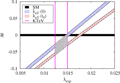
Figure 3: Impact of KTeV data on RHCs. Horizontal line: SM, $\Delta\epsilon=\tilde{\Delta}_{CT}=\pm\leavevmode\nobreak\ 0.0028$, vertical lines: KTeV measurements of $\lambda_{0}$. Top stripped curve: $\lambda_{exp}=\lambda_{eff}(0)$ and bottom stripped curve: $\lambda_{exp}=\lambda_{eff}(t_{0})$ with uncertainties from branching ratios and from G(t) added in quadrature.

Thanks to the ”parametrization uncertainty” this result for $\Delta\epsilon$ is still compatible with zero, i.e. with the SM. (Recall that $\tilde{\Delta}_{CT}$ is expected of the order $\sim 2.8\leavevmode\nobreak\ 10^{-3}$ [21]). This rough result $\Delta\epsilon=-0.03\pm 0.03$ summarized in Fig. 3 is rather robust. In particular, it does not depend on the detailed prescription Eq. (34) of defining the central value of $\mathrm{lnC}$.

VI We finally come to the charged K-decay mode $K^{+}\to\pi^{0}\mu\nu$. In full analogy to the neutral Kaon mode (cf Eq. 8), we can define the corresponding Callan-Treiman discrepancy $\Delta^{K^{+}}_{CT}$. Using the E865 result [33] for $|f_{+}^{K^{+}\pi^{0}}(0){\cal V}_{eff}^{us}|$, we obtain:

$$\mathrm{lnC}^{K^{+}}=0.1798\pm 0.0105+\tilde{\Delta}_{CT}^{K^{+}}+2(\epsilon_{S}-\epsilon_{NS})+{\cal O}(\epsilon^{2})\leavevmode\nobreak\ ,$$ (37)

where $\tilde{\Delta}_{CT}^{K^{+}}=\Delta_{CT}^{K^{+}}/B_{exp}^{K^{+}}=\Delta_{CT}^{K^{+}}/1.20$. Note that the experimental uncertainty is about 3 times larger than in the neutral case, Eq. (15), and of the same order of magnitude as the expected effect of RHCs. Furthermore, the effect of isospin breaking on $\Delta_{CT}^{K^{+}}$ due to $m_{d}-m_{u}$ is amplified by small denominators arising from $\pi^{0}$-$\eta$ mixing. Evaluating $\Delta_{CT}^{K^{+}}$ at order ${\cal O}(p^{4},(m_{d}-m_{u})p^{2},e^{2}p^{2})$ within $\chi PT$ using the results of [34] we find an increase of a few percent. (A similar increase is already observed in the decay rate [35].) Varying the parameters as described for $K^{0}$, one gets: $0.02<\Delta_{CT}^{K^{+}}<0.05$. Thus compared with the neutral case Eq. (15), the decrease of the first number on the RHS of Eq. (37) (reflecting the decrease of $B_{exp}^{K^{+}}$) could be compensated by a larger value of $\Delta_{CT}^{K^{+}}$. It thus seems that the analysis of RHCs from the $K^{+}_{\mu 3}$ experiment [36] is more involved requiring among other things a better knowledge of the isospin breaking parameter $\epsilon^{(2)}=\frac{\sqrt{3}}{4}\frac{1}{R}$.

VII. a) In this paper, we have constructed an accurate low-energy dispersive representation of the scalar $K\pi$ form factor in terms of a single parameter $C=f(\Delta_{K\pi})$ which describes both its slope and its curvature. The result, in a form ready to be used in a $K^{L}_{\mu 3}$ decay analysis is presented in Eqs. (16), (23) and in Table 1. Alternatively, an even simpler but somewhat less accurate quadratic parametrization could be used provided the slope and curvature are related by Eq. (30).
b) We have shown that a measurement of lnC at the 0.01 level would provide a significant test of direct electroweak couplings of right-handed quarks to the standard $W$-boson. So far no such a test is available beyond the specific framework of left-right symmetric extensions of the Standard Model.
c) Using the recent KTeV data [1] we have shown that the linear parametrization of the scalar form factor leads to a ”parametrization uncertainty” in lnC comparable with the actual experimental error $\pm 0.015$. This loss of information can be avoided taking into account the curvature of the form factor as suggested in this paper.
d) In parallel, matching the measured parameter $C=f(\Delta_{K\pi})$, the slope and the curvature of the scalar form factor with the two-loop $\chi PT$ [16] would help the assessment of the CKM element $V_{L}^{us}$.

Acknowledgements: We thank A. Ceccucci, H. Leutwyler, B. Moussallam and J.A. Oller for their interest, suggestions and help. Work supported in part by the EU RTN contract HPRN-CT-2002-00311 (EURIDICE) and by the EU I3HP contract RII3-CT-2004-506078.

References

- [1] T. Alexopoulos et al. [KTeV Collaboration], Phys. Rev. D 70 (2004) 092007 [arXiv:hep-ex/0406003].
- [2] A. Winhart for the NA48 collaboration, talk given at HEP2005, Lisboa, Portugal
-
[3]
R. N. Mohapatra and J. C. Pati,
Phys. Rev. D 11 (1975) 2558;
G. Senjanovic and R. N. Mohapatra, Phys. Rev. D 12 (1975) 1502. -
[4]
R. N. Mohapatra,
PRINT-84-0012 (MARYLAND)
Based on Lecture given at NATO Summer School on Particle Physics, Munich, West Germany, Sep 5-16, 1983;
P. Langacker and S. Uma Sankar, Phys. Rev. D 40 (1989) 1569. -
[5]
F. del Aguila, M. Perez-Victoria and J. Santiago,
JHEP 0009 (2000) 011
[arXiv:hep-ph/0007316];
P. Langacker and D. London, Phys. Rev. D 39 (1989) 266. - [6] W. Buchmüller and D. Wyler, Nucl. Phys. B 268 (1986) 621.
-
[7]
J. Hirn and J. Stern,
Eur. Phys. J. C 34 (2004) 447
[arXiv:hep-ph/0401032];
J. Hirn and J. Stern, Phys. Rev. D 73 (2006) 056001, [arXiv:hep-ph/0504277]. -
[8]
C. Csaki, C. Grojean, J. Hubisz, Y. Shirman and J. Terning,
Phys. Rev. D 70 (2004) 015012
[arXiv:hep-ph/0310355];
R. Sekhar Chivukula, E. H. Simmons, H. J. He, M. Kurachi and M. Tanabashi, Phys. Rev. D 72 (2005) 015008 [arXiv:hep-ph/0504114]. -
[9]
M. A. B. Beg, R. V. Budny, R. N. Mohapatra and A. Sirlin,
Phys. Rev. Lett. 38 (1977) 1252
[Erratum-ibid. 39 (1977) 54];
B. R. Holstein and S. B. Treiman, Phys. Rev. D 16 (1977) 2369;
W. Fetscher and H. J. Gerber, in [10] p657-705;
P. Herczeg, in [10] p786-837. - [10] P. Langacker,(ed.), Precision tests of the standard electroweak model, Singapore: World Scientific (1995).
- [11] J. Hirn and J. Stern, JHEP 0409 (2004) 058 [arXiv:hep-ph/0403017]
-
[12]
C. P. Burgess, S. Godfrey, H. Konig, D. London and I. Maksymyk,
Phys. Rev. D 49 (1994) 6115
[arXiv:hep-ph/9312291];
R. Barbieri and A. Strumia, Phys. Lett. B 462 (1999) 144 [arXiv:hep-ph/9905281];
Z. Han and W. Skiba, Phys. Rev. D 71 (2005) 075009 [arXiv:hep-ph/0412166]. -
[13]
H. Abramowicz et al.,
Z. Phys. C 12 (1982) 225;
S. R. Mishra et al., Phys. Rev. Lett. 68 (1992) 3499. -
[14]
J. F. Donoghue and B. R. Holstein,
Phys. Lett. B 113 (1982) 382;
I. I. Y. Bigi and J. M. Frere, Phys. Lett. B 110 (1982) 255. - [15] D. Becirevic et al., Nucl. Phys. B 705 (2005) 339 [arXiv:hep-ph/0403217].
- [16] J. Bijnens and P. Talavera, Nucl. Phys. B 669 (2003) 341 [arXiv:hep-ph/0303103].
- [17] V. Cirigliano, G. Ecker, M. Eidemuller, R. Kaiser, A. Pich and J. Portoles, JHEP 0504 (2005) 006 [arXiv:hep-ph/0503108].
- [18] G. D’Ambrosio, G. F. Giudice, G. Isidori and A. Strumia, Nucl. Phys. B 645 (2002) 155 [arXiv:hep-ph/0207036];
- [19] G. Beall, M. Bander and A. Soni, Phys. Rev. Lett. 48 (1982) 848.
- [20] R. F. Dashen and M. Weinstein, Phys. Rev. Lett. 22 (1969) 1337.
- [21] J. Gasser and H. Leutwyler, Nucl. Phys. B 250 (1985) 517.
- [22] W. J. Marciano, Phys. Rev. Lett. 93 (2004) 231803 [arXiv:hep-ph/0402299].
- [23] T. Alexopoulos et al. [KTeV Collaboration], Phys. Rev. Lett. 93 (2004) 181802 [arXiv:hep-ex/0406001].
- [24] A. Lai et al. [NA48 Collaboration], Phys. Lett. B 602 (2004) 41 [arXiv:hep-ex/0410059].
- [25] F. Ambrosino et al. [KLOE Collaboration], Phys. Lett. B 632 (2006) 43 [arXiv:hep-ex/0508027].
- [26] J. C. Hardy and I. S. Towner, Phys. Rev. C 71 (2005) 055501 [arXiv:nucl-th/0412056].
- [27] W. J. Marciano and A. Sirlin, Phys. Rev. Lett. 96 (2006) 032002 [arXiv:hep-ph/0510099].
- [28] V. Bernard, M. Oertel, E. Passemar, and J. Stern, in preparation.
- [29] G. P. Lepage and S. J. Brodsky, Phys. Lett. B 87 (1979) 359.
-
[30]
P. Estabrooks, R. K. Carnegie, A. D. Martin, W. M. Dunwoodie, T. A. Lasinski and D. W. G. Leith,
Nucl. Phys. B 133 (1978) 490;
D. Aston et al., Nucl. Phys. B 296 (1988) 493. - [31] P. Buettiker, S. Descotes-Genon and B. Moussallam, Eur. Phys. J. C 33 (2004) 409 [arXiv:hep-ph/0310283].
- [32] M. Jamin, J. A. Oller and A. Pich, Nucl. Phys. B 622 (2002) 279 [arXiv:hep-ph/0110193].
- [33] A. Sher et al., Phys. Rev. Lett. 91 (2003) 261802 [arXiv:hep-ex/0305042].
- [34] V. Cirigliano, M. Knecht, H. Neufeld, H. Rupertsberger and P. Talavera, Eur. Phys. J. C 23 (2002) 121 [arXiv:hep-ph/0110153].
- [35] V. Cirigliano, H. Neufeld and H. Pichl, Eur. Phys. J. C 35 (2004) 53 [arXiv:hep-ph/0401173].
- [36] O. P. Yushchenko et al., Phys. Lett. B 581 (2004) 31 [arXiv:hep-ex/0312004].