Abstract

We evaluate the LHC discovery potential for a light Higgs boson in $t\bar{t}H\,(\to\ell\nu b\bar{b}b\bar{b}jj)$ production, within the Standard Model and if a new $Q=2/3$ quark singlet $T$ with a moderate mass exists. In the latter case, $T$ pair production with decays $T\bar{T}\to W^{+}b\,H\bar{t}/Ht\,W^{-}\bar{b}\to W^{+}bW^{-}\bar{b}H$ provides an important additional source of Higgs bosons giving the same experimental signature, and other decay modes $T\bar{T}\to Ht\,H\bar{t}\to W^{+}b\,W^{-}\bar{b}$ $HH$, $T\bar{T}\to Zt\,H\bar{t}/Ht\,Z\bar{t}\to W^{+}bW^{-}\bar{b}HZ$ further enhance this signal. Both analyses are carried out with particle-level simulations of signals and backgrounds, including $t\bar{t}$ plus $n=0,\dots,5$ jets which constitute the main background by far. Our estimate for SM Higgs discovery in $t\bar{t}H$ production, $0.4\sigma$ significance for $M_{H}=115$ GeV and an integrated luminosity of 30 fb^-1, is similar to the most recent ones by CMS which also include the full $t\bar{t}nj$ background. We show that, if a quark singlet with a mass $m_{T}=500$ GeV exists, the luminosity required for Higgs discovery in this final state is reduced by more than two orders of magnitude, and $5\sigma$ significance can be achieved already with 8 fb^-1. This new Higgs signal will not be seen unless we look for it: with this aim, a new specific final state reconstruction method is presented. Finally, we consider the sensitivity to search for $Q=2/3$ singlets. The combination of these three decay modes allows to discover a 500 GeV quark with 7 fb^-1 of luminosity.

1 Introduction

The discovery of the Higgs boson is one of the main goals of the Large Hadron Collider (LHC). Our present understanding of electroweak symmetry breaking in the Standard Model (SM) relies on the existence of at least one of such scalar particles [1], whose mass is however not predicted. Direct searches at LEP have placed the limit $M_{H}>114.4$ GeV on the mass of a SM-like Higgs, with a 95% confidence level (CL) [2]. Actually, data taken from the ALEPH collaboration showed an excess of events over the SM background consistent with a 115 GeV Higgs boson, but these results were not confirmed by the other LEP collaborations. There is some theoretical prejudice leading us to believe in the existence of a Higgs boson not much heavier than this direct bound. Precision electroweak data seem to indicate its existence, with a best-fit value of $M_{H}=91^{+45}_{-32}$ GeV for its mass [3] if the SM is assumed. On the other hand, the Higgs boson must be lighter than around 1 TeV if the SM is required to remain perturbative up to the unification scale [4].

There is a vast Higgs search program at LHC, including various production processes and the decay channels relevant in each mass range [5, 6]. Most analyses focus on the search of a SM-like Higgs boson. For masses $M_{H}\lesssim 130$ GeV the decay $H\to b\bar{b}$ dominates, with a branching fraction around $0.7$. However, the most important production process $gg\to H$ is not visible in this channel due to the enormous QCD background. One has then to fall back either on rare decay modes, production processes in association with extra particles, or both. One example is the production together with a $t\bar{t}$ pair, with $H\to b\bar{b}$ and semileptonic decay of $t$, $\bar{t}$. Further examples are $gg\to H$ followed by $H\to\gamma\gamma$ (which has a branching ratio around 0.2%), or associate production $t\bar{t}H$, $WH$, $ZH$ with $H\to\gamma\gamma$. Simulations performed by the ATLAS collaboration [7, 8] estimated that $t\bar{t}H$ with $H\to b\bar{b}$ allows to reach $5\sigma$ significance for a 120 GeV Higgs boson with an integrated luminosity of 100 fb^-1, while very recent results from CMS [9], with a more realistic background calculation, considerably lower these expectations: even in the ideal case of no systematic uncertainties, $5\sigma$ significance could only be possible with $\sim 180$ fb^-1 (combining several decay channels of the $t\bar{t}$ pair). Hence, discovery of $t\bar{t}H$, with $H\to b\bar{b}$, seems unfeasible. However, the combination of $H$, $t\bar{t}H$, $WH$ and $ZH$ production, with $H\to\gamma\gamma$, is expected to give $5\sigma$ already with 60 fb^-1, providing also a relatively precise measurement of the Higgs mass. Vector boson fusion (VBF) processes $qq\to q^{\prime}q^{\prime}H$, with $H\to W^{+}W^{-}\to\ell^{+}\nu\ell^{{}^{\prime}-}\nu$, provide a similar sensitivity [10].

For larger Higgs masses the prospects are better. For $130\lesssim M_{H}\lesssim 2M_{W}$, $gg\to H$ production with decay $H\to ZZ^{*}\to\ell^{+}\ell^{-}\ell^{{}^{\prime}+}\ell^{{}^{\prime}-}$ provides a very clean experimental signature of four charged leptons. A Higgs particle with $M_{H}=130$ GeV may be detected in this channel with 15 fb^-1, and for $M_{H}=150$ GeV the luminosity required is reduced to 3 fb^-1. VBF processes are also interesting in this mass range, allowing to discover the Higgs with 12.9 fb^-1 for $M_{H}=130$ GeV and 3.5 fb^-1 for $M_{H}=150$ GeV [10]. For slightly larger masses, $2M_{W}\lesssim M_{H}<2M_{Z}$, the $H\to ZZ$ mode gets very suppressed due to the appearance of the on-shell decay $H\to W^{+}W^{-}$. Two signals are interesting in this range: $gg\to H$, with $W^{+}W^{-}\to\ell^{+}\nu\ell^{{}^{\prime}-}\nu$, giving $5\sigma$ significance for a luminosity around 4 fb^-1 [11], and again VBF processes, with leptonic or semileptonic decays of the $W$ pair, which improve this result giving the same sensitivity for 2 fb^-1. For masses larger than $2M_{Z}$, the mode $H\to ZZ$ is possible with both $Z$ bosons on their mass shell. This channel alone can signal the existence of a Higgs boson with a luminosity ranging from 2.6 fb^-1 for $M_{H}=200$ GeV to 32 fb^-1 for $M_{H}=600$ GeV [12]. Larger masses up to approximately 1 TeV can be probed combining different channels.

In SM extensions these production mechanisms can be enhanced or suppressed, and new ones may appear. In this work we analyse in detail a new production mechanism [14], possible when the top quark mixes with a new $Q=2/3$ singlet. Such particles appear in Little Higgs models [15], extra-dimensions [16], and grand unified theories [17]. They can be produced in pairs at LHC, through standard QCD interactions, with a large cross section for moderate masses of few hundreds of GeV. Their decays are determined by their mixing with SM quarks, which (by theoretical considerations and experimental constraints) is expected to be largest with the third generation. In particular, their decays to $Ht$ occur with a branching ratio close to 25% for $M_{H}\ll m_{T}$. This possibility would be especially welcome, since it increases the observability of a Higgs boson in the mass region $M_{H}\lesssim 130$ GeV where its detection is more difficult. For definiteness, we will assume $M_{H}=115$ GeV, though the results are rather insensitive to the Higgs mass, as long as the main decay channel is $H\to b\bar{b}$. The largest cross section corresponds to

$$gg,q\bar{q}\to T\bar{T}\to W^{+}b\,H\bar{t}/Ht\,W^{-}\bar{b}\to W^{+}b\,W^{-}\bar{b}\,H\,,$$ (1)

with semileptonic decay of the $W$ pair and $H\to b\bar{b}$. It gives the same experimental signature $\ell\nu b\bar{b}b\bar{b}jj$ as SM $t\bar{t}H$ production but the kinematics is rather different. Two further processes contribute to the Higgs signal,

$$gg,q\bar{q}\to T\bar{T}\to Ht\,H\bar{t}\to W^{+}b\,W^{-}\bar{b}\,HH\,,$$

$$gg,q\bar{q}\to T\bar{T}\to Zt\,H\bar{t}/Ht\,Z\bar{t}\to W^{+}b\,W^{-}\bar{b}\,HZ\,,$$ (2)

yielding the same final state, or the same state plus two jets, when the extra Higgs and $Z$ boson decay $H\to b\bar{b},c\bar{c}$, $Z\to q\bar{q},\nu\bar{\nu}$. In this work we compare the discovery potential in this final state within the SM (in which case the only signal is $t\bar{t}H$) and with a new singlet $T$, assuming for its mass a reference value $m_{T}=500$ GeV. It has been shown that such a particle could be seen at LHC in a short time, through its decays $T\bar{T}\to W^{+}bW^{-}\bar{b}$ [18]. Experimental search in the $\ell\nu b\bar{b}b\bar{b}jj$ final state would improve the statistical significance of the $T$ signal and, what is perhaps even more important, it would allow a prompt discovery of the Higgs boson.

We remark that, in contrast to what happens with a fourth sequential generation [20], a quark singlet contributes very little to $gg\to H$ in general, due to its tiny Yukawa coupling obtained by mixing with the top quark. The amplitudes for $gg\to H$ mediated by $T$ and top quarks, relative to the SM one (involving the top quark only), can be written as

$$\frac{A(T)}{A(t)_{\text{SM}}} = \frac{y_{HTT}}{y_{Htt}|_{\text{SM}}}\left[\frac{I(m_{T}^{2}/M_{H}^{2})}{I(m_{t}^{2}/M_{H}^{2})}\right]=\frac{m_{T}X_{TT}}{m_{t}}\left[\frac{I(m_{T}^{2}/M_{H}^{2})}{I(m_{t}^{2}/M_{H}^{2})}\right]\,,$$

$$\frac{A(t)}{A(t)_{\text{SM}}} = \frac{y_{Htt}}{y_{Htt}|_{\text{SM}}}=X_{tt}$$ (3)

being $X_{TT}$, $X_{tt}$ mixing factors (see next section for details) and $I$ a loop function. The ratio in brackets is very close to unity for a light Higgs, and takes the value $0.977$ for $M_{H}=115$ GeV, $m_{T}=500$ GeV. With typical values $X_{TT}\simeq 0.04$, $X_{tt}\simeq 0.96$ for the mixing factors, for $m_{T}=500$ GeV the $T$ amplitude is about 9 times smaller than the SM one, and the top quark contribution is reduced by a factor $0.96$. We also note that in particular SM extensions including $Q=2/3$ singlets other processes and/or channels may be enhanced or suppressed. An interesting example takes place in Little Higgs models, where the $gg\to H$ cross section may be suppressed but the branching ratio for $H\to\gamma\gamma$ can increase in some regions of parameter space, due to the extra contribution of the new fermions to the effective $H\gamma\gamma$ vertex [13]. We finally note that in models with one (or more) $Q=-1/3$ singlet $B$ there are large Higgs signals from $B\bar{B}$ production and decay $B\to Hb$, giving different final states from the ones studied here [14].

2 Summary of the model

SM extensions with vector-like quarks under $\text{SU}(2)_{L}$ have been introduced before, and their phenomenology has been extensively explored [21, 22, 23, 24]. Here we will briefly recall the main features of a SM extension with a $Q=2/3$ quark singlet, summarising the most relevant points for this work. The addition of two $\mathrm{SU}(2)_{L}$ singlet fields $T^{0}_{L,R}$ to the quark spectrum modifies the weak and scalar interactions involving $Q=2/3$ quarks, but does not affect strong and electromagnetic interactions. (We denote weak eigenstates with a zero superscript, to distinguish them from mass eigenstates which do not bear superscripts.) Thus, the new $Q=2/3$ mass eigenstate $T$ can be produced in pairs in $pp$ collisions via QCD interactions like the top quark. The production cross section, plotted in Fig. 1, decreases with $m_{T}$ but is sizeable for $T$ masses of several hundreds of GeV. For our evaluations we will take $m_{T}=500$ GeV, well above the present limit from Tevatron $m_{T}\geq 258$ GeV at 95% CL [25].

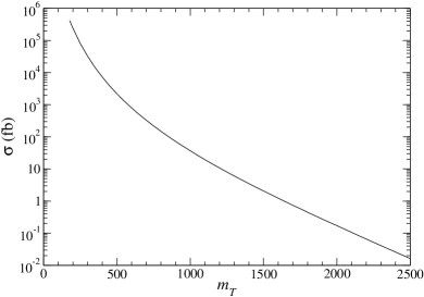
Figure 1: Total production cross section for $gg,q\bar{q}\to T\bar{T}$ for different $T$ masses.

The decay of the new quark takes place through electroweak and scalar interactions. Using standard notation, these interactions read

$$\mathcal{L}_{W} = -\frac{g}{\sqrt{2}}\left[\bar{u}\gamma^{\mu}VP_{L}d\;W_{\mu}^{+}+\bar{d}\gamma^{\mu}V^{\dagger}P_{L}u\;W_{\mu}^{-}\right]\,,$$

$$\mathcal{L}_{Z} = -\frac{g}{2c_{W}}\bar{u}\gamma^{\mu}\left[XP_{L}-\frac{4}{3}s_{W}^{2}\leavevmode\hbox{\small 1\kern-3.8pt\normalsize 1}_{4\times 4}\right]u\;Z_{\mu}\,,$$

$$\mathcal{L}_{H} = \frac{g}{2M_{W}}\,\bar{u}\left[\mathcal{M}^{u}XP_{L}+X\mathcal{M}^{u}P_{R}\right]u\;H\,,$$ (4)

where $u=(u,c,t,T)$, $d=(d,s,b)$ and $P_{R,L}=(1\pm\gamma_{5})/2$. The extended Cabibbo-Kobayashi-Maskawa (CKM) matrix $V$ is of dimension $4\times 3$, $X=VV^{\dagger}$ is a non-diagonal $4\times 4$ matrix and $\mathcal{M}^{u}$ is the $4\times 4$ diagonal up-type quark mass matrix. The new mass eigenstate $T$ is expected to couple mostly with third generation quarks $t$, $b$, because $T_{L}^{0}$, $T_{R}^{0}$ preferably mix with $t_{L}^{0}$, $t_{R}^{0}$, respectively, due to the large top quark mass. $V_{Tb}$ is mainly constrained by the contribution of the new quark to the $\mathrm{T}$ parameter [24]. For $m_{T}=500$ GeV, the most recent value $\mathrm{T}=-0.03\pm 0.09$ [26] implies $|V_{Tb}|\leq 0.17$ with a 95% CL. Mixing of $T_{L}^{0}$ with $u_{L}^{0}$, $c_{L}^{0}$, especially with the latter, is very constrained by parity violation experiments and the measurement of $R_{c}$ and $A_{\mathrm{FB}}^{0,c}$ at LEP, respectively [22, 27], implying small $X_{uT}$, $X_{cT}$. The charged current couplings with $d,s$ must be small as well, $|V_{Td}|,|V_{ts}|\sim 0.05$, because otherwise the new quark would give large loop contributions to kaon and $B$ physics observables [24]. Therefore, $|V_{Td}|,|V_{Ts}|\ll|V_{Tb}|$ and $|X_{uT}|,|X_{cT}|\ll|X_{tT}|$. The couplings of the $t,T$ quarks can be expressed in terms of the charged current coupling $V_{Tb}$,

$$|V_{tb}|^{2} \simeq 1-|V_{Tb}|^{2}\,,$$

$$X_{tt} \simeq 1-|V_{Tb}|^{2}\,,$$

$$X_{TT} \simeq |V_{Tb}|^{2}\,,$$

$$|X_{tT}|^{2} \simeq |V_{Tb}|^{2}(1-|V_{Tb}|^{2})\,.$$ (5)

As it has been mentioned above, the $T\bar{T}$ cross section is independent of $V_{Tb}$ and, as we will see below, branching ratios are independent too. The only place where this mixing appears is the total $T$ width, which is much smaller than the experimental resolution for the $T$ mass. Thus, $V_{Tb}$ has no influence at all in our results. For definiteness, we have taken for our evaluations a coupling $V_{Tb}=0.2$. This value is slightly above the most recent 95% limit from the $\mathrm{T}$ parameter (and compatible with the previous one, $|V_{Tb}|\leq 0.26$). For this coupling, the Yukawa coupling of the top quark is $y_{Htt}=(m_{t}/2M_{W})\,X_{tt}$, reduced by a factor 0.96 with respect to its SM value, and the Yukawa of the new quark is very small, $y_{HTT}=(m_{T}/2M_{W})\,X_{TT}$ with $X_{TT}=0.04$. The relevant decays of the new quark are $T\to W^{+}b,\,Zt,\,Ht$, with partial widths

$$\Gamma(T\to W^{+}b) =\frac{\alpha}{16\,s_{W}^{2}}|V_{Tb}|^{2}\frac{m_{T}^{3}}{M_{W}^{2}}\left[1-3\frac{M_{W}^{4}}{m_{T}^{4}}+2\frac{M_{W}^{6}}{m_{T}^{6}}\right]\,,$$

$$\Gamma(T\to Zt) =\frac{\alpha}{32s_{W}^{2}c_{W}^{2}}|X_{tT}|^{2}\frac{m_{T}}{M_{Z}^{2}}\lambda(m_{T},m_{t},M_{Z})^{1/2}$$

$$\times\left[1+\frac{M_{Z}^{2}}{m_{T}^{2}}-2\frac{m_{t}^{2}}{m_{T}^{2}}-2\frac{M_{Z}^{4}}{m_{T}^{4}}+\frac{m_{t}^{4}}{m_{T}^{4}}+\frac{M_{Z}^{2}m_{t}^{2}}{m_{T}^{4}}\right]\,,$$

$$\Gamma(T\to Ht) =\frac{\alpha}{32s_{W}^{2}}|X_{tT}|^{2}\frac{m_{T}}{M_{W}^{2}}\lambda(m_{T},m_{t},M_{H})^{1/2}$$

$$\times\left[1+6\frac{m_{t}^{2}}{m_{T}^{2}}-\frac{M_{H}^{2}}{m_{T}^{2}}+\frac{m_{t}^{4}}{m_{T}^{4}}-\frac{m_{t}^{2}M_{H}^{2}}{m_{T}^{4}}\right]\,,$$ (6)

with

$$\lambda(m_{T},m_{t},M)\equiv(m_{T}^{4}+m_{t}^{4}+M^{4}-2m_{T}^{2}m_{t}^{2}-2m_{T}^{2}M^{2}-2m_{t}^{2}M^{2})$$ (7)

a kinematical function. The two couplings $V_{Tb}$, $X_{tT}$ involved in the decays are approximately equal (see Eq. (5)). Since the three partial widths are proportional to $|V_{Tb}|^{2}$, the branching ratios only depend on $m_{T}$ and $M_{H}$. They are plotted in Fig. 2 for a fixed value $M_{H}=115$ GeV. For $m_{T}=500$ GeV, we have $\mathrm{Br}(T\to W^{+}b)=0.503$, $\mathrm{Br}(T\to Zt)=0.166$, $\mathrm{Br}(T\to Ht)=0.331$. (The total $T$ width is $\Gamma_{T}=3.115$ for $V_{Tb}=0.2$.) Decays $T\to Zt\to\ell^{+}\ell^{-}W^{+}b$, $\ell=e,\mu$ give a cleaner final state than $T\to W^{+}b$, but with a branching ratio 10 times smaller. The channel $T\to W^{+}b$ ($\bar{T}\to W^{-}\bar{b}$) gives the best discovery potential for the new quark in single $T$ [28] as well as in $T\bar{T}$ production [18]. The remaining decay $T\to Ht$ constitutes a copious source of Higgs bosons for moderate $T$ masses, for which the $T\bar{T}$ production cross section is large. We point out that in the minimal SM extension where only one $Q=2/3$ singlet is introduced these branching ratios are independent of the mixing, and the new quark (provided it is not decoupled) always decays $T\to Ht$ if $m_{T}>m_{t}+M_{H}$. In models with extra interactions, decays to $W^{\prime}$, $Z^{\prime}$ bosons may occur, if kinematically allowed. If additional scalars exist, mixing with the lightest one $H$ might also be suppressed, if this Higgs is not SM-like.

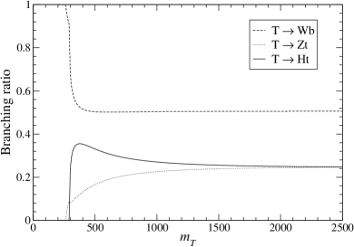
Figure 2: Branching ratios for $T\to W^{+}b$, $T\to Zt$, $T\to Ht$, for different $T$ masses.

3 Signal and background simulation

Many SM and some new physics processes give or mimic the experimental signature studied of a charged lepton, at least four $b$-tagged jets and two non-tagged jets, plus missing energy. The relevant processes are calculated with matrix-element-based Monte Carlo generators and fed into PYTHIA [29] to include initial and final state radiation (ISR, FSR) and pile-up, and perform hadronisation. The main background is constituted by $t\bar{t}+n$ jet production. It is calculated, with $n=0,\dots,5$, with ALPGEN [30], using the MLM prescription [31] to avoid double counting of jet radiation performed by PYTHIA. ALPGEN is also used to calculate the production of $W$ and $Z$ bosons plus six jets, or a $b\bar{b}\,/\,c\bar{c}$ pair and four jets. New Monte Carlo generators are developed for $T\bar{T}$, $t\bar{t}H$, $t\bar{t}b\bar{b}$ and $t\bar{t}c\bar{c}$ (through QCD and electroweak (EW) interactions) and $Wb\bar{b}b\bar{b}$ production, plus other processes obtained replacing the top quarks by heavy $T$ quarks. These generators use the full resonant tree-level matrix elements for the production and decay processes, namely

$$gg,q\bar{q} \to T\bar{T}\to W^{+}b\,H\bar{t}/Ht\,W^{-}\bar{b}\to W^{+}bW^{-}\bar{b}H\to f_{1}\bar{f}_{1}^{\prime}b\bar{f}_{2}f_{2}^{\prime}\bar{b}\;b\bar{b}/c\bar{c}\,,$$

$$gg,q\bar{q} \to T\bar{T}\to Ht\,H\bar{t}\to W^{+}bW^{-}\bar{b}HH\to f_{1}\bar{f}_{1}^{\prime}b\bar{f}_{2}f_{2}^{\prime}\bar{b}\;b\bar{b}/c\bar{c}\;b\bar{b}/c\bar{c}\,,$$

$$gg,q\bar{q} \to T\bar{T}\to Zt\,H\bar{t}/Ht\,Z\bar{t}\to W^{+}bW^{-}\bar{b}HZ\to f_{1}\bar{f}_{1}^{\prime}b\bar{f}_{2}f_{2}^{\prime}\bar{b}\;b\bar{b}/c\bar{c}\;q\bar{q}/\nu\bar{\nu}\,,$$

$$gg,q\bar{q} \to T\bar{T}\to W^{+}b\,Z\bar{t}/Zt\,W^{-}\bar{b}\to W^{+}bW^{-}\bar{b}Z\to f_{1}\bar{f}_{1}^{\prime}b\bar{f}_{2}f_{2}^{\prime}\bar{b}\;b\bar{b}/c\bar{c}\,,$$

$$gg,q\bar{q} \to T\bar{T}\to Zt\,Z\bar{t}\to W^{+}bW^{-}\bar{b}ZZ\to f_{1}\bar{f}_{1}^{\prime}b\bar{f}_{2}f_{2}^{\prime}\bar{b}\;q\bar{q}/\nu\bar{\nu}\;q\bar{q}/\nu\bar{\nu}\,,$$

$$gg,q\bar{q} \to t\bar{t}H\to W^{+}bW^{-}\bar{b}H\to f_{1}\bar{f}_{1}^{\prime}b\bar{f}_{2}f_{2}^{\prime}\bar{b}\;b\bar{b}/c\bar{c}\,,$$

$$gg,q\bar{q} \to t\bar{t}b\bar{b}\to W^{+}bW^{-}\bar{b}b\bar{b}\to f_{1}\bar{f}_{1}^{\prime}b\bar{f}_{2}f_{2}^{\prime}\bar{b}\,b\bar{b}\,,$$

$$gg,q\bar{q} \to t\bar{t}c\bar{c}\to W^{+}bW^{-}\bar{b}c\bar{c}\to f_{1}\bar{f}_{1}^{\prime}b\bar{f}_{2}f_{2}^{\prime}\bar{b}\,c\bar{c}\,,$$

$$q\bar{q}^{\prime} \to W^{\pm}b\bar{b}b\bar{b}\to f_{1}\bar{f}_{1}^{\prime}b\bar{b}b\bar{b}\,.$$ (8)

Matrix elements are calculated with HELAS [35], partly using MadGraph [36]. All finite width and spin effects are thus automatically taken into account. The colour flow information necessary for PYTHIA is obtained following the same method as in AcerMC [37], i.e. we randomly select the colour flow among the possible ones on an event-by-event basis, computing the probabilities of such a configuration from the matrix element (taking into account the diagrams contributing to such configuration). Integration in phase space is done with VEGAS [38], modified following Ref. [37]. These generators (except $Wb\bar{b}b\bar{b}$) have been checked against ALPGEN using the same parameters, structure functions and factorisation scales, obtaining very good agreement. For our evaluations we take $m_{t}=175$ GeV, $m_{b}=4.8$ GeV, $m_{c}=1.5$ GeV (neglected in $W$ decays), $\alpha(M_{Z})=1/128.878$, $s_{W}^{2}(M_{Z})=0.23113$, $\alpha_{s}(M_{Z})=0.127$ and run the coupling constants up to the the scale of the heavy ($t$ or $T$) quark. Structure functions CTEQ5L [39] are used, with $Q^{2}=\hat{s}$ the square of the partonic centre of mass energy. (For ALPGEN processes we select $Q^{2}=M_{t,W,Z}^{2}+p_{t_{t,W,Z}}^{2}$.) Several representative total cross sections obtained (without decay branching ratios nor phase space cuts) can be found in Table 1, for comparison with other generators. The total cross sections for $t\bar{t}c\bar{c}$, $t\bar{t}nj$ with $n\geq 1$ and $W/Z+$ jets are numerically unstable due to collinear singularities and not shown. This is not a problem for event generation, since suitable kinematical cuts at the generator level (discussed below) can be applied to stabilise the cross sections.

Process	$\sigma_{\text{tot}}$
$t\bar{t}$ (ALPGEN)	489 pb
$T\bar{T}$	2.14 pb
$t\bar{t}H$	508 fb
$t\bar{t}b\bar{b}$	8.65 pb
$t\bar{t}b\bar{b}$ EW	773 fb
$Wb\bar{b}b\bar{b}$	303.4 fb

Table 1: Total cross sections for several processes studied.

In our analysis we consider semileptonic decays of the $W^{+}W^{-}$ pairs, and leptonic decays in the production of $W/Z\,+$ jets. The main contributions come from $\ell=e,\mu$, but decays to $\tau$ leptons are included as well. Phase space cuts are applied at the generator level in some processes to reduce statistical fluctuations and improve the unweighting efficiency. The cuts applied are

$$t\bar{t}nj |\eta^{j}|\leq 2.5\;,~{}p_{t}^{j}\geq 20~{}\text{GeV}\;,~{}\Delta R^{jj}\geq 0.4$$

$$t\bar{t}b\bar{b},t\bar{t}c\bar{c},Wb\bar{b}b\bar{b} |\eta^{b,c}|\leq 2.5\;,~{}p_{t}^{b,c}\geq 15~{}\text{GeV}$$

$$Wb\bar{b}jjjj,Wc\bar{c}jjjj,Wjjjjjj |\eta^{\ell,b,j}|\leq 2.5\;,~{}p_{t}^{\ell}\geq 6~{}\text{GeV}\;,~{}p_{t}^{b,j}\geq 15~{}\text{GeV}\;,$$

$$\Delta R^{jj,bb}\geq 0.4\;,~{}\Delta R^{\ell j,\ell b}\geq 0.4$$

$$Zb\bar{b}jjjj,Zc\bar{c}jjjj,Wjjjjjj |\eta^{b,j}|\leq 2.5\;,~{}p_{t}^{\ell,\text{max}}\geq 6~{}\text{GeV}\;,~{}p_{t}^{b,j}\geq 15~{}\text{GeV}\;,$$

$$\Delta R^{jj,bb}\geq 0.4\,,$$ (9)

where $\eta$ is the pseudorapidity, $p_{t}$ the transverse momentum and $\Delta R\equiv\sqrt{(\Delta\eta)^{2}+(\Delta\phi)^{2}}$ the lego-plot distance. The cross sections after decay, including generator cuts, can be read in Table 2 for $\ell=e,\mu$. The $T\bar{T}$ processes in Eqs. (8) will from now on be denoted according to the decay mode as $T\bar{T}\,(WH)$, $T\bar{T}\,(HH)$, $T\bar{T}\,(ZH)$, $T\bar{T}\,(WZ)$ and $T\bar{T}\,(ZZ)$. Sum over charge conjugate decays is always understood.

Process	$\sigma$	$\varepsilon$		Process	$\sigma$	$\varepsilon$
$T\bar{T}\,(WH)$	173.6 fb	6.3%		$t\bar{t}b\bar{b}$	564.9 fb	4.7%
$T\bar{T}\,(HH)$	44.38 fb	19.3%		$t\bar{t}c\bar{c}$	630.5 fb	0.65%
$T\bar{T}\,(ZH)$	50.0 fb	8.5%		$t\bar{t}b\bar{b}$ EW	60.31 fb	4.8%
$T\bar{T}\,(WZ)$	29.03 fb	4.5%		$t\bar{t}c\bar{c}$ EW	17.12 fb	0.72%
$T\bar{T}\,(ZZ)$	14.07 fb	2.8%		$Wjjjjjj$	69.85 pb	$\sim 7.4\times 10^{-6}$
$T\bar{T}b\bar{b}$	1.054 fb	5.3%		$Wb\bar{b}jjjj$	2.825 pb	0.12%
$t\bar{t}H$	118.7 fb	4.7%		$Wc\bar{c}jjjj$	3.279 pb	$\sim 0.015$%
$t\bar{t}$	143.2 pb	0.034%		$Wb\bar{b}b\bar{b}$	2.587 fb	$\sim 3.4$ %
$t\bar{t}j$	142.7 pb	0.055%		$Zjjjjjj$	10.48 pb	$\sim 3.9\times 10^{-6}$
$t\bar{t}2j$	95.9 pb	0.085%		$Zb\bar{b}jjjj$	722.5 fb	0.090%
$t\bar{t}3j$	54.0 pb	0.12%		$Zc\bar{c}jjjj$	738.5 fb	$\sim 0.013$%
$t\bar{t}4j$	27.4 pb	0.15%
$t\bar{t}5j$	12.8 pb	0.19%

Table 2: Cross section at the generator level and efficiency $\varepsilon$ for signal and background processes in the decay channels with $\ell=e,\mu$. The corresponding cross sections for final states with tau leptons are approximately one half, with efficiencies $20-30$ times smaller.

The generated events are passed through PYTHIA 6.403 as external processes to include ISR, FSR, pile-up and perform hadronisation. We use the standard PYTHIA settings except for $b$ fragmentation, in which we use the Peterson parameterisation with $\epsilon_{b}=-0.0035$ [40]. For pile-up we take 4.6 events in average, corresponding to a luminosity of $2\times 10^{33}\;\text{cm}^{-2}\;\text{s}^{-1}$. Tau leptons in the final state are decayed using TAUOLA [32] and PHOTOS [33]. A fast detector simulation ATLFAST 2.60 [34], with standard settings, is used for the modelling of the ATLAS detector. We reconstruct jets using a cone algorithm with $\Delta R=0.4$. This cone size has proved to be the most adequate for top physics studies [41], providing very good agreement between fast and full simulations for reconstructed quantities [42]. We do not apply trigger inefficiencies and assume a perfect charged lepton identification. The package ATLFASTB is used to recalibrate jet energies and perform $b$ tagging, for which we select a 60% efficiency at the low luminosity run, with nominal rejection factors of 93 for light jets and 6.7 for charm, and $p_{t}$-dependent corrections. These efficiencies are in agreement with those obtained from full simulations [43], and comparable to the ones expected at CMS [44].

The hadronised events are required to fulfill these two criteria: (a) the presence of one (and only one) isolated charged lepton, which must have transverse momentum $p_{t}\geq 25$ GeV (for electrons), $p_{t}\geq 20$ GeV (for muons) and $|\eta|\leq 2.5$; (b) at least six jets with $p_{t}\geq 20$ GeV, $|\eta|\leq 2.5$, with at least four $b$ tags and two untagged jets. The charged leptons provide a trigger for the events [45]. Signal and background efficiencies after these requirements are shown in Table 2. We notice the higher acceptance for the $T\bar{T}\,(HH)$ process, with six $b$ quarks in the final state when both Higgs bosons decay to $b\bar{b}$, and for $T\bar{T}\,(ZH)$, where sometimes two $b$ quarks are produced in the $Z$ decay. We also point out the growing efficiency of the $t\bar{t}nj$ processes with increasing multiplicity.

Finally, we must note that our calculation of the $Wb\bar{b}b\bar{b}jj$ background, with $Wb\bar{b}b\bar{b}$ production at the generator level and extra jet radiation performed by PYTHIA, must be regarded as an estimate. The reason is that in $Wb\bar{b}b\bar{b}$ only $q\bar{q}^{\prime}$ scattering processes are involved, while gluon fusion contributes to $Wb\bar{b}b\bar{b}jj$. At any rate, this background turns out to be completely negligible. $Zb\bar{b}b\bar{b}$ production has an even smaller cross section and we have not included it in our calculations. We have investigated $t\bar{t}b\bar{b}b\bar{b}$ production with ALPGEN, which might be important if five or more $b$ tags are required. The cross section (with the same cuts used before) is of 0.54 fb. Assuming a similar detection efficiency as for $t\bar{t}b\bar{b}$, the requirement of five tagged jets reduces the cross section to one event for 30 fb^-1 (and 0.3 events with 6 $b$ tags). One may also think about $T\bar{T}H$ production, with $T\bar{T}\to W^{+}bW^{-}\bar{b}$, also contributing to the final state studied. This process is irrelevant due to the small Yukawa coupling of the $T$ quark.

4 Higgs boson discovery

We simulate events for an integrated luminosity of 30 fb^-1, which can be collected in three years at the low luminosity phase. For some background processes the number of events simulated corresponds to the cross section obtained from the generator scaled by a $k$ factor, to take into account higher order contributions with extra jets. (This $k$ factor accounting for higher multiplicity processes must not be confused with a $K$ factor to take radiative corrections into account.) For the main background, $t\bar{t}nj$ production, higher order processes are explicitly calculated, and $k$ factors are not included except for $N=5$, where we set $k=1.46$ to account for $t\bar{t}+6$ jets. For $t\bar{t}b\bar{b}$ and $t\bar{t}c\bar{c}$, the $k$ factor is estimated from the $t\bar{t}nj$ cross sections as $k=[\sigma(t\bar{t}2j)+\dots+\sigma(t\bar{t}6j)]/\sigma(t\bar{t}2j)=2.05$. For $W/Z$ plus jets we use the approximate prescription in Ref. [18], which gives $k=2-3$. For all signals we conservatively set $k=1$. The reason for this will be explained later. The number of events generated for each process can be read in Table 3. In the sums, the first term corresponds to final states with $\ell=e,\mu$ and the second one to $\ell=\tau$, but in the following all lepton channels will be summed. A subtlety in the analysis is that when the singlet $T$ is introduced the $Htt$, $Wtb$ and $Ztt$ couplings of the top quark are modified. This affects electroweak $t\bar{t}b\bar{b}$ and $t\bar{t}c\bar{c}$ production in a non-trivial way, and different samples (taking into account the corrections to the couplings) must be generated and simulated. $t\bar{t}H$ production is modified as well, with the Yukawa coupling of the top quark reduced by a factor $X_{tt}<1$. In our case, we have assumed a large mixing $V_{Tb}=0.2$, for which $|V_{tb}|=0.98$ and $X_{tt}=0.96$. These processes are indicated with a “$(T)$” in Table 3, where we can observe that the effect of mixing is negligible for $t\bar{t}b\bar{b}$ and $t\bar{t}c\bar{c}$. A second issue to keep in mind is that when studying the new physics signals associated to the $T$ quark we must distinguish the cases where the Higgs boson is present or not (if not, the branching ratios for $T\to W^{+}b$ and $T\to Zt$ are larger). The latter are denoted with a “$H\!\!\!\!\!\!\!\not\,\,\,\,\,$”.

	$N_{0}$	$N$			$N_{0}$	$N$
$T\bar{T}\,(WH)$	$5200^{*}+2600^{*}$	$329.8+9.2$		$t\bar{t}b\bar{b}$	$34700+17400$	$1648+35$
$T\bar{T}\,(HH)$	$1330^{*}+665^{*}$	$256.5+6.2$		$t\bar{t}c\bar{c}$	$38800+19300$	$253+8$
$T\bar{T}\,(ZH)$	$1500^{*}+750^{*}$	$127.4+3.1$		$t\bar{t}b\bar{b}$ EW	$3710^{*}+1850^{*}$	$178.1+3.2$
$T\bar{T}\,(WZ)$	$871^{*}+436^{*}$	$39.5+0.7$		$t\bar{t}b\bar{b}$ EW ($T$)	$3420^{*}+1710^{*}$	$170.7+2.9$
$T\bar{T}\,(WZ;H\!\!\!\!\!\!\!\not\,\,\,\,\,)$	$1950^{*}+975^{*}$	$87.7+2.3$		$t\bar{t}c\bar{c}$ EW	$1050^{*}+525^{*}$	$7.6+0.0$
$T\bar{T}\,(ZZ)$	$422^{*}+211^{*}$	$11.9+0.2$		$t\bar{t}c\bar{c}$ EW ($T$)	$980^{*}+490^{*}$	$6.3+0.1$
$T\bar{T}\,(ZZ;H\!\!\!\!\!\!\!\not\,\,\,\,\,)$	$939^{*}+470^{*}$	$27.3+0.4$		$Wjjjjjj$	$5270000+2640000$	$39+0$
$T\bar{T}b\bar{b}$	$31.6^{*}+15.4^{*}$	$1.7+0.0$		$Wb\bar{b}jjjj$	$168000+83900$	$208+4$
$T\bar{T}b\bar{b}\;(H\!\!\!\!\!\!\!\not\,\,\,\,\,)$	$70.8^{*}+34.6^{*}$	$4.1+0.1$		$Wc\bar{c}jjjj$	$195000+97400$	$29+1$
$t\bar{t}H$	$3560^{*}+1780^{*}$	$166.0+4.3$		$Wb\bar{b}b\bar{b}$	$118+59$	$4+1$
$t\bar{t}H$ ($T$)	$3280^{*}+1640^{*}$	$152.9+3.8$		$Zjjjjjj$	$1020000+510000$	$4+0$
$t\bar{t}$	$4368000+2184000$	$1475+23$		$Zb\bar{b}jjjj$	$53600+26800$	$48+5$
$t\bar{t}j$	$4282000+2141000$	$2370+48$		$Zc\bar{c}jjjj$	$54800+27400$	$7+1$
$t\bar{t}2j$	$2878000+1439000$	$2443+42$
$t\bar{t}3j$	$1620000+810000$	$1900+48$
$t\bar{t}4j$	$822000+411000$	$1195+45$
$t\bar{t}5j$	$562000+281000$	$1067+19$

Table 3: For each process: number of events simulated $N_{0}$ and number of events passing the pre-selection criteria $N$. The first terms in the sums correspond to $\ell=e,\mu$, and the second ones to $\ell=\tau$. For some contributions (marked with an asterisk) we have simulated at least $10N_{0}$ events and rescaled the result to 30 fb^-1, so as to reduce statistical fluctuations.

The discovery potential for the Higgs boson crucially depends on systematic errors. The uncertainty in the background normalisation makes it difficult to detect the presence of a Higgs boson with a measurement of the total $\ell\nu bbbbjj$ cross section. Naively, from the data in Table 3 one could conclude that the statistical significance of the $t\bar{t}H$ signal, before applying any kinematical cut, is $S/\sqrt{B}=170.3/\sqrt{13158.9}=1.48\sigma$. However, this estimate does not include the systematic uncertainty in the SM background total cross section (i.e. the background normalisation). A detailed calculation of systematic uncertainties is beyond the scope of this work. They generally arise from two sources: (i) the theoretical uncertainty in cross sections, due to higher loop contributions and uncertainty in parton distribution functions, among others; (ii) the systematic uncertainty related to the experimental detection ($b$ tagging, jet energy scaling, etc.). The former can go up to 30–50% for $t\bar{t}nj$ with large $n$, but they are reducible with more accurate theoretical calculations and/or background measurements (understanding to what extent they are reduced probably requires real data). For the latter we assume a “reference” value of 20%, close to the value $\sim 26\%$ obtained in Ref. [9] with a detailed analysis for the CMS detector. We replace the estimator $\mathcal{S}_{0}\equiv S/\sqrt{B}$ by

$$\mathcal{S}_{20}\equiv S/\sqrt{B+(0.2B)^{2}}\,,$$ (10)

where $S$ is the excess of events over the expected background. Incorporating systematic uncertainties in the previous example, we obtain a much smaller (but more realistic) significance $\mathcal{S}_{20}=0.064\sigma$. We note that adding statistical and systematic uncertainties in quadrature is not the only way to incorporate systematics into the significance. Other possibilities exist, which are perhaps more correct from the statistical point of view, but we use this one for simplicity and in order to compare better with other studies.

In the following we perform two different analyses of signals and backgrounds. The first one is a “standard” analysis aiming to discover the Higgs boson in $t\bar{t}H$ production, in which we reconstruct the final state to distinguish this signal from the SM background. In case that a new quark $T$ exists, additional signal events will improve the Higgs discovery potential. The second analysis specifically looks for a Higgs boson produced in heavy quark decays, optimising the reconstruction for this signal.

4.1 Analysis I: $\boldsymbol{t\bar{t}H}$ reconstruction

The reconstruction of the $t\bar{t}H$ signal is not done sequentially, but rather all possible pairings for light and $b$ jets are tried, selecting the one which best resembles the kinematics of this process. We reconstruct the $W$ boson decaying hadronically (called “hadronic” $W$ boson) from a pair of untagged jets $j_{1}$ and $j_{2}$. For the leptonic $W$, the missing transverse momentum is assigned to the neutrino, and its longitudinal momentum and energy are found requiring that the invariant mass of the charged lepton and neutrino is the $W$ mass, $(p_{\ell}+p_{\nu})^{2}=M_{W}^{2}$. This equation gives two real solutions in most cases. In case there is no real solution (the discriminant of the quadratic equation is negative) we set it to zero to obtain a solution. This procedure gives reconstructed mass distributions almost indistinguishable from the ones obtained using the collinear approximation, i.e. setting $p_{\nu}^{z}=p_{\ell}^{z}$.

For each choice of $j_{1}$, $j_{2}$ and leptonic $W$ momentum, there are 12 possible assignments of the four $b$ jets to the two $W$ bosons, to form the two top quarks. (Around 9% of the signal events have five or more $b$ jets, in which case we select the four with the highest transverse momentum.) Among all possibilities, we select the one minimising the quantity

$$\Delta m^{2}=\frac{(m_{t}^{\mathrm{had}}-m_{t})^{2}}{S_{t}^{2}}+\frac{(m_{t}^{\mathrm{lep}}-m_{t})^{2}}{S_{t}^{2}}+\frac{(M_{W}^{\mathrm{had}}-M_{W})^{2}}{S_{W}^{2}}\,,$$ (11)

where $m_{t}^{\mathrm{had}}$, $m_{t}^{\mathrm{lep}}$ and $M_{W}^{\mathrm{had}}$ are the reconstructed masses of the hadronic and leptonic top quarks, and the hadronic $W$, respectively. $S_{t}$ and $S_{W}$ are fixed parameters corresponding to the widths of the reconstructed distributions, which are taken in this case to be equal, $S_{t}=S_{W}=10$ GeV. For the best combination, the two remaining (unpaired) $b$ jets are assumed to originate from the Higgs boson decay, whose momentum and invariant mass can then be reconstructed. Kinematical cuts are not applied at this level. The results are shown in Fig. 3. The reconstruction works very well for the $t\bar{t}H$ signal, with sharp peaks for the reconstructed masses $M_{W}^{\mathrm{had}}$, $m_{t}^{\mathrm{had}}$ and $m_{t}^{\mathrm{lep}}$, and the Higgs mass distribution mainly concentrated around the true value $M_{H}=115$ GeV. Since the SM background is dominated by $t\bar{t}nj$ production with two top quarks, the invariant masses of the hadronic $W$ and the top pair are very well reconstructed too. For the $T\bar{T}$ Higgs signal this reconstruction method is not adequate, and the reconstructed Higgs mass spreads over a wider range.

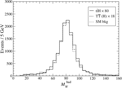
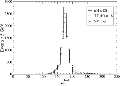
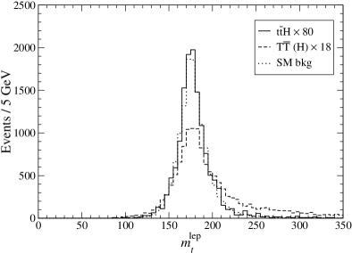
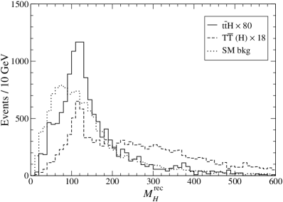
Figure 3: Analysis I: Reconstructed masses of the hadronic $W$, the hadronic and leptonic top quarks and the Higgs boson.

The signal significance can be improved by simply performing a kinematical cut on the Higgs reconstructed mass. Additionally, we perform a probabilistic analysis (see appendix A), involving the following variables:

• The light jet multiplicity $\mathcal{N}_{\text{jet}}$.

• The smallest invariant mass of a $bb$ pair $m_{bb}^{(1)}$ [7], among those involving the four jets with largest transverse momentum.

• The sum of the transverse momenta of the two top quarks, $p_{t}^{\text{had}}+p_{t}^{\text{lep}}$.

• Angular quantities characterising the topology of the event: the azimuthal angle and rapidity difference (i) between the two $b$ jets assigned to the Higgs, $\Delta\phi_{bb}$ and $\Delta\eta_{bb}$; (ii) between the Higgs and the closest (in $\Delta R$) top quark, $\Delta\phi_{Ht}$ and $\Delta\eta_{Ht}$; (iii) between the two top quarks, $\Delta\phi_{tt}$ and $\Delta\eta_{tt}$.

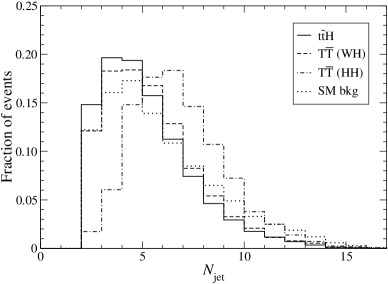
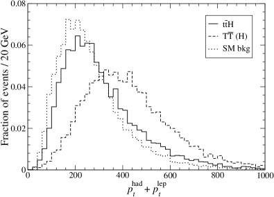
Figure 4: Analysis I: Normalised light jet multiplicity $\mathcal{N}_{\text{jet}}$ and variable $p_{t}^{\text{had}}+p_{t}^{\text{lep}}$ (see the text), used in the probabilistic analysis. The jet multiplicities of the two main $T\bar{T}$ Higgs signals are displayed separately for later convenience. The $p_{t}^{\text{had}}+p_{t}^{\text{lep}}$ distribution for the $T\bar{T}$ Higgs signals is shown for illustration, but not included in the probabilistic analysis as a separate event class.

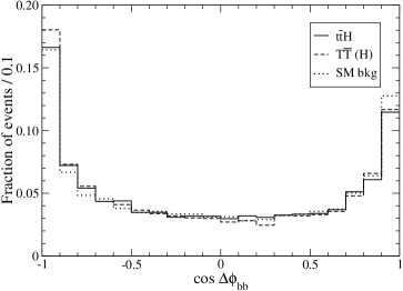
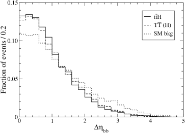
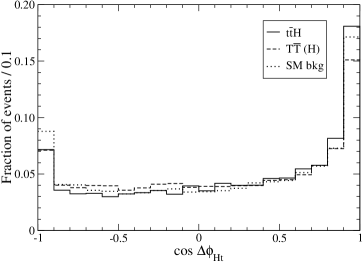
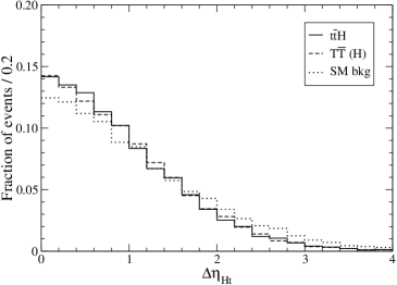
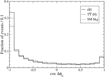
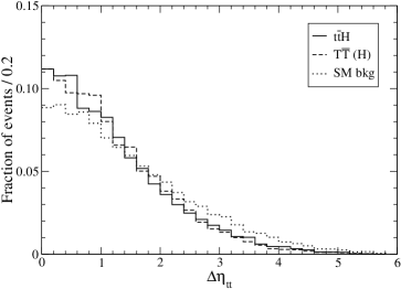
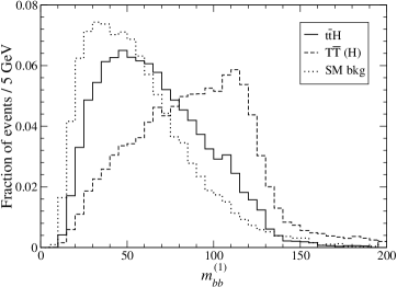
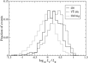
Figure 5: Analysis I: Normalised variables $\cos\Delta\phi_{bb}$, $\Delta\eta_{bb}$, $\cos\Delta\phi_{Ht}$, $\Delta\eta_{Ht}$, $\cos\Delta\phi_{tt}$, $\Delta\eta_{tt}$ and $m_{bb}^{(1)}$ (defined in the text), used in the probabilistic analysis. Log-likelihood function. The distributions for the $T\bar{T}$ Higgs signals are shown for illustration, but not included in the probabilistic analysis as a separate event class.

These variables, plotted in Figs. 4, 5 for the background and reference signal samples (with more statistics), are not suitable for kinematical cuts but help distinguish $t\bar{t}H$ production from the SM background. Additional variables can be considered, but we have found no improvement including them, and in some cases they reduce the discriminating power of the likelihood functions (for a discussion see the appendix). Using their distributions for $t\bar{t}H$ and the SM background we build signal and background likelihood functions $L_{S}$, $L_{B}$. The log-likelihood function $\log_{10}L_{S}/L_{B}$ is also plotted in Fig. 5. In the absence of systematic errors, the highest statistical significance $\mathcal{S}_{0}=S/\sqrt{B}$ would be achieved with relatively loose cuts on $L_{S}/L_{B}$. But when one considers systematic uncertainties, the highest significance $\mathcal{S}_{20}$ is found for more strict cuts, which reduce the background to few tens of events. For this purpose, we have found it very useful to employ a hybrid event selection method, in which we perform a simple cut on the Higgs reconstructed mass and include the rest of the relevant variables in the likelihood function. The kinematical cuts applied (not fine-tuned but close to the optimal values) are

$$\log_{10}L_{S}/L_{B}\geq 0.75\,,$$

$$100~{}\text{GeV}\leq M_{H}^{\mathrm{rec}}\leq 140~{}\text{GeV}\,.$$ (12)

The number of events corresponding to each process can be read in Table 4. We point out that the inclusion of the light jet multiplicity as a likelihood variable significantly reduces the $t\bar{t}nj$ background for larger $n$. $W/Z$ plus jets is essentially eliminated for high $L_{S}$ values, even without requiring explicitly a good $M_{W}^{\mathrm{had}}$, $m_{t}^{\mathrm{had}}$ and $m_{t}^{\mathrm{lep}}$ reconstruction. With these selection cuts a statistical significance $\mathcal{S}_{20}=0.39\sigma$ is found for 30 fb^-1. This sensitivity is much lower than in previous ATLAS analyses [7, 8] but similar to the most recent one by CMS, $\mathcal{S}_{20}=0.47\sigma$. However, it must be noted that the CMS analysis uses full detector simulation, including the electron and muon efficiencies not taken here into account. On the other hand, the next-to-leading order cross section for $t\bar{t}H$ is used in that analysis, which is 1.5 times larger than the one taken here.

	$N_{\text{cut}}$			$N_{\text{cut}}$			$N_{\text{cut}}$
$T\bar{T}\,(WH)$	5.1		$t\bar{t}$	0		$t\bar{t}b\bar{b}$ EW	0.4
$T\bar{T}\,(HH)$	3.5		$t\bar{t}j$	5		$t\bar{t}c\bar{c}$ EW	0.0
$T\bar{T}\,(ZH)$	1.8		$t\bar{t}2j$	6		$Wjjjjjj$	0
$T\bar{T}\,(WZ)$	0.4		$t\bar{t}3j$	4		$Wb\bar{b}jjjj$	0
$T\bar{T}\,(ZZ)$	0.0		$t\bar{t}4j$	2		$Wc\bar{c}jjjj$	0
$T\bar{T}b\bar{b}$	0.1		$t\bar{t}5j$	0		$Wb\bar{b}b\bar{b}$	0
$t\bar{t}H$	2.5		$t\bar{t}b\bar{b}$	4		$Zjjjjjj$	0
			$t\bar{t}c\bar{c}$	0		$Zb\bar{b}jjjj$	0
						$Zc\bar{c}jjjj$	0

Table 4: Analysis I: number of events $N_{\text{cut}}$ after the selection criteria in Eqs. (12).

We remark that the signal itself has additional higher order contributions $t\bar{t}Hnj$, with $n\geq 1$, which have not been included in the same way as $t\bar{t}nj$ because the implementation of the matching prescription is not yet available (and also for consistency with the calculation of $T\bar{T}$, in which only the lowest order $n=0$ can be generated). When higher order processes are included, there are two alternatives for the likelihood analysis: (i) keep using the $\mathcal{N}_{\text{jet}}$ distribution for $t\bar{t}H$ in Fig. 4, which suppresses $t\bar{t}nj$ but also $t\bar{t}Hnj$ for larger $n$; (ii) use a new $\mathcal{N}_{\text{jet}}$ distribution for $t\bar{t}Hnj$, which may improve the results. The first option can always be followed, and will of course lead to better results than the ones shown here (this is the reason why we have not included any $k$ factors in the signals). Thus, the results shown here are conservative. From the number of $t\bar{t}nj$ events in Table 4 we can estimate that the inclusion of higher $t\bar{t}Hnj$ processes would double the sensitivity at least. These comments also apply to the case in which $\mathcal{N}_{\text{jet}}$ is not included in the likelihood but a cut on this variable is performed (see the next section).

The new Higgs signals from $T\bar{T}$ decays enhance the observability of the Higgs boson. Despite the very different kinematics of this process, and the fact that the reconstruction is aimed at identifying $t\bar{t}H$ production, $T\bar{T}$ events are more signal- than background-like, as it can be observed in Figs. 4– 5. Hence, they are not very suppressed by the kinematical cuts, and enhance the Higgs sensitivity by a factor of 6, $\mathcal{S}_{20}=2.03\sigma$. This improvement is sufficient to have hints of the Higgs boson with a luminosity of 30 fb^-1. However, one can do much better with a dedicated reconstruction aiming to detect the new quark.

4.2 Analysis II: $\boldsymbol{T\bar{T}}$ reconstruction

The three different $T\bar{T}$ decay channels considered yield final states with four or six $b$ quarks, and lead to signal events with four, five and six or more $b$-tagged jets. (Due to mistags, the number of $b$ jets may be occasionally larger than the number of $b$ quarks at the partonic level.) The number of events corresponding to each decay channel and number of $b$ jets are collected in Table 5, including also the SM background.

	Total	4 tags	5 tags	$\geq 6$ tags
$T\bar{T}\,(WH)$	339.0	303.2	33.7	2.1
$T\bar{T}\,(HH)$	262.7	166.0	76.5	20.2
$T\bar{T}\,(ZH)$	130.5	97.9	27.3	5.3
Background	13158.9	12572.4	561.1	25.4

Table 5: Analysis II: Number of events (for 30 fb^-1) with four, five and six or more $b$ tags, for each of the signal processes and the SM background.

The discovery potential is higher if signal and background samples are separated according to their $b$ jet multiplicity. This is also convenient from the point of view of the signal reconstruction. The two main signal channels,

$$T\bar{T}\to W^{+}b\,H\bar{t}/Ht\,W^{-}\bar{b}\to W^{+}bW^{-}\bar{b}H\to f_{1}\bar{f}_{1}^{\prime}b\bar{f}_{2}f_{2}^{\prime}\bar{b}\;b\bar{b} (WH)\,,$$

$$T\bar{T}\to Ht\,H\bar{t}\to W^{+}bW^{-}\bar{b}HH\to f_{1}\bar{f}_{1}^{\prime}b\bar{f}_{2}f_{2}^{\prime}\bar{b}\;b\bar{b}\;b\bar{b} (HH)\,,$$ (13)

have four and six $b$ quarks in the final state, respectively, and different kinematics. Hence, for the reconstruction the events are classified as follows:

• Events with four $b$ tags are assigned to the $WH$ mode and reconstructed accordingly.

• Events with six or more $b$ tags are assigned to the $HH$ mode.

• Events with five tags are assumed to belong to the $HH$ mode as well if there are at least three non-$b$ jets (the sixth $b$ jet is taken to be one of the non-tagged ones). A small fraction $\simeq 5$% which only has two light jets is reconstructed as in the $WH$ mode.

This separation allows for a better reconstruction of $T\bar{T}\,(HH)$ events with five or more $b$ tags, which amount to 36.6% of this channel and have a much smaller background. The remaining $T\bar{T}\,(HH)$ events only have four tags, and they are reconstructed as in the $T\bar{T}\,(WH)$ channel. In both methods the heavy quark mass is not used in order to not bias the SM background towards this invariant mass value. The reconstruction is done by trying all possible pairings for light and $b$ jets, and selecting the one which best resembles the kinematics of the decay channel considered.

4.2.1 $4b$ final states

We reconstruct the hadronic $W$ boson from a pair of light jets $j_{1}$ and $j_{2}$, and the leptonic $W$ from the charged lepton and missing transverse momentum. With the $W$ momenta determined up to a twofold ambiguity, we identify the two $b$ quarks $b_{T}$ and $b_{t}$ coming from the decays $T\to Wb$, $t\to Wb$. There are 24 possibilities for the pairing, because: (i) the heavy quark decaying to $Wb$ (irrespectively of whether it is $T$ or $\bar{T}$) may have the $W$ boson decaying hadronically or leptonically; (ii) the quark $b_{T}$ may correspond to each one of the four $b$-tagged jets in the final state, and the three remaining ones are then produced in the cascade decay $T\to Ht\to b\bar{b}Wb$; (iii) the quark $b_{t}$ from the top decay can be any of the latter three. Among the 48 resulting possibilities (plus different choices of $j_{1}$ and $j_{2}$), we select the one minimising the quantity

$$\Delta m^{2}_{WH}=\frac{(m_{T}^{\mathrm{had}}-m_{T}^{\mathrm{lep}})^{2}}{S_{T}^{2}}+\frac{(m_{t}^{\mathrm{rec}}-m_{t})^{2}}{S_{t}^{2}}+\frac{(M_{W}^{\mathrm{had}}-M_{W})^{2}}{S_{W}^{2}}\,,$$ (14)

where $m_{t}^{\mathrm{rec}}$ corresponds to the intermediate top quark (which may decay hadronically or leptonically), and $m_{T}^{\mathrm{had}}$, $m_{T}^{\mathrm{lep}}$ are the reconstructed masses of the hadronic and leptonic $T$ quarks (independently of whether they decay to $Wb$ or $Ht$). $S_{T}$, $S_{t}$ and $S_{W}$ are taken as $S_{T}=100$ GeV, $S_{t}=20$ GeV and $S_{W}=10$ GeV. No cuts are applied at this level. For the best pairing, the two remaining $b$ jets not assigned to the $T$ and $t$ decays correspond to the Higgs boson. The reconstructed masses are shown in Fig. 6 for the sum of signal channels and the SM background.

We build signal and background likelihood functions using:

• The reconstructed masses $m_{T}^{\mathrm{had}}$, $m_{T}^{\mathrm{lep}}$.

• Variables characterising the high transverse momentum of the signal: the total transverse energy $H_{T}$, the missing energy $p_{t}\!\!\!\!\!\!\!\!\not\,\,\,\,\,\,$, the maximum and second maximum $p_{t}$ of the $b$ jets $p_{t}^{b,\mathrm{max}}$ and $p_{t}^{b,\mathrm{max2}}$, and the second maximum $p_{t}$ of the light jets $p_{t}^{j,\mathrm{max2}}$.

• The energy of the charged lepton in the heavy quark rest frame, $E_{\ell}^{*}$. This distribution has a long tail for $T\bar{T}\,(WH)$ signal events, not only because of the large $T$ mass but also due to spin effects [46].

• The smallest invariant mass of a $bb$ pair $m_{bb}^{(1)}$ and the second smallest one $m_{bb}^{(2)}$.

• Angular quantities characterising the topology of the event: the azimuthal angle and rapidity difference (i) between the two $b$ jets assigned to the Higgs, $\Delta\phi_{bb}$ and $\Delta\eta_{bb}$; (ii) between the Higgs and the reconstructed top quark, $\Delta\phi_{Ht}$ and $\Delta\eta_{Ht}$; (iii) between the Higgs and its parent $T$ quark, $\Delta\eta_{HT}$.

The distributions of these variables are presented in Figs. 7, 8. We remark again that the selection of variables is not arbitrary, and some variables not considered, e.g. the transverse momentum of the charged lepton or the maximum transverse momentum of the light jets, have not been included because they actually reduce the discriminating power with respect to the set of variables above. This surprising fact is due to the correlation among variables, and is further explained in the appendix. We distinguish three likelihood classes: the $T\bar{T}\,(WH)$ and $T\bar{T}\,(HH)$ signals and the background. The signal likelihood is defined as the sum of the likelihoods of the two signal classes, $L_{S}=L_{S_{1}}+L_{S_{2}}$. The logarithm of $L_{S}/L_{B}$ is plotted in Fig. 8. We observe that the $T\bar{T}\,(WH)$ distributions are in general more distinguishable from the background than the $T\bar{T}\,(HH)$ ones. This results in a cleaner separation between $T\bar{T}\,(WH)$ and the background.

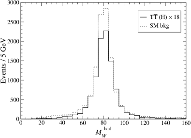
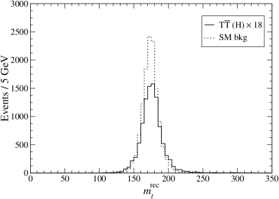
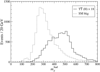
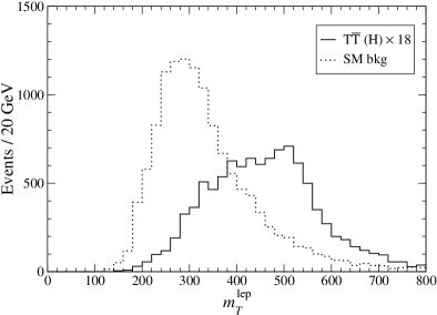
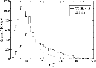
Figure 6: Analysis II ($4b$ final states): Reconstructed masses of the hadronic $W$, the top quark, the hadronic and leptonic heavy quarks and the Higgs boson, for the background and the sum of $T\bar{T}$ Higgs signals.

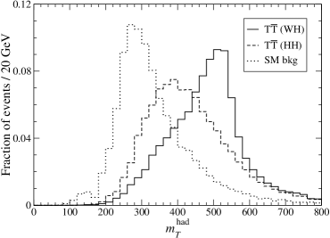
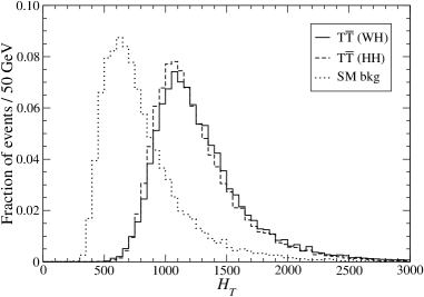
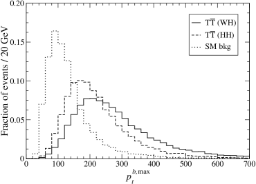
Figure 7: Analysis II ($4b$ final states): Normalised variables $m_{T}^{\mathrm{had}}$, $m_{T}^{\mathrm{lep}}$, $H_{T}$, $p_{t}\!\!\!\!\!\!\!\!\not\,\,\,\,\,\,$, $p_{t}^{b,\mathrm{max}}$, $p_{t}^{b,\mathrm{max2}}$, $p_{t}^{j,\mathrm{max2}}$ and $E_{\ell}^{*}$ (defined in the text), used in the likelihood analysis.

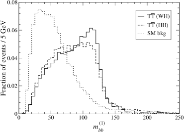
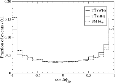
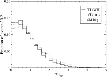
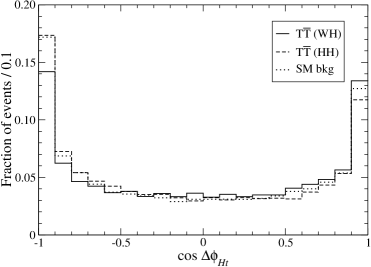
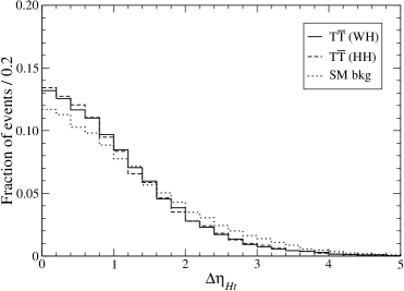
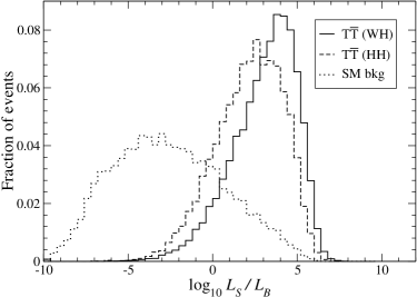
Figure 8: Analysis II ($4b$ final states): Normalised variables $m_{bb}^{(1)}$, $m_{bb}^{(2)}$, $\cos\Delta\phi_{bb}$, $\Delta\eta_{bb}$, $\cos\Delta\phi_{Ht}$, $\Delta\eta_{Ht}$ and $\Delta\eta_{HT}$ (defined in the text), used in the likelihood analysis. Log-likelihood function $\log_{10}L_{S}/L_{B}$.

For event selection we again use a hybrid method, with cuts on reconstructed masses, jet multiplicity and signal likelihood. The selection criteria are

$$\log_{10}L_{S}/L_{B}\geq 3.9\,,$$

$$\mathcal{N}_{\text{jet}}\leq 7\,,$$

$$100~{}\text{GeV}\leq M_{H}^{\mathrm{rec}}\leq 140~{}\text{GeV}\,,$$

$$350~{}\text{GeV}\leq m_{T}^{\mathrm{had}},m_{T}^{\mathrm{lep}}\leq 650~{}\text{GeV}\,.$$ (15)

The numbers of events after these cuts are collected in Table 6. The $t\bar{t}nj$ background with larger $n$ has larger transverse momenta and is less affected by the cut on likelihood, but it is suppressed by the cut on jet multiplicity. $W/Z$ plus jets is insignificant. We also note the smaller efficiency for the $T\bar{T}\,(HH)$ signal, expected since its likelihood function has a larger overlap with the background, see Fig. 8. Additionally, $T\bar{T}\,(HH)$ decays with four $b$-tagged jets have a larger light jet multiplicity, and are more affected by the requirement $\mathcal{N}_{\text{jet}}\leq 7$. The same comments made in the preceding subsection regarding the cut on $\mathcal{N}_{\text{jet}}$ and higher order signal processes apply here.

Before calculating the statistical significance of the Higgs signals from $T\bar{T}$ decays it is important to draw attention to the fact that, since neither the $T$ quark nor the Higgs boson have been discovered at present, there are two possible definitions for what we consider as signal and background. The first one would be to take as background just the SM processes in Table 3 (excluding $t\bar{t}H$), and for the signal $t\bar{t}H$, $T\bar{T}$ (in all decay modes) and $T\bar{T}b\bar{b}$. The second possibility is to take as background the SM processes (slightly modified by the presence of the heavy quark) plus $T\bar{T}\,(WZ,ZZ)$ and $T\bar{T}b\bar{b}$ in the absence of a Higgs boson (see Table 3). Signal plus background is then constituted by the SM processes, plus $T\bar{T}\,(WZ,ZZ)$ and $T\bar{T}b\bar{b}$ with a Higgs boson, and Higgs production processes $t\bar{t}H$ and $T\bar{T}\,(WH,HH,ZH)$. The “signal”, that is, the excess of events over the background, is thus $t\bar{t}H$ plus $T\bar{T}\,(WH,HH,ZH)$ plus the difference between $T\bar{T}\,(WZ,ZZ)$ and $T\bar{T}b\bar{b}$ with and without a Higgs boson, that is,

$$B = \text{SM bkg.}+T\bar{T}(WZ,ZZ;H\!\!\!\!\!\!\!\not\,\,\,\,\,)\,,$$

$$S = t\bar{t}H(T)+T\bar{T}(WH,HH,ZH)$$ (16)

$$+\left[T\bar{T}(WZ,ZZ)-T\bar{T}(WZ,ZZ;H\!\!\!\!\!\!\!\not\,\,\,\,\,)\right]+\Delta\,\text{SM bkg.}$$

The term in brackets is always negative, and the difference in SM background is negligible. Both conventions lead to appreciably different results, and we adopt the latter, which is more conservative. (This amounts to considering that the $T$ quark will have been discovered before the Higgs boson.) With this definition, the signal significance is $\mathcal{S}_{20}=6.43\sigma$, including a 20% systematic error.

	$N_{\text{cut}}$			$N_{\text{cut}}$			$N_{\text{cut}}$
$T\bar{T}\,(WH)$	36.2		$t\bar{t}$	1		$t\bar{t}c\bar{c}$ EW	0.0
$T\bar{T}\,(HH)$	5.4		$t\bar{t}j$	0		$t\bar{t}c\bar{c}$ EW ($T$)	0.0
$T\bar{T}\,(ZH)$	2.9		$t\bar{t}2j$	2		$Wjjjjjj$	0
$T\bar{T}\,(WZ)$	0.8		$t\bar{t}3j$	3		$Wb\bar{b}jjjj$	0
$T\bar{T}\,(WZ)$ ($H\!\!\!\!\!\!\!\not\,\,\,\,\,$)	2.1		$t\bar{t}4j$	8		$Wc\bar{c}jjjj$	0
$T\bar{T}\,(ZZ)$	0.0		$t\bar{t}5j$	2		$Wb\bar{b}b\bar{b}$	0
$T\bar{T}\,(ZZ)$ ($H\!\!\!\!\!\!\!\not\,\,\,\,\,$)	0.1		$t\bar{t}b\bar{b}$	3		$Zjjjjjj$	0
$T\bar{T}b\bar{b}$	0.0		$t\bar{t}c\bar{c}$	2		$Zb\bar{b}jjjj$	0
$T\bar{T}b\bar{b}$ ($H\!\!\!\!\!\!\!\not\,\,\,\,\,$)	0.1		$t\bar{t}b\bar{b}$ EW	0.5		$Zc\bar{c}jjjj$	0
$t\bar{t}H$ ($T$)	0.8		$t\bar{t}b\bar{b}$ EW ($T$)	0.3

Table 6: Analysis II ($4b$ final states): Number of events (for 30 fb^-1) after the kinematical cuts in Eq. (15).

4.2.2 $5b$ and $6b$ final states

Reconstructing the decay $T\bar{T}\to HtH\bar{t}\to HW^{+}bHW^{-}\bar{b}$ requires identifying six $b$ jets in the final state. In the case of five $b$ tags, a light jet $j_{b}$ (if there are at least three) may be assumed to come from a $b$ quark as well. The hadronic $W$ boson is reconstructed from a pair of untagged jets $j_{1}$ and $j_{2}$. The leptonic $W$ is reconstructed from the charged lepton momentum and missing energy. Each $W$ boson is associated to three $b$ jets to reconstruct the momenta of the $T$ quarks (there are 20 combinations). For each choice, there are $3\times 3$ possibilities to associate two $b$ jets to the hadronic and leptonic $W$, in order to reconstruct the two top quarks. The two remaining pairs of $b$ jets $(b_{1},b_{2})$, $(b_{3},b_{4})$ are assumed to come from the decays of the two Higgs bosons, with reconstructed masses $M_{H_{1}}^{\mathrm{rec}}=m_{b_{1}b_{2}}$ (associated to the hadronic top), $M_{H_{2}}^{\mathrm{rec}}=m_{b_{3}b_{4}}$ (associated to the leptonic one). Among the 360 resulting possibilities (plus different choices of $j_{1}$, $j_{2}$ and $j_{b}$), we select the one minimising the quantity

$$\Delta m^{2}_{HH} = \frac{(m_{T}^{\mathrm{had}}-m_{T}^{\mathrm{lep}})^{2}}{S_{T}^{2}}+\frac{(M_{H_{1}}^{\mathrm{rec}}-M_{H_{2}}^{\mathrm{rec}})^{2}}{S_{H}^{2}}+\frac{(m_{t}^{\mathrm{had}}-m_{t})^{2}}{S_{t}^{2}}+\frac{(m_{t}^{\mathrm{lep}}-m_{t})^{2}}{S_{t}^{2}}$$ (17)

$$+\frac{(M_{W}^{\mathrm{had}}-M_{W})^{2}}{S_{W}^{2}}\,.$$

We take $S_{T}=100$ GeV, $S_{t}=20$ GeV, $S_{W}=S_{H}=10$ GeV. No cuts are applied at this level. The reconstructed masses are shown in Fig. 9 for the sum of the signal channels and the SM background. We define the reconstructed Higgs mass as the average of $M_{H_{1}}^{\text{rec}}$ and $M_{H_{2}}^{\text{rec}}$. In this way, a sharper peak is obtained.

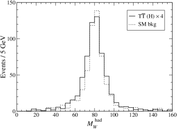
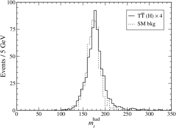
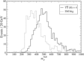
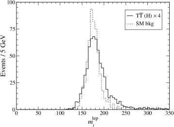
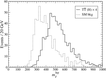
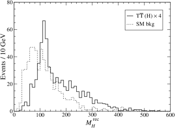
Figure 9: Analysis II ($5b$, $6b$ final states): Reconstructed masses of the hadronic $W$, the hadronic and leptonic top and heavy quarks and the Higgs boson, for the background and the sum of $T\bar{T}$ Higgs signals.

In these final states the SM background is already very small, and performing kinematical cuts on reconstructed Higgs and heavy quark masses or light jet multiplicity can easily reduce the signal significance. Therefore, for this analysis we include these variables in the likelihood functions, and only perform loose cuts on the signal likelihood. The variables used are $m_{T}^{\mathrm{had}}$, $m_{T}^{\mathrm{lep}}$, $M_{H}^{\mathrm{rec}}$, $m_{bb}^{(1)}$, $H_{T}$, $p_{t}^{b,\mathrm{max}}$, $p_{t}^{b,\mathrm{max2}}$, and $p_{t}^{j,\mathrm{max2}}$, defined in the previous subsection, the jet multiplicity and the the charged lepton transverse momentum $p_{t}^{\mathrm{lep}}$. We only use two classes, for the $T\bar{T}\,(HH)$ signal and the background, and the same distributions are used for final states with 5 and 6 $b$ quarks. The normalised variables are presented in Fig. 10 except $H_{T}$ and $p_{t}^{b,\mathrm{max}}$ which are very similar to the plots in Fig. 7 and the jet multiplicity, shown in Fig. 5. The log-likelihood function is also presented in Fig. 10. We point out that the signal likelihood for the $T\bar{T}\,(WH)$ and $T\bar{T}\,(ZH)$ processes is very high even without using a separate class for them.

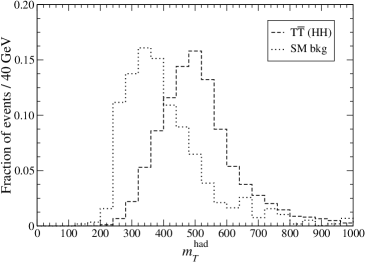
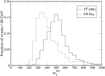
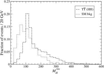
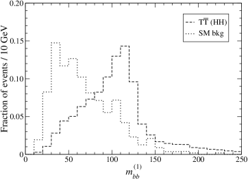
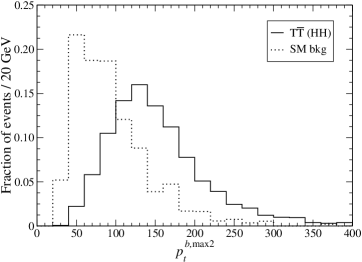
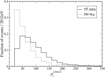
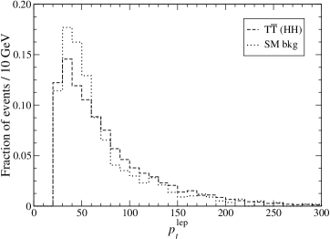
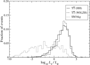
Figure 10: Analysis II ($5b$, $6b$ final states): Normalised variables $m_{T}^{\mathrm{had}}$, $m_{T}^{\mathrm{lep}}$, $M_{H}^{\mathrm{rec}}$, $m_{bb}^{(1)}$, $p_{t}^{b,\mathrm{max2}}$, $p_{t}^{j,\mathrm{max2}}$ and $p_{t}^{\mathrm{lep}}$, used in the likelihood analysis. Log-likelihood function.

We suppress the background by requiring

$$\log_{10}L_{S}/L_{B}\geq 2.6 (5b)\,,$$

$$\log_{10}L_{S}/L_{B}\geq 0 (6b)\,.$$ (18)

The number of events after these cuts are collected in Table 7. For 30 fb^-1 of luminosity, the statistical significance of the Higgs signal is $\mathcal{S}_{20}=6.02\sigma$, $\mathcal{S}_{20}=5.63\sigma$ for $5b$ and $6b$ final states, respectively. We observe that the $t\bar{t}b\bar{b}$ background acquires increasing relevance in these final states with five and six $b$-tagged jets. In order to have a good estimate of the effect of higher order processes $t\bar{t}b\bar{b}j$, $t\bar{t}b\bar{b}jj$, etc. we have included a factor $k=2.05$ into its tree-level cross section, as explained in section 3. However, the kinematics of the higher order processes might be important and a detailed simulation (when a Monte Carlo generator including a matching prescription for these processes is available) is needed to confirm these results. Besides, we have explicitly checked that the $t\bar{t}b\bar{b}b\bar{b}$ background, not included in our simulations, is negligibly small.

	$N_{\text{cut}}^{(5)}$	$N_{\text{cut}}^{(6)}$			$N_{\text{cut}}^{(5)}$	$N_{\text{cut}}^{(6)}$
$T\bar{T}\,(WH)$	13.3	2.0		$t\bar{t}b\bar{b}$	8	7
$T\bar{T}\,(HH)$	23.4	17.6		$t\bar{t}c\bar{c}$	0	0
$T\bar{T}\,(ZH)$	8.1	4.6		$t\bar{t}b\bar{b}$ EW	1.4	0.3
$T\bar{T}\,(WZ)$	1.6	0.4		$t\bar{t}b\bar{b}$ EW ($T$)	0.9	0.5
$T\bar{T}\,(WZ)$ ($H\!\!\!\!\!\!\!\not\,\,\,\,\,$)	3.5	0.7		$t\bar{t}c\bar{c}$ EW	0.0	0.0
$T\bar{T}\,(ZZ)$	0.6	0.2		$t\bar{t}c\bar{c}$ EW ($T$)	0.0	0.0
$T\bar{T}\,(ZZ)$ ($H\!\!\!\!\!\!\!\not\,\,\,\,\,$)	1.2	0.6		$Wjjjjjj$	0	0
$T\bar{T}b\bar{b}$	0.1	0.0		$Wb\bar{b}jjjj$	2	1
$T\bar{T}b\bar{b}$ ($H\!\!\!\!\!\!\!\not\,\,\,\,\,$)	0.1	0.0		$Wc\bar{c}jjjj$	0	0
$t\bar{t}H$ ($T$)	1.4	0.3		$Wb\bar{b}b\bar{b}$	0	0
$t\bar{t}$	0	0		$Zjjjjjj$	0	0
$t\bar{t}j$	2	1		$Zb\bar{b}jjjj$	0	0
$t\bar{t}2j$	0	0		$Zc\bar{c}jjjj$	0	0
$t\bar{t}3j$	0	0
$t\bar{t}4j$	1	0
$t\bar{t}5j$	7	1

Table 7: Analysis II ($5b$, $6b$ final states): Number of events (for 30 fb^-1) after the selection cuts in Eqs. (18)

4.2.3 Summary

For a luminosity of 30 fb^-1, the statistical significances of the three channels (including a 20% background systematic uncertainty) are

$$4b: \quad S_{20}=6.43\sigma\,,$$

$$5b: \quad S_{20}=6.02\sigma\,,$$

$$6b: \quad S_{20}=5.63\sigma\,.$$ (19)

When the three channels are combined, a statistical significance of $10.45\sigma$ is obtained for the $T\bar{T}$ Higgs signals. This is a factor of 25 better than for $t\bar{t}H$ production, and offers a good opportunity to quickly discover the Higgs boson in final states containing a charged lepton and four or more $b$ quarks. Rescaling the expected signal and background rates (and using Poisson statistics) it is found that a $5\sigma$ discovery could be achieved approximately for 8 fb^-1. This represents a reduction in luminosity by more than one order of magnitude with respect to $t\bar{t}H$ production in all $t\bar{t}$ decay channels, and might be improved with less restrictive selection cuts. This high sensitivity is due not only to the large $T\bar{T}$ cross section, but also to the distinctive features of this signal, characterised by large transverse momenta, high $b$ jet multiplicity and reconstructed invariant masses peaking at $m_{T}$. At any rate, a likelihood analysis must be employed to benefit from the distinctive kinematics and separate these signals from the $t\bar{t}nj$ background, which also involves large transverse momenta for higher values of $n$.

We finally comment on the experimental observation of the Higgs boson from $T\bar{T}$ decays. Although the reconstruction of the final state does not explicitly make use of the new quark mass, the distributions used in the probabilistic analysis do. Since the mass of an eventual heavy quark $T$ is unknown, two alternatives are possible for the experimental search: (i) generate sets of distributions and build likelihood functions for different values of $m_{T}$ and compare them with real data; (ii) set generic kinematical cuts and look for peaks in the invariant mass distributions. The second approach gives sensitivities similar or worse than the ones obtained in this section, and the analysis has been omitted for brevity. For illustration, in the next section we will show how the new quark can be discovered with the observation of peaks in the $m_{T}^{\mathrm{had}}$, $m_{T}^{\mathrm{lep}}$ distributions.

5 Heavy quark discovery

Discovering the Higgs boson from $T\bar{T}$ decays implies the discovery of the new quark. However, as emphasised in the paragraph before Eq. (16), the significances for the Higgs and $T$ quark discoveries are different, due to the different classification of signals and backgrounds. Using the data in Tables 6, 7 and taking $t\bar{t}H$ as part of the background, the significances for $T$ discovery with 30 fb^-1 are

$$4b: \quad S_{20}=6.93\sigma\,,$$

$$5b: \quad S_{20}=7.09\sigma\,,$$

$$6b: \quad S_{20}=6.28\sigma\,,$$ (20)

with a combined significance $S_{20}=11.74\sigma$. $5\sigma$ evidence of the new quark (always assuming $m_{T}=500$ GeV) could be achieved for 7 fb^-1.

It is also interesting to discover the new quark by observing peaks in the $m_{T}^{\mathrm{had}}$, $m_{T}^{\mathrm{lep}}$ distributions. Quantifying the confidence level of such peaks, so as to claim discovery, requires an appropriate background normalisation. The procedure used here follows and extends the one proposed in Ref. [47] for detecting anomalous couplings. Performing a $\chi^{2}$ fit to the binned data, a background rescaling factor $\kappa$ can be obtained by minimising the quantity

$$\chi^{2}=\sum_{i}\frac{(N_{i}-\kappa B_{i})^{2}}{\kappa B_{i}}\,,$$ (21)

where $i$ sums over the bins, $N_{i}$ are the numbers of events observed and $B_{i}$ the expected background. The minimum is found for

$$\kappa^{2}=\frac{1}{B}\sum_{i}\frac{N_{i}^{2}}{B_{i}}\,,$$ (22)

where $B=\sum_{i}B_{i}$ is the total expected background. Since in a real experiment the number of events observed will include not only the background but also a part from the signal itself, in most cases $\kappa>1$ will be found. The uncertainty in this normalisation factor is given by

$$\delta\kappa^{2}=\left[\frac{3\kappa^{4}}{B}+\frac{1}{B^{2}}\sum_{i}\frac{N_{i}^{4}}{B_{i}^{3}}\right]^{1/2}\,.$$ (23)

For a single bin we have $\kappa=N/B$, $\delta\kappa/\kappa=1/\sqrt{B}$, as expected. The statistical significance of the signal at the peak is

$$\mathcal{S}_{\kappa}\equiv S^{\prime}/\sqrt{\kappa B+(\delta\kappa B)^{2}}\,,$$ (24)

where $S^{\prime}<S$ is the excess of events over the rescaled background. The second term in the square root is a background normalisation systematic error, arising from the uncertainty in the determination of $\kappa$. For a sufficiently large number of events, $\delta\kappa\sim\kappa/\sqrt{B}$ is smaller than the assumed 20% systematic error in the total cross section. On the other hand, this approach has the drawback that the significance is determined by $S^{\prime}$, which may be significantly smaller than $S$ if off-peak signal contributions (combinatorial background) are large, and the “effective” statistical error in the background is $\sqrt{\kappa B}$. Besides, this background rescaling assumes that the main sources of systematic error (e.g. $b$ and light jet tagging efficiencies, jet energy resolution, etc.) do not significantly affect the shape of the relevant distribution in which the peak is observed.

The probabilistic analysis in section 4.2 is not the best suited for detecting the peaks in the $m_{T}^{\mathrm{had}}$, $m_{T}^{\mathrm{lep}}$ distributions. Even not including these variables in the likelihood functions, requiring a high signal likelihood biases the background, concentrating the distributions of $m_{T}^{\mathrm{had}}$ and $m_{T}^{\mathrm{lep}}$ around $m_{T}=500$ GeV. This is not completely unexpected, since the signal distributions of the total transverse energy, missing momentum, etc. have been obtained assuming $m_{T}=500$ GeV. Therefore, instead of a likelihood analysis we perform one based on simple kinematical cuts. We restrict ourselves to final states with 4 $b$-tagged jets (in the $5b$ and $6b$ channels the background rescaling has a larger uncertainty due to the smaller statistics). We require

$$H_{T} \geq 1000~{}\text{GeV}\,,$$

$$p_{t}^{b,\mathrm{max}} \geq 100~{}\text{GeV}\,,$$

$$\mathcal{N}_{\text{jet}} \leq 7$$ (25)

to reduce the background. The reconstructed mass distributions obtained are presented in Fig. 11. The SM background is normalised with cross section measurements in the regions $160~{}\text{GeV}\leq m_{T}^{\mathrm{had}},m_{T}^{\mathrm{lep}}\leq 360$ GeV, $680~{}\text{GeV}\leq m_{T}^{\mathrm{had}},m_{T}^{\mathrm{lep}}\leq 840$ GeV, obtaining similar rescaling factors in both distributions, $\kappa=1.139\pm 0.051$ and $\kappa=1.141\pm 0.050$ respectively. Within the mass windows

$$360~{}\text{GeV}\leq m_{T}^{\mathrm{had}},m_{T}^{\mathrm{lep}}\leq 640~{}\text{GeV}$$ (26)

the significance of the signal (over the rescaled background) is $\mathcal{S}_{\kappa}=4.27\sigma$. (The total number of events after the cuts in Eqs. (25) and the events in the peak regions can be read in Table 8.) In this example we find a smaller sensitivity with this method than with the probabilistic analysis used in section 4.2, which was $\mathcal{S}_{20}=6.93\sigma$. Nevertheless, it has the aesthetical advantage of being able to observe the peaks corresponding to the new quark with unbiased background.

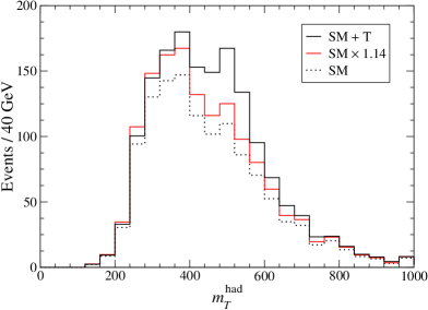
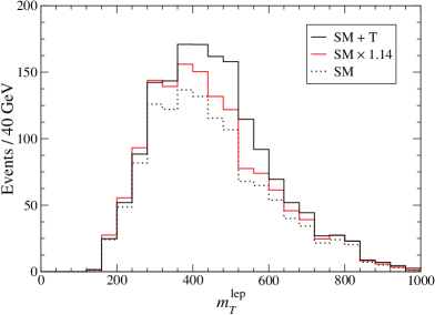
Figure 11: Reconstructed heavy quark masses after the kinematical cuts in Eqs. (25). The dotted lines represent the SM background, and the red lines the same but rescaled by factor $\kappa\simeq 1.14$. The continuous lines correspond to the background plus all heavy quark signals.

	$N_{\text{cut}}$	$N_{\text{peak}}$			$N_{\text{cut}}$	$N_{\text{peak}}$
$T\bar{T}\,(WH)$	193.9	137.6		$t\bar{t}b\bar{b}$	223	104
$T\bar{T}\,(HH)$	80.0	43.0		$t\bar{t}c\bar{c}$	43	20
$T\bar{T}\,(ZH)$	48.7	27.2		$t\bar{t}b\bar{b}EW$	17.5	7.8
$T\bar{T}\,(WZ)$	23.7	15.5		$t\bar{t}c\bar{c}EW$	1.3	1.0
$T\bar{T}\,(ZZ)$	4.5	2.2		$Wjjjjjj$	4	1
$T\bar{T}b\bar{b}$	1.2	0.6		$Wb\bar{b}jjjj$	33	11
$t\bar{t}H$	26.2	10.0		$Wc\bar{c}jjjj$	6	1
$t\bar{t}$	36	15		$Wb\bar{b}b\bar{b}$	1	1
$t\bar{t}j$	75	33		$Zjjjjjj$	0	0
$t\bar{t}2j$	178	61		$Zb\bar{b}jjjj$	7	4
$t\bar{t}3j$	243	105		$Zc\bar{c}jjjj$	0	0
$t\bar{t}4j$	222	100
$t\bar{t}5j$	135	58

Table 8: Number of events with 4 $b$ tags (for 30 fb^-1) after the selection cuts in Eqs. (25) ($N_{\text{cut}}$) and also within the mass windows in Eq. (26) ($N_{\text{peak}}$).

6 Other results

We conclude this analysis examining the dependence of our results on some of our assumptions. We can estimate how our results change if: (i) we use MRST structure functions [48]; (ii) we include the charged lepton identification efficiency; (iii) we select $b$ tagging efficiencies of 50% or 70%; (iv) a systematic uncertainty of 30% is assumed in the background. In the first case we compute the significances rescaling the numbers of events in Tables 4–7 by factors reflecting the change in the cross sections. In the second case we naively use an average charged lepton identification efficiency of 90%. For the third, we provide crude estimates based on rescaling by the nominal $b$ tagging efficiencies and rejection factors. The resulting significances for the Higgs signals are collected in Table 9. For the $T$ discovery in the $4b$, $5b$ and $6b$ channels they are slightly larger, as shown in the previous section.

	$t\bar{t}H$	$T\bar{T}(H,4b)$	$T\bar{T}(H,5b)$	$T\bar{T}(H,6b)$
Standard	0.39	6.43	6.02	5.63
MRST	0.38	7.30	6.73	6.45
$\ell$ eff. 90%	0.38	6.24	5.86	5.41
$b$ eff. 50%	0.68	6.28	5.41	4.80
$b$ eff. 70%	0.12	1.74	1.70	1.81
sys 30%	0.31	5.08	4.72	4.78

Table 9: Estimates of the Higgs signal significances under different assumptions, explained in the text.

The results are rather stable except for a 70% $b$ tagging efficiency, where backgrounds grow due to the larger mistagging rate. For a slightly different Higgs mass the results are stable too, as long as the decay $H\to b\bar{b}$ dominates, and an additional (small) dependence on $M_{H}$ is through the branching ratios for $T$ decays, plotted in Fig. 2. For larger $T$ masses the signal is suppressed (and for lighter $T$ enhanced) as a consequence of the variation in the $T\bar{T}$ cross section, plotted in Fig. 1. For instance, for a heavy quark mass $m_{T}=600$ GeV the cross section is 776 fb, almost three times smaller than for $m_{T}=500$ GeV. On the other hand, the SM background decreases for larger transverse momenta, but the latter effect does not make up for the reduction in the $T\bar{T}$ cross section.

7 Summary

Heavy singlet decays were recognised early as an important source of Higgs bosons [14], with a branching ratio close to 25% for $M_{H}\ll m_{T}$. In this work we have addressed their experimental observation at LHC, assuming a Higgs mass of 115 GeV and the possible existence of a 500 GeV heavy quark $T$. We have performed a detailed signal and background study, with matrix-element-based generators for the hard processes, subsequent parton showering and hadronisation by PYTHIA and a fast simulation of the ATLAS detector. As a by-product, new leading-order event generators for $t\bar{t}b\bar{b}$, $t\bar{t}c\bar{c}$, $t\bar{t}H$, $Wb\bar{b}b\bar{b}$ and other processes have been developed. These generators include top quark, $W$ and Higgs boson decays and take finite width and spin effects into account. Their output provides the colour information necessary for hadronisation.

In our analysis we have first reevaluated the discovery potential of $t\bar{t}H$ production, with $H\to b\bar{b}$ and semileptonic decay of the $t\bar{t}$ pair, in the SM. Our result, $0.4\sigma$ significance for 30 fb^-1 in low luminosity running, is similar to the most recent one by CMS, although the details of the analysis (full simulation for the CMS analysis, with inclusion of a $K$ factor for $t\bar{t}H$) differ. Both results are substantially more pessimistic than earlier ones [5, 7, 8], because in previous studies only the lowest orders of the leading $t\bar{t}nj$ background were taken into account, and systematic uncertainties in the background normalisation were not considered. The $b$ tagging performance has a large impact on the final result, especially regarding the dominant $t\bar{t}nj$ background. We have used the efficiencies implemented in ATLFASTB for the low luminosity run: 60% $b$ tagging rate and nominal rejection factors of $6.7$ for charm and $93$ for light jets (with $p_{t}$-dependent corrections). If the latter are better than expected, the observability of $t\bar{t}H$ production will improve. In this respect, full simulations of matrix-element-generated signals and backgrounds would be welcome, but it is not likely that results will attain observability of $t\bar{t}H$. Results also depend to some extent on the ability to reconstruct invariant masses. With a full simulation the mass reconstruction may be degraded, although studies performed for top pair production have shown good agreement between fast and full simulations, not only for reconstructed masses but also for angular distributions [42]. On the other hand, it must be pointed out that our results are conservative in the sense that higher multiplicity backgrounds $t\bar{t}nj$ are included but not higher multiplicity signal processes $t\bar{t}Hnj$. The latter might improve the observability by a factor of two.

New Higgs signals from $T\bar{T}$ decays, $T\bar{T}\to W^{+}b\,H\bar{t}/Ht\,W^{-}\bar{b}$, $T\bar{T}\to Ht\,H\bar{t}$ and $T\bar{T}\to Zt\,H\bar{t}/Ht\,Z\bar{t}$, have been then examined. We have demonstrated that, in a standard search for $t\bar{t}H$ production, a possible contribution of these processes can easily be overlooked, and do not much improve the Higgs observability. We have presented a novel reconstruction technique specific to the search for the leading signals $T\bar{T}\to W^{+}b\,H\bar{t}/Ht\,W^{-}\bar{b}\to W^{+}bW^{-}\bar{b}H$, $T\bar{T}\to Ht\,H\bar{t}\to W^{+}bW^{-}\bar{b}HH$, which does not require knowledge of the heavy quark mass. Despite their different kinematics and large transverse momenta, these signals are not easy to isolate from the $t\bar{t}nj$ background, which is large and also involves larger transverse momenta for increasing values of $n$. Using a likelihood analysis, these processes are cleanly separated from the SM background, giving a high statistical significance for the Higgs, $10.4\sigma$ for 30 fb^-1 including a 20% systematic uncertainty in the background normalisation. In the case that a 500 GeV $T$ quark exists, 8 fb^-1 of luminosity could suffice to discover the Higgs boson. This striking signal is due to the large $T\bar{T}$ production cross section (2.14 pb for $m_{T}=500$ GeV), the large branching ratio for final states with Higgs bosons, $\text{Br}(T\bar{T}\to H+X)=0.55$, and the distinctive features of these processes: in addition to larger transverse momenta, a high $b$ jet multiplicity in the final state and reconstructed invariant masses peaking at $m_{T}$.

Finally, we have addressed the observability of the new quark, which is not equivalent to the discovery of the Higgs boson because the classification of processes as signals and background differs. We have shown that a significance of $11.7\sigma$ is reached for 30 fb^-1, similar to the one in the $T\bar{T}\to W^{+}bW^{-}\bar{b}$ channel (a detailed comparison between both channels is difficult because of the different assumptions made in the two studies). We have also used a standard analysis in order to show that the peaks in the invariant mass distributions of the heavy quarks would be easy to observe, even considering the uncertainties in the background normalisation. For higher $T$ masses, $T\bar{T}\to W^{+}bW^{-}\bar{b}$ is the leading discovery channel, due to three facts: (i) the branching ratio for $\ell\nu bbbbjj$ final states decreases slightly with $m_{T}$; (ii) for heavier $T$, the charged lepton from the semileptonic decay $T\to W^{+}b\to\ell^{+}\nu b$ (or the charge conjugate) generically has a very large transverse momentum which can be exploited to reduce backgrounds very efficiently [46]; (iii) larger $T$ masses can only be explored in a high luminosity LHC run, where $b$ tagging performance is degraded and multi-jet backgrounds to the $T\bar{T}(WH,HH,ZH)$ signals are larger.

Acknowledgements

I thank F. del Aguila and R. Pittau for useful discussions and for reading the manuscript, and the referee for many useful suggestions. This work has been supported by a MEC Ramon y Cajal contract and project FPA 2003-09298-C02-01, and by Junta de Andalucía projects FQM 101 and FQM 437.

Appendix A Probabilistic analysis

In the probabilistic analysis we build likelihood functions which use information from several kinematical variables to discriminate between event classes, namely the signal (one or more) and the background. For a given kinematical variable $x$, e.g. a transverse momentum, different event classes $j=1,\dots,m$ have different kinematical distributions $f^{j}(x)$, which we normalise to unity. We define the “probability” function

$$p_{j}(x)=\frac{f_{j}(x)}{\sum_{k}f_{k}(x)}\,.$$ (27)

If the distributions $f^{j}$ are normalised to their total cross section, the function $p^{j}(x)$ represents the probability that the event corresponds to the class $j$, and when normalised to unity $p^{j}$ it is the relative probability (up to total cross section factors). For a set of kinematical variables $x_{i}$, $i=1,\dots,n$, the likelihoods $L_{j}$ are then defined as the product of the probabilities for each variable $x_{i}$,

$$L_{j}(x_{1},\dots,x_{n})=\prod_{i=1}^{n}p_{j}^{i}(x_{i})\quad j=1,\dots,m\,.$$ (28)

Selection cuts may be applied on likelihood ratios $L_{S_{i}}/L_{B}$, for $S_{i}$ and $B$ the signal and background classes, respectively, in order to enhance the signal(s). Alternatively, instead of working directly with these ratios it is often more practical to consider the logarithm of these quantities, $\log_{10}L_{S_{i}}/L_{B}$.

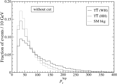
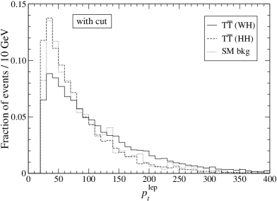
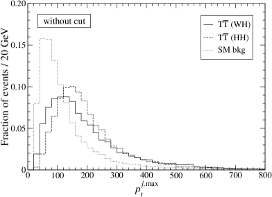
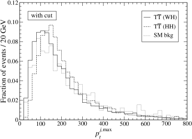
Figure 12: Normalised variables $p_{t}^{\mathrm{lep}}$, $p_{t}^{j,\mathrm{max}}$ for the analysis II ($4b$ final states), without cuts and after requiring $\log_{10}L_{S}/L_{B}\geq 2$, with $L_{S}$, $L_{B}$ involving the rest of variables.

We emphasise that performing a probabilistic analysis of this type is not as straightforward as one might think. Naively, one would take all the relevant variables which exhibit different distributions for signal and background and build with them likelihood functions. But this is not optimal and, perhaps surprisingly, some variables which one might consider as relevant actually reduce the discriminating power of the likelihood functions. This can be understood as a result of the fact that some variables are correlated, and selecting values of one of them modifies the distribution of the others. Let us take as example the transverse momentum distributions of the charged lepton ($p_{t}^{\mathrm{lep}}$) and the light jet with maximum $p_{t}$ ($p_{t}^{j,\mathrm{max}}$) for the analysis II in $4b$ final states. These variables have not been included in the probabilistic analysis in this case. Their normalised distributions before any cut are presented in Fig. 12 (left), and after requiring $\log_{10}L_{S}/L_{B}>2$ (but without them on the likelihood functions) on the right. From their distributions in the left column we observe that their inclusion in the likelihood functions would favour larger transverse momenta, since the background distributions are peaked at lower $p_{t}$. But observing the right column we realise that this would actually disfavour the signal over the background (for example, the tail in the $p_{t}^{j,\mathrm{max}}$ distribution after the likelihood cut is larger for the background than for the two signals, and in the $p_{t}^{\mathrm{lep}}$ distribution larger for the background than for $T\bar{T}\,(HH)$). These examples make apparent that optimising the analysis requires educated guessing and trial and error to find (or get close to) the best set of variables.

References

- [1] P. W. Higgs, Broken Symmetries And The Masses Of Gauge Bosons, Phys. Rev. Lett. 13 (1964) 508; Spontaneous Symmetry Breakdown Without Massless Bosons, Phys. Rev. 145 (1966) 1156.
- [2] R. Barate et al. [LEP Working Group for Higgs boson searches], Search for the standard model Higgs boson at LEP, Phys. Lett. B 565 (2003) 61 [hep-ex/0306033].
-
[3]
LEP Electroweak Working group,
A combination of preliminary electroweak measurements and constraints on
the standard model,
hep-ex/0511027;
see also
http://lepewwg.web.cern.ch/LEPEWWG - [4] N. Cabibbo, L. Maiani, G. Parisi and R. Petronzio, Bounds On The Fermions And Higgs Boson Masses In Grand Unified Theories, Nucl. Phys. B 158 (1979) 295.
- [5] ATLAS collaboration, ATLAS detector and physics performance technical design report, CERN-LHCC-99-15.
- [6] CMS collaboration, CMS Physics technical design report volume II: Physics Performance, CERN-LHCC-2006-021.
- [7] J. Cammin and M. Schumacher, The ATLAS discovery potential for the channel , , ATLAS note ATL-PHYS-2003-024.
- [8] B. King, S. Maxfield and J. Vossebeld, Search for a light Standard Model Higgs in the channels , ATLAS note ATL-PHYS-2004-031.
- [9] S. Cucciarelli et al., em Search for in association with a pair at CMS, CMS note 2006/119
- [10] S. Asai et al., Prospects for the search for a standard model Higgs boson in ATLAS using vector boson fusion, Eur. Phys. J. C 32S2 (2004) 19 [hep-ph/0402254].
- [11] K. Jakobs and T. Trefzger, SM Higgs Searches for with a Mass between GeV at LHC, ATLAS note ATL-PHYS-2000-015.
- [12] B. Mohn and B. Stugu, Corrections to the discovery potential for finding the Standard Model Higgs in the four lepton final state, ATLAS note ATL-PHYS-2004-014.
- [13] C. R. Chen, K. Tobe and C. P. Yuan, Higgs boson production and decay in little Higgs models with T-parity, hep-ph/0602211.
- [14] F. del Aguila, G. L. Kane and M. Quiros, A Possible Method To Produce And Detect Higgs Bosons At Hadron Colliders, Phys. Rev. Lett. 63 (1989) 942; F. del Aguila, L. Ametller, G. L. Kane and J. Vidal, Vector Like Fermion And Standard Higgs Production At Hadron Colliders, Nucl. Phys. B 334 (1990) 1.
- [15] N. Arkani-Hamed, A. G. Cohen and H. Georgi, Electroweak symmetry breaking from dimensional deconstruction, Phys. Lett. B 513 (2001) 232 [hep-ph/0105239]; N. Arkani-Hamed, A. G. Cohen, E. Katz and A. E. Nelson, The littlest Higgs, JHEP 0207 (2002) 034 [hep-ph/0206021].
- [16] E. A. Mirabelli and M. Schmaltz, Yukawa hierarchies from split fermions in extra dimensions, Phys. Rev. D 61 (2000) 113011 [hep-ph/9912265]; S. Chang, J. Hisano, H. Nakano, N. Okada and M. Yamaguchi, Bulk standard model in the Randall-Sundrum background, Phys. Rev. D 62 (2000) 084025 [hep-ph/9912498]; F. del Aguila and J. Santiago, Universality limits on bulk fermions, Phys. Lett. B 493 (2000) 175 [hep-ph/0008143].
- [17] P. H. Frampton, P. Q. Hung and M. Sher, Quarks and leptons beyond the third generation, Phys. Rept. 330 (2000) 263 [hep-ph/9903387].
- [18] J. A. Aguilar-Saavedra, Pair production of heavy singlets at LHC, Phys. Lett. B 625 (2005) 234 [Erratum-ibid. B 633 (2006) 792] [hep-ph/0506187].
- [19] R. Mehdiyev, S. Sultansoy, G. Unel and M. Yilmaz, Search for E6 isosinglet quarks in ATLAS, hep-ex/0603005.
- [20] E. Arik, M. Arik, S. A. Cetin, T. Conka, A. Mailov and S. Sultansoy, With four standard families, the LHC could discover the Higgs boson with a few fb-1, Eur. Phys. J. C 26 (2002) 9 [hep-ph/0109037].
- [21] F. del Aguila and M. J. Bowick, The Possibility Of New Fermions With Mass, Nucl. Phys. B 224 (1983) 107.
- [22] P. Langacker and D. London, Mixing Between Ordinary And Exotic Fermions, Phys. Rev. D 38 (1988) 886.
- [23] V. D. Barger, M. S. Berger and R. J. N. Phillips, Quark singlets: Implications and constraints, Phys. Rev. D 52 (1995) 1663 [hep-ph/9503204].
- [24] J. A. Aguilar-Saavedra, Effects of mixing with quark singlets, Phys. Rev. D 67 (2003) 035003 [Erratum-ibid. D 69 (2004) 099901] [hep-ph/0210112].
-
[25]
CDF Collaboration,
Search for heavy Top in Lepton Plus Jets events,
CDF note 8003; see also
http://www-cdf.fnal.gov/physics/new/top/2005/ljets/tprime/gen6/public.html - [26] W. M. Yao et al. [Particle Data Group], Review of particle physics, J. Phys. G 33 (2006) 1.
- [27] F. del Aguila, J. A. Aguilar-Saavedra and R. Miquel, Constraints on top couplings in models with exotic quarks, Phys. Rev. Lett. 82 (1999) 1628 [hep-ph/9808400].
- [28] G. Azuelos et al., Exploring little Higgs models with ATLAS at the LHC, Eur. Phys. J. C 39S2 (2005) 13 [hep-ph/0402037].
- [29] T. Sjostrand, S. Mrenna and P. Skands, PYTHIA 6.4 physics and manual, JHEP 0605 (2006) 026 [hep-ph/0603175].
- [30] M. L. Mangano, M. Moretti, F. Piccinini, R. Pittau and A. D. Polosa, ALPGEN, a generator for hard multiparton processes in hadronic collisions, JHEP 0307 (2003) 001 [hep-ph/0206293]; See also http://mlm.home.cern.ch/m/mlm/www/alpgen/
- [31] M. L. Mangano, talk at Lund University, http://cern.ch/ mlm/talks/lund-alpgen.pdf
- [32] S. Jadach, Z. Was, R. Decker and J. H. Kuhn, The decay library TAUOLA: Version 2.4, Comput. Phys. Commun. 76 (1993) 361.
- [33] E. Barberio, B. van Eijk and Z. Was, Photos: A Universal Monte Carlo For QED Radiative Corrections In Decays, Comput. Phys. Commun. 66 (1991) 115.
- [34] E. Richter-Was, D. Froidevaux and L. Poggioli, ATLFAST 2.0 a fast simulation package for ATLAS, ATLAS note ATL-PHYS-98-131.
- [35] E. Murayama, I. Watanabe and K. Hagiwara, HELAS: HELicity Amplitude Subroutines for Feynman Diagram Evaluations, KEK report 91-11, January 1992.
- [36] T. Stelzer and W. F. Long, Automatic generation of tree level helicity amplitudes, Comput. Phys. Commun. 81 (1994) 357 [hep-ph/9401258].
- [37] B. P. Kersevan and E. Richter-Was, The Monte Carlo event generator AcerMC version 2.0 with interfaces to PYTHIA 6.2 and HERWIG 6.5, hep-ph/0405247.
- [38] G. P. Lepage, Vegas: An Adaptive Multidimensional Integration Program, Report CLNS-80/447.
- [39] H. L. Lai et al. [CTEQ Collaboration], Global QCD analysis of parton structure of the nucleon: CTEQ5 parton distributions, Eur. Phys. J. C 12 (2000) 375 [hep-ph/9903282].
- [40] R. Barate et al. [ALEPH Collaboration], Studies of quantum chromodynamics with the ALEPH detector, Phys. Rept. 294 (1998) 1.
- [41] A. I. Etienvre, J. P. Meyer and J. Schwindling, Top quark mass measurement in the lepton plus jet channel using full simulation, ATLAS note ATL-PHYS-INT-2005-002.
- [42] F. Hubaut, E. Monnier, P. Pralavorio, B. Resende and C. Zhu, Comparison between full and fast simulations in top physics, ATLAS note ATL-PHYS-PUB-2006-017.
- [43] For a recent comparison see F. Hubaut, E. Monnier, P. Pralavorio, B. Resende and C. Zhu, Polarization studies in semileptonic events with ATLAS full simulation, ATLAS note ATL-PHYS-PUB-2006-022.
- [44] CMS collaboration, CMS Physics technical design report volume I: Detector Performance and Software, CERN-LHCC-2006-001.
- [45] T. Schörner-Sadenius and S. Tapprogge, ATLAS Trigger Menus for the LHC Start-up Phase, ATLAS note ATL-DAQ-2003-004.
- [46] J. A. Aguilar-Saavedra, New signals in pair production of heavy singlets at LHC, hep-ph/0603199.
- [47] U. Baur and E. L. Berger, Probing The Weak Boson Sector In Z Gamma Production At Hadron Colliders, Phys. Rev. D 47 (1993) 4889.
- [48] A. D. Martin, R. G. Roberts, W. J. Stirling and R. S. Thorne, Physical gluons and high- jets, Phys. Lett. B 604 (2004) 61 [hep-ph/0410230].