New signals in pair production of heavy $Q=2/3$ singlets at LHC

Abstract:

New quark singlets $T$ can be produced in pairs at LHC through standard QCD interactions, with a large cross section for masses of several hundreds of GeV. Their charged current decays $T\bar{T}\to W^{+}b\,W^{-}\bar{b}$, with semileptonic decay of the $W$ pair, give a final state $\ell\nu bbjj$, as in top pair production. The mixed decay modes $T\bar{T}\to W^{+}b\,H\bar{t},Ht\,W^{-}\bar{b}\to W^{+}bW^{-}\bar{b}H$, $T\bar{T}\to W^{+}b\,Z\bar{t},Zt\,W^{-}\bar{b}\to W^{+}bW^{-}\bar{b}Z$, with $H,Z\to jj$, yield two more jets, $\ell\nu bbjjjj$, or the same state in the latter case for $Z\to\nu\bar{\nu}$. We extend previous work examining in detail the extra $H$ and $Z$ contributions and stressing one of the salient features of the $T\bar{T}\to W^{+}b\,W^{-}\bar{b}$ signal: the presence of a very energetic charged lepton. We finally compare with the discovery potential in $\ell\nu bbbbjj$ final states, with four $b$ tags.

1 Introduction

Fermion singlets under $\mathrm{SU}(2)_{L}$ are not present in the minimal Standard Model (SM); however, their existence is experimentally allowed, provided their mixing with the standard fermions is of order $O(0.1)$ or smaller. By far, the best known example in which singlet fermions are postulated is the seesaw mechanism, where neutrino singlets are introduced to explain the smallness of neutrino masses. Quark singlets appear in some SM extensions like those with extra dimensions [1], in grand unified theories [2, 3] and Little Higgs models [4]. In analogy with the neutrino case, the existence of one $Q=2/3$ singlet $T$ (or more) could provide a clue to understand the largeness of the top mass [5, 6].

The possible existence of a $Q=2/3$ singlet $T$ with a mass of several hundreds of GeV would have very interesting phenomenological consequences. Its mixing with the top and up or charm quarks would generate flavour-changing neutral couplings at the tree level, large enough to be detectable at the Large Hadron Collider (LHC) [7, 8]. In low energy processes, its contribution could lead to significant departures from SM predictions for several observables, like rare kaon decays, $D^{0}-\bar{D}^{0}$ mixing and CP asymmetries in $B$ oscillations [8, 9, 10, 11], compatible with present experimental measurements. But the most interesting “indirect effect” of a quark singlet is Higgs boson discovery [12, 13]: in the presence of a heavy singlet, the luminosity required for Higgs discovery at LHC is dramatically reduced. For instance, for $m_{T}=500$ GeV, the luminosity needed for discovery of a 115 GeV Higgs is only 6 fb^-1 [14], ten times smaller than within the minimal SM.

Besides their indirect effects, $Q=2/3$ singlets can be directly observed at LHC. They can be produced in pairs by QCD interactions [3, 13], or in association with a light jet, through its mixing with the bottom quark $V_{Tb}$ [15, 16]. Both processes have their own advantages and weaknesses. Pair production has a model-independent cross section determined by QCD interactions, which however decreases quickly with $m_{T}$, due to phase space suppression. Single $T$ production cross section decreases more slowly with the heavy quark mass, but on the other hand it is proportional to $|V_{Tb}|^{2}$, and gets suppressed for small mixings. Branching ratios for $T\bar{T}$ final states involve two heavy quark decays and are thus smaller than for $Tj$ production. But they also have more fermions in the final state, and then their backgrounds are less important. A heavy quark $T$ can decay via charged currents $T\to W^{+}b$, neutral currents $T\to Zt$ and, if the Higgs boson is light enough, $T\to Ht$ as well. The decay widths are approximately $\mathrm{Br}(T\to W^{+}b)=0.5$, $\mathrm{Br}(T\to Zt)=0.25$, $\mathrm{Br}(T\to Ht)=0.25$ (these figures are exact for $m_{T}\gg M_{W},M_{Z},M_{H}$). We neglect decays to first and second generation quarks, involving mixing angles $V_{Ts}$, etc. which are bound to be much smaller than $V_{Tb}$ [8]. The leading decay $T\to W^{+}b\to\ell^{+}\nu b$ produces a very energetic charged lepton, which can be used to separate the $T$ signals from their backgrounds. The decay mode $T\to Zt\to\ell^{+}\ell^{-}\ell^{{}^{\prime}+}\nu b$, $\ell,\ell^{\prime}=e,\mu$, gives a cleaner final state than $T\to W^{+}b$, but with a branching ratio 10 times smaller. The remaining channel $T\to Ht\to b\bar{b}\ell^{+}\nu b$ yields 3 $b$ quarks, which can be tagged to reduce backgrounds. Additionally, it constitutes an important source of Higgs bosons for moderate $m_{T}$ values, for which the $T\bar{T}$ production cross section is large.

Single $T$ production at LHC has been studied in detail, in the three decay modes of the heavy quark [17, 18]. The best results have been found for the $T\to W^{+}b$ channel. For pair production, the modes $T\bar{T}\to W^{+}b\,W^{-}\bar{b}$ and $T\bar{T}\to W^{+}b\,H\bar{t},Ht\,W^{-}\bar{b}$ have been analysed [19, 14]. Decays to $W^{+}bW^{-}\bar{b}$, with subsequent semileptonic decay of the $W$ pair, give an experimental signature of one charged lepton, two $b$ jets and at least two additional jets. Decays to $W^{+}b\,H\bar{t},Ht\,W^{-}\bar{b}$ include two more jets in the final state from the Higgs decay, which mostly correspond to $b\bar{b}$ pairs. The same occurs in $T\bar{T}\to W^{+}b\,Z\bar{t},Zt\,W^{-}\bar{b}$ with hadronic $Z$ decay, but with a much smaller fraction of $b\bar{b}$ pairs. In the latter mode, the $Z$ boson can also decay invisibly, giving a further $\ell\nu bbjj$ contribution. In the following we will carefully analyse the additional $H$ and $Z$ signals, extending what was presented in Ref. [19], and show how they enhance the sensitivity in the $W^{+}bW^{-}\bar{b}$ channel.

2 Signal and background simulation

The main backgrounds for the $W^{+}bW^{-}\bar{b}$ signal and additional contributions

$$gg,qq \to T\bar{T}\to W^{+}b\,W^{-}\bar{b}\to\ell^{+}\nu b\,\bar{q}q^{\prime}\bar{b}\;,\quad\quad\ell=e,\mu\,,$$

$$gg,qq \to T\bar{T}\to W^{+}b\,H\bar{t},Ht\,W^{-}\bar{b}\to W^{+}b\,W^{-}\bar{b}\,H\to\ell^{+}\nu b\,\bar{q}q^{\prime}\bar{b}\;b\bar{b}/c\bar{c}\,,$$

$$gg,qq \to T\bar{T}\to W^{+}b\,Z\bar{t},Zt\,W^{-}\bar{b}\to W^{+}b\,W^{-}\bar{b}\,Z\to\ell^{+}\nu b\,\bar{q}q^{\prime}\bar{b}\;q^{\prime\prime}\bar{q}^{\prime\prime}/\nu\bar{\nu}\,,$$ (1)

are given by $t\bar{t}$, $Wb\bar{b}jj$, $Zb\bar{b}jj$ and $t\bar{b}j$ production. The charge conjugate processes are understood to be summed in all cases. In our evaluations we do not consider final states with $\tau$ leptons (which can decay leptonically $\tau\to e\nu_{\tau}\bar{\nu}_{e}$, $\tau\to\mu\nu_{\tau}\bar{\nu}_{\mu}$) which are estimated to increase cross sections 3% or less [14]. $Wjjjj$ and $Zjjjj$ production seem to be negligible after the requirement of two $b$ tags, which suppresses their cross sections by a factor $\sim 10^{-4}$. The signal and the $t\bar{t}$, $t\bar{b}j$ backgrounds are evaluated with our own Monte Carlo generators, including all finite width and spin effects. We calculate the matrix elements using HELAS [20] with running coupling constants evaluated at the scale of the heavy quark $T$ or $t$. $Wb\bar{b}jj$ and $Zb\bar{b}jj$ are calculated with ALPGEN [21]. The bottom quark mass $m_{b}=4.8$ GeV is kept in all cases, and we take $M_{H}=115$ GeV. We use structure functions CTEQ5L [22], with $Q^{2}=\hat{s}$ for $T\bar{T}$, $t\bar{t}$ and $t\bar{b}j$, and $Q^{2}=M_{W,Z}^{2}+p_{T_{W,Z}}^{2}$ for $Wb\bar{b}jj$, $Zb\bar{b}jj$, being $\sqrt{\hat{s}}$ the partonic centre of mass energy, and $p_{T_{W,Z}}$ the transverse momentum of the gauge boson. Events are produced without kinematical cuts at the generator level in the case of $T\bar{T}$, $t\bar{t}$, while for the other processes we set some loose cuts. For $t\bar{b}j$ we only require pseudorapidities $|\eta|\leq 3$ for $b$, $j$. For $Wb\bar{b}jj$ we set $p_{t}\geq 15$ GeV and $|\eta|\leq 3$ for the charged lepton, the $b$ quarks and the jets, and lego-plot separations $\Delta R_{jj},\Delta R_{bj},\Delta R_{bb}\geq 0.4$, $\Delta R_{\ell b},\Delta R_{\ell j}\geq 0.2$. For $Zb\bar{b}jj$ we require $p_{t}\geq 15$ GeV, $|\eta|\leq 3$ for $b$ quarks and jets, $|\eta|\leq 10$ for the charged leptons, and $\Delta R_{jj},\Delta R_{bj},\Delta R_{bb}\geq 0.4$.

The events are passed through PYTHIA 6.228 [23] as external processes to perform hadronisation and include initial and final state radiation (ISR, FSR). We use the standard PYTHIA settings except for $b$ fragmentation, in which we use the Peterson parameterisation with $\epsilon_{b}=-0.0035$ [24]. A fast detector simulation ATLFAST 2.60 [25], with standard settings, is used for the modelling of the ATLAS detector. We reconstruct jets using a standard cone algorithm with $\Delta R\equiv\sqrt{(\Delta\eta)^{2}+(\Delta\phi)^{2}}=0.4$, where $\eta$ is the pseudorapidity and $\phi$ the azimuthal angle. The package ATLFASTB is used to recalibrate jet energies and perform $b$ tagging, for which we select efficiencies of 60%, 50% for the low and high luminosity LHC phases, respectively. Efficiencies for charged lepton identification and triggering are not included. The simulated events are required to fulfill these two criteria: (a) the presence of one (and only one) isolated charged lepton, which must have transverse momentum $p_{t}\geq 20$ GeV and $|\eta|\leq 2.5$; (b) at least four jets with $p_{t}\geq 20$ GeV, $|\eta|\leq 2.5$, with exactly two $b$ tags. The presence of the high-$p_{t}$ charged lepton provides a trigger for the events. The cross sections times efficiency of the five processes after these pre-selection cuts are collected in Table 1, using a 60% $b$ tagging rate. We observe that the additional $H$ and $Z$ contributions to the signal actually have a larger cross section than the signal itself. For example, in the first case of $m_{T}=500$ GeV we have $\mathrm{Br}(T\to W^{+}b)=0.503$, $\mathrm{Br}(T\to Ht)=0.331$, $\mathrm{Br}(T\to Zt)=0.166$. The $W^{+}bW^{-}\bar{b}$ mode has a branching ratio of 0.253 (without including $W$ decays), while the mixed modes have branching ratios of 0.333 and 0.167, respectively, which have to be multiplied by extra factors $\mathrm{Br}(H\to jj)=0.96$ and $\mathrm{Br}(Z\to jj,\nu\bar{\nu})=0.90$, respectively.

Process	$\sigma\times\mathrm{eff}$
$T\bar{T}$ (500)	37.3 fb + 46.5 fb ($H$) + 19.8 fb ($Z$)
$T\bar{T}$ (1000)	0.618 fb + 0.638 fb ($H$) + 0.481 fb ($Z$)
$t\bar{t}$	18.8 pb
$Wb\bar{b}jj$	1.23 pb
$Zb\bar{b}jj$	246 fb
$t\bar{b}j$	710 fb

Table 1: Cross sections of the $T\bar{T}$ signals (with $m_{T}=500,1000$ GeV) and backgrounds after pre-selection cuts.

The $T\bar{T}$ signal can be discovered by the presence of peaks in the invariant mass distributions corresponding to the two decaying quarks. In order to reconstruct their momenta we first identify the two jets $j_{1}$, $j_{2}$ from the $W$ decaying hadronically. The first one $j_{1}$ is chosen to be the highest $p_{t}$ non-$b$ jet, and the second one $j_{2}$ as the non-$b$ jet having with $j_{1}$ an invariant mass closest to $M_{W}$. The missing transverse momentum is assigned to the undetected neutrino, and its longitudinal momentum and energy are found requiring that the invariant mass of the charged lepton and the neutrino is the $W$ mass, $(p_{\ell}+p_{\nu})^{2}=M_{W}^{2}$. This equation yields two possible solutions. In addition, there are two different pairings of the two $b$ jets to the $W$ bosons decaying hadronically and leptonically, giving four possibilities for the reconstruction of the heavy quark momenta. We select the one giving closest invariant masses $m_{T}^{\mathrm{had}}$, $m_{T}^{\mathrm{lep}}$ for the quarks decaying hadronically and semileptonically. Obviously, this reconstruction procedure does not require the knowledge of the heavy quark mass.

3 Results for $\boldsymbol{m_{T}=500}$ GeV

We first present our results for a heavy quark mass of 500 GeV. The reconstructed masses of the $T$ quarks decaying hadronically and semileptonically are plotted in Fig. 1 (a) and (b), respectively, for the $W^{+}bW^{-}b$ signal, the $H$ and $Z$ contributions and the $t\bar{t}$ background. All histograms are normalised to 2000 events. The mass reconstruction works reasonably well for $T\bar{T},t\bar{t}\to W^{+}bW^{-}\bar{b}$ decays, and can be used to separate them. For the $H$ and $Z$ signals the distributions are much broader, therefore eliminating the $t\bar{t}$ background also suppresses a large fraction of these signals. The same happens with the charged lepton transverse momentum $p_{t}^{\mathrm{lep}}$, shown in Fig. 1 (c). The distribution for the $W^{+}bW^{-}\bar{b}$ signal has a long tail, not only due to the higher energy available but also because the fraction of $W$ bosons with negative helicity produced in $T$ decays is smaller than for the top quark, and then the charged lepton from $W$ decay is produced more towards the $W$ flight direction (see section 5). The momentum of the charged lepton can be used to suppress $t\bar{t}$ production, but unfortunately requiring high $p_{t}^{\mathrm{lep}}$ also reduces the $H$ and $Z$ contributions, in which the charged lepton comes from $t\to Wb$ decays half of the time. Our selection cuts to suppress backgrounds are

$$p_{t}^{j,\mathrm{max}}\geq 250~{}\mathrm{GeV}\,,\quad p_{t}^{b,\mathrm{max}}\geq 150~{}\mathrm{GeV}\,,$$

$$p_{t}^{\mathrm{lep}}\geq 50~{}\mathrm{GeV}\,,\quad 50~{}\mathrm{GeV}\leq p_{t}\!\!\!\!\!\!\!\!\not\,\,\,\,\,\,\leq 600~{}\mathrm{GeV}\,,$$

$$H_{t}\geq 1000~{}\mathrm{GeV}\,,$$ (2)

where $p_{t}^{j,\mathrm{max}}$ and $p_{t}^{b,\mathrm{max}}$ are the transverse momenta of the fastest jet and fastest $b$ jet, respectively; $p_{t}\!\!\!\!\!\!\!\!\not\,\,\,\,\,\,$ is the missing transverse momentum and $H_{t}$ the total transverse energy. The requirements on these additional variables do not significantly affect the $H$ and $Z$ contributions. With these selection cuts in mind, for our high-statistics evaluations we require at the generator level the presence of a charged lepton with $p_{t}\geq 30$ GeV, a jet with $p_{t}\geq 200$ GeV and, for $Wb\bar{b}jj$ and $Zb\bar{b}jj$, one $b$ quark with $p_{t}\geq 100$ GeV. This last cut does not bias the sample because in these two processes the two non-$b$ jets mostly originate from light quarks and gluons, for which the $b$ mistag probability is very low. Thus, the $b$-tagged jets correspond to the $b$ quarks most of the time. For the backgrounds we simulate the number of events corresponding to 10 fb^-1 of luminosity, and for the signals we simulate 100 fb^-1 and divide the result by 10, to reduce statistical fluctuations. Signal and background cross sections are scaled by $K$ factors which approximately take into account higher order processes with extra jet radiation (see Ref. [19] for details).

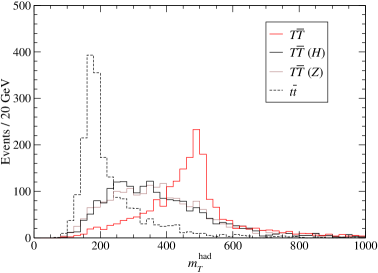
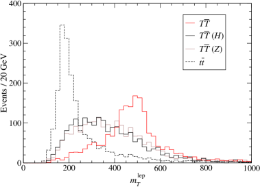
(a)	(b)
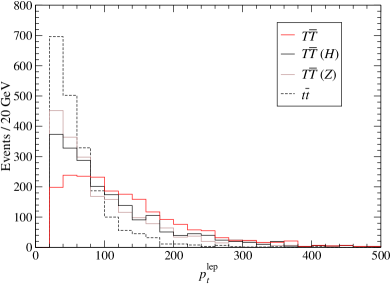
(c)

Figure 1: Reconstructed masses of the heavy quarks decaying hadronically (a) and semileptonically (b), and transverse momentum of the charged lepton (c), after pre-selection cuts.

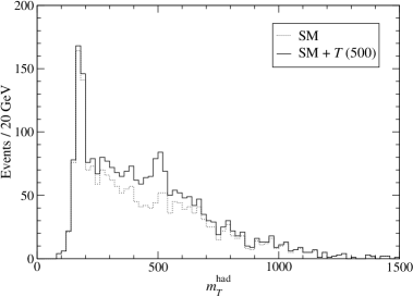
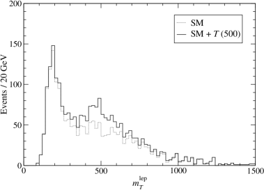
(a)	(b)

Figure 2: Reconstructed masses of the heavy quarks decaying hadronically (a) and semileptonically (b), after selection cuts. The dashed lines correspond to the SM predictions, while the full lines represent the SM plus a new 500 GeV quark.

The mass distributions after selection cuts of the SM background and background plus signal are shown in Fig. 2. The number of events $N_{\mathrm{cut}}$ corresponding to each process can be read in Table 2. The second column displays the numbers of events in the peak region, defined as

$$300~{}\mathrm{GeV}\leq m_{T}^{\mathrm{had}}\leq 660~{}\mathrm{GeV}\;,\quad 300~{}\mathrm{GeV}\leq m_{T}^{\mathrm{lep}}\leq 660~{}\mathrm{GeV}\,.$$ (3)

In this region, the statistical significance of the signals is $\mathcal{S}_{0}\equiv S/\sqrt{B}=10.94$ or, if we include a 5% background normalisation uncertainty, $\mathcal{S}_{5}\equiv S/\sqrt{B+(0.05B)^{2}}=7.69$. Discovery of the new quark would be possible with 2.1 fb^-1 of luminosity (2.8 fb^-1 if we include the background uncertainty).

Process	$N_{\mathrm{cut}}$	$N_{\mathrm{peak}}$
$T\bar{T}$ (500)	201.7	135.5
$T\bar{T}$ (500, $H$)	139.4	59.5
$T\bar{T}$ (500, $Z$)	58.5	26.5
$t\bar{t}$	1609	300
$Wb\bar{b}jj$	287	81
$Zb\bar{b}jj$	39	13
$t\bar{b}j$	70	16

Table 2: Number of events $N_{\mathrm{cut}}$ passing the selection criteria and number of events $N_{\mathrm{peak}}$ passing the selection cuts which are in the peak regions.

4 Results for $\boldsymbol{m_{T}=1}$ TeV

The simulation in this case is done for 300 fb^-1 in the high luminosity LHC run. The $b$ tagging efficiency assumed is of 50%. The reconstructed masses of the two quarks are shown in Fig. 3 (a) and (b). For the $H$ and $Z$ signals the events are spread over a wide range of $m_{T}^{\mathrm{had}}$ and $m_{T}^{\mathrm{lep}}$ values, and for this $T$ mass a smaller fraction of events is in the vicinity of $m_{T}$. The charged lepton transverse momentum is plotted in Fig. 3 (c). For a heavy quark mass of 1 TeV, the lepton momentum distribution from $T\to W^{+}b\to\ell^{+}\nu b$ has a very long tail. Requiring $p_{t}^{\mathrm{lep}}\geq 200$ GeV eliminates 98% of the $t\bar{t}$ background, while keeping 51% of the $W^{+}bW^{-}\bar{b}$ signal. Our selection criteria are in this case

$$p_{t}^{j,\mathrm{max}}\geq 400~{}\mathrm{GeV}\,,\quad p_{t}^{b,\mathrm{max}}\geq 300~{}\mathrm{GeV}\,,$$

$$p_{t}^{\mathrm{lep}}\geq 200~{}\mathrm{GeV}\,,\quad 50~{}\mathrm{GeV}\leq p_{t}\!\!\!\!\!\!\!\!\not\,\,\,\,\,\,\leq 400~{}\mathrm{GeV}\,,$$

$$H_{t}\geq 1800~{}\mathrm{GeV}\,.$$ (4)

The mass distributions after these cuts are shown in Fig. 4. The number of events $N_{\mathrm{cut}}$ corresponding to each process can be read in the first column of Table 3, and the number of events in the peak region

$$800~{}\mathrm{GeV}\leq m_{T}^{\mathrm{had}}\leq 1200~{}\mathrm{GeV}\;,\quad 800~{}\mathrm{GeV}\leq m_{T}^{\mathrm{lep}}\leq 1200~{}\mathrm{GeV}$$ (5)

in the second column. The statistical significance of the $T$ signal is $\mathcal{S}_{0}=9.09$, $\mathcal{S}_{5}=8.82$. The luminosity required to discover a 1 TeV quark in pair production is 90 fb^-1.

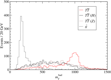
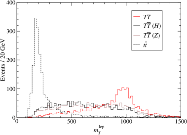
(a)	(b)
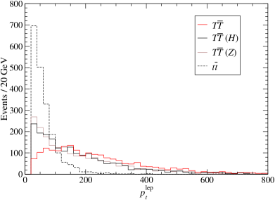
(c)

Figure 3: Reconstructed masses of the heavy quarks decaying hadronically (a) and semileptonically (b), and transverse momentum of the charged lepton (c), after pre-selection cuts.

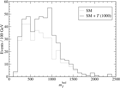
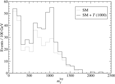
(a)	(b)

Figure 4: Reconstructed masses of the heavy quarks decaying hadronically (a) and semileptonically (b), after selection cuts. The dashed lines correspond to the SM predictions, while the full lines represent the SM plus a new 1 TeV quark.

Process	$N_{\mathrm{cut}}$	$N_{\mathrm{peak}}$
$T\bar{T}$ (1000)	58.2	33.5
$T\bar{T}$ (1000, $H$)	39.6	7.8
$T\bar{T}$ (1000, $Z$)	21.0	5.1
$t\bar{t}$	208	10
$Wb\bar{b}jj$	132	15
$Zb\bar{b}jj$	19	1
$t\bar{b}j$	3	0

Table 3: Number of events $N_{\mathrm{cut}}$ passing the selection criteria and number of events $N_{\mathrm{peak}}$ passing the selection cuts which are in the peak regions.

5 Discussion

We can compare the results obtained here with those from $T\bar{T}\to W^{+}b\,H\bar{t},HtW^{-}\bar{b}$ decays in the final state $\ell\nu bbbbjj$, requiring four $b$ tags [14]. For $m_{T}=500$ GeV and 10 fb^-1 of luminosity, the latter channel has a similar sensitivity, $\mathcal{S}_{0}=10.86$ , $\mathcal{S}_{5}=10.13$, which is achieved with a good $b$ tagging performance, which suppresses the dangerous $t\bar{t}jj$ and $W+~{}$ jets backgrounds. We also note that the $\ell\nu bbbbjj$ channel has a slightly larger branching ratio than $\ell\nu bbjj$ final states. Combining both channels, a 500 GeV singlet can be discovered already with a luminosity of 1.2 fb^-1.

For $m_{T}=1$ TeV the situation is rather different. The $T\bar{T}\to W^{+}bW^{-}\bar{b}$ signal is characterised by the presence of a very energetic charged lepton, not only due to the higher energy available in $T$ decays but also because of spin effects. Let us analyse these issues more in detail. For $m_{T}=1$ TeV, the fraction of $W$ bosons with negative helicity produced in $T$ decays is $f_{-}=0.013$, compared to $f_{-}=0.297$ for the top quark, and then the charged lepton from $W$ decay is produced more towards the $W$ flight direction. (The fraction of $W$ bosons with positive helicity $f_{+}$ is negligible in both cases due to angular momentum conservation; the zero helicity fraction is then $f_{0}\simeq 1-f_{-}$.) This is reflected in the charged lepton energy distribution in the rest frame of the decaying quark, which is [26]

$$\frac{1}{\Gamma}\frac{d\Gamma}{dE_{\ell}} = \frac{1}{(E_{\ell}^{\text{max}}-E_{\ell}^{\text{min}})^{3}}\left[3(E_{\ell}-E_{\ell}^{\text{min}})^{2}\,f_{+}+3(E_{\ell}^{\text{max}}-E_{\ell})^{2}\,f_{-}\right.$$ (6)

$$\left.+6(E_{\ell}^{\text{max}}-E_{\ell})(E_{\ell}-E_{\ell}^{\text{min}})\,f_{0}\right]\,,$$

with $E_{\ell}^{\text{max}}$, $E_{\ell}^{\text{min}}$ the maximum and minimum charged lepton energies in the rest frame of the decaying quark ($E_{\ell}^{\text{min}}=18.5$ GeV, $E_{\ell}^{\text{max}}=87.4$ GeV for $t$; $E_{\ell}^{\text{min}}=3.2$ GeV, $E_{\ell}^{\text{max}}=500$ GeV for $T$). The normalised energy distributions of the charged lepton from $t$ and $T$ semileptonic decays are plotted in Fig. 5, where we have scaled both axes to fully appreciate the spin effect. The different shape of the curves is reflected in the $p_{t}^{\mathrm{lep}}$ distributions in Fig. 3.

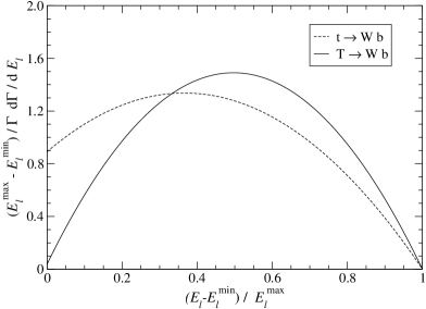
Figure 5: Normalised energy distributions of the charged lepton from $t$ and $T$ semileptonic decays.

For $m_{T}=1$ TeV, the requirement of high $p_{t}^{\mathrm{lep}}$ can be used to reduce backgrounds significantly in the $T\bar{T}\to W^{+}bW^{-}\bar{b}$ mode but not in $T\bar{T}\to W^{+}b\,H\bar{t},HtW^{-}\bar{b}$ decays, where half of the events have a charged lepton coming from a top (anti)quark. (By the same reason, the $H$ and $Z$ contributions studied in this work are suppressed.) This might be partly compensated with a good $b$ tagging efficiency to reject backgrounds, but at the high luminosity LHC run, where masses of the order of 1 TeV can be investigated, light jet and charm rejection is degraded. A preliminary analysis has shown that for $m_{T}=1$ TeV and 300 fb^-1 of luminosity the significance achieved in the $\ell\nu bbbbjj$ channel is $S/\sqrt{B}\lesssim 3$, three times smaller than in the $\ell\nu bbjj$ mode analysed here.

- [1] F. del Aguila and J. Santiago, JHEP 0203 (2002) 010; see also F. del Aguila, M. Perez-Victoria and J. Santiago, hep-ph/0305119; Acta Phys. Polon. B 34 (2003) 5511
- [2] V. D. Barger, M. S. Berger and R. J. N. Phillips, Phys. Rev. D 52 (1995) 1663
- [3] P. H. Frampton, P. Q. Hung and M. Sher, Phys. Rept. 330 (2000) 263
- [4] N. Arkani-Hamed, A. G. Cohen and H. Georgi, Phys. Lett. B 513 (2001) 232
- [5] F. del Aguila and M. J. Bowick, Nucl. Phys. B 224 (1983) 107
- [6] T. Morozumi, T. Satou, M. N. Rebelo and M. Tanimoto, Phys. Lett. B 410 (1997) 233; Y. Kiyo, T. Morozumi, P. Parada, M. N. Rebelo and M. Tanimoto, Prog. Theor. Phys. 101 (1999) 671
- [7] F. del Aguila, J. A. Aguilar-Saavedra and R. Miquel, Phys. Rev. Lett. 82 (1999) 1628
- [8] J. A. Aguilar-Saavedra, Phys. Rev. D 67 (2003) 035003 [Erratum-ibid. D 69 (2004) 099901]
- [9] G. C. Branco, P. A. Parada and M. N. Rebelo, Phys. Rev. D 52 (1995) 4217
- [10] G. C. Branco, T. Morozumi, P. A. Parada and M. N. Rebelo, Phys. Rev. D 48 (1993) 1167
- [11] J. A. Aguilar-Saavedra, F. J. Botella, G. C. Branco and M. Nebot, Nucl. Phys. B 706 (2005) 204
- [12] F. del Aguila, G. L. Kane and M. Quiros, Phys. Rev. Lett. 63 (1989) 942
- [13] F. del Aguila, L. Ametller, G. L. Kane and J. Vidal, Nucl. Phys. B 334 (1990) 1
- [14] J. A. Aguilar-Saavedra, hep-ph/0603200
- [15] T. Han, H. E. Logan, B. McElrath and L. T. Wang, Phys. Rev. D 67 (2003) 095004
- [16] F. del Aguila and R. Pittau, Acta Phys. Polon. B 35 (2004) 2767
- [17] G. Azuelos et al., Eur. Phys. J. C 39S2 (2005) 13
- [18] D. Costanzo, ATLAS note ATL-PHYS-2004-004
- [19] J. A. Aguilar-Saavedra, Phys. Lett. B 625 (2005) 234 [Erratum-ibid. B 633 (2006) 792]
- [20] E. Murayama, I. Watanabe and K. Hagiwara, KEK report 91-11, January 1992
- [21] M. L. Mangano, M. Moretti, F. Piccinini, R. Pittau and A. D. Polosa, JHEP 0307 (2003) 001; See also http://mlm.home.cern.ch/m/mlm/www/alpgen/
- [22] H. L. Lai et al. [CTEQ Collaboration], Eur. Phys. J. C 12 (2000) 375
- [23] T. Sjostrand, P. Eden, C. Friberg, L. Lonnblad, G. Miu, S. Mrenna and E. Norrbin, Comput. Phys. Commun. 135 (2001) 238
- [24] R. Barate et al. [ALEPH Collaboration], Phys. Rept. 294 (1998) 1
- [25] E. Richter-Was, D. Froidevaux and L. Poggioli, ATL-PHYS-98-131
- [26] J. A. Aguilar–Saavedra, J. Carvalho, N. Castro, A. Onofre and F. Veloso, in preparation