Abstract

We discuss the higher Fock state ($q\bar{q}g$) contributions to the nonzero value of the pion GPD at the crossover point $x=\zeta$ between the DGLAP and ERBL regions. Using the phenomenological light-front constituent quark model, we confirm that the higher Fock state contributions indeed give a nonzero value of the GPD at the crossover point. Iterating the light-front quark model wavefunction of the lowest $q\bar{q}$ Fock state with the Bethe-Salpeter kernel corresponding to the one-gluon-exchange, we include all possible time-ordered $q\bar{q}g$ Fock state contributions and obtain the pion GPD satisfying necessary sum rules and continuity conditions.

PACS number(s): 13.40.Gp, 13.60.Fz, 14.40.Aq

I Introduction

The Compton scattering provides a unique tool for studying hadronic structure. In distinction to hadronic form factors, the Compton amplitude probes the hadrons through a coupling of two electromagnetic currents, and thus provides a wealth of additional information. When the initial photon is highly virtual while the final one is real, one arrives at the kinematics of deeply virtual Compton scattering (DVCS), the process [1, 2] which was a subject of intensive theoretical analysis during the last decade. Within the perturbative Quantum ChromoDynamics (QCD), it was established [3, 1, 2, 4, 5] that the most important contribution to the amplitude of this exclusive process is given by the convolution of a hard quark propagator and a nonperturbative function describing long-distance dynamics which is now known as a “generalized parton distribution (GPD)” [3, 1, 2] (see [6, 7, 8] for recent detailed reviews). The GPDs serve as a generalization of the ordinary (forward) parton distributions and provide much more direct and sensitive information on the light-front (LF) wavefunctions of the target hadron than the hadron form factors. In particular, the momentum of the “probed quark” in GPDs is kept fixed at longitudinal momentum fraction $x$, while for the form factor it is integrated out (due to the nonlocal current operator $\bar{\psi}(0)\gamma^{\mu}\psi(z)$ for the GPDs in contrast to the local vertex $\bar{\psi}(0)\gamma^{\mu}\psi(0)$ for the form factor). Within the GPD approach, form factors are treated as just the lowest moments of the GPDs. Because of being generalized amplitudes, the GPDs always involve the nonvalence contributions due to the presence of the asymmetry between the longitudinal initial $P$ and final $P^{\prime}$ hadron momenta characterized by the “skewness” parameter $\zeta=(P-P^{\prime})^{+}/P^{+}$. The kinematic region where the longitudinal momentum fraction $x$ of the probed quark is greater than the skewness parameter $\zeta$ (i.e. $1>x>\zeta$) is called “DGLAP region” (the evolution pattern for GPDs there is similar to the DGLAP evolution [9, 10, 11] of ordinary parton distributions) while the remaining part $0<x<\zeta$ of the longitudinal momenta $0<x<\zeta$ is called “ERBL region” (GPDs in this case have ERBL-type evolution [12, 13] characteristic of meson distribution amplitudes). In the framework of LF dynamics, the DGLAP and ERBL regions have also been denoted as the valence and nonvalence regions, respectively, because the parton-number-changing nonvalence Fock-state contributions cannot be avoided for $0<x<\zeta$ while only the parton-number-conserving valence Fock-state contributions are needed for $1>x>\zeta$. Thus, it has been a great challenge to calculate the nonvalence contributions to the GPDs in the framework of LF quantization.

Although many recent theoretical endeavors [14, 15, 16, 17, 18, 19, 20] have been made in describing the GPDs in terms of LF wavefunctions, the results have not yet been satisfactory enough for practical calculations. In Refs. [15] and [16], the nonvalence contributions to the GPDs have been rewritten in terms of LF wavefunctions with different parton configurations. However, the representation given in Refs. [15] and [16] requires to find all the higher Fock-state wavefunctions while there has been relatively little progress in computing the basic wavefunctions of hadrons from first principles. In Refs. [17] and [18], the GPDs were expressed in terms of LF wavefunctions, but only within toy models such as the ’t Hooft model of $(1+1)$-dimensional QCD [17] and the scalar Wick-Cutkosky model [18]. While these toy model analyses are helpful to gain physical insight on the properties of the GPDs (especially, the time reversal invariance, the continuity at the crossover between the DGLAP and ERBL regions, and the sum rule constrained by the electromagnetic form factor), the real $(3+1)$-dimensional QCD motivates us to come up with a more realistic model for the application to the analysis of GPDs.

In an effort toward this direction, one of us (C. Ji) presented an effective treatment of handling the nonvalence contributions to the GPDs of the pion [19, 20] using the LF constituent quark model (LFQM), which has been phenomenologically quite successful in describing the space-like form factors for the electromagnetic and radiative decays of pseudoscalar and vector mesons [21, 22, 23] and the time-like weak form factors for exclusive semileptonic and rare decays of pseudoscalar mesons [24, 25, 26]. Our effective treatment of handling the nonvalence contributions is based on the covariant Bethe-Salpeter (BS) approach formulated in the LF quantization [24] which we call LFBS approach. It has been previously applied to the exclusive semileptonic and rare decays of pseudoscalar mesons [25, 26] providing reasonable results compared to the data. The projection of the four-dimensional two-body BS equations at the light-front hypersurface has also been discussed in Ref. [27] and the problem of constructing gauge invariant current in terms of LF bound-state wavefunctions has been handled in Ref. [28]

In Ref.[19], an artifact of discontinuity at $x=\zeta$ between valence and nonvalence parts of the GPD had occurred but it was later cured in the framework of the same LFBS approach by taking into account both the vertices of the meson and of the gauge boson [20]. Due to the consistent treatment of the vertices, the continuity of the GPD at the crossover point $x=\zeta$ was secured. However, the value of the GPD at the crossover point vanished due to the end-point behavior of the LF wavefunctions of meson and gauge boson. In Ref.[20], it was noted that it may be possible to avoid this effect of GPDs’ vanishing at the crossover point by considering contributions of the higher Fock states in the DVCS amplitude. In this work, we examine if the GPD value at the crossover point is indeed nonzero including the higher Fock state corrections. This investigation is particularly important because the recent measurement of the single spin asymmetry (SSA) at HERMES [29] and CLAS [30] indicate that the value of GPD at the crossover point does not vanish for the proton. Although the internal structure of the pion is rather different from that of the proton, the issue of GPDs’ vanishing or not vanishing at the crossover point is common to all bound states. Thus, establishing the link between the nonzero value of GPDs at the crossover point and the higher Fock-state contributions is a result applicable for both hadrons.

Working in the same LFBS framework, we will consider in addition to the pion LF wavefunction the contribution from the higher Fock components of $q{\bar{q}}g$. We first follow the analysis of the higher Fock state contributions presented in Ref.[18] and find that the analysis of Ref.[18] is correct only if one uses the exact solution of the BS equation. Later, the authors of Ref. [18] investigated the current matrix elements in the LFBS formalism discussing the replacement of non-wavefunction vertices [31] and applying it to GPDs [32]. Using a simple model, they obtained expressions for GPDs that are continuous and noted that the nonvanishing of GPDs at the crossover point is tied to higher Fock components. Our work develops the QCD application to the continuous and nonvanishing GPDs at the crossover point. We present explicit numerical results in QCD. For a model LF wavefunction we show that one shall retain all contributions including the ones that ideally could be absorbed into the LF wavefunction through the Bethe-Salpeter equation. This suggests a necessary improvement of the model wavefunctions by iterating them with the BS kernel.

This work is organized as follows. In Section II, we go over briefly the essentials of the LF kinematics of the DVCS. In Section III, we review previous advances in LFBS effective treatment of the pion GPD. Then, in Section IV, we extend LFBS approach to include $q{\bar{q}}g$ Fock states and present the details of our calculations and numerical results including the application of the prescription given in Ref.[18]. Concluding remarks follow in Section IV. The pole assignment for the Cauchy integration and the comments on the organization of the numerical calculations are presented in Appendices A and B, respectively.

II Light-Front Kinematics of the Deeply Virtual Compton Scattering

We begin with the kinematics of the virtual Compton scattering off the pion (see Fig.1)

$$\gamma^{*}(q)+\pi(P)\to\gamma(q^{\prime})+\pi(P^{\prime}).$$ (1)

FIG. 1.: Handbag diagrams that give the dominant contribution to Compton scattering in the deeply virtual regime. The lower “soft” part consists of a hadronic matrix element which is parametrized by generalized parton distribution functions.

The initial (final) hadron state is characterized by the momentum $P$ $(P^{\prime})$, and the incoming virtual (space-like) and outgoing real photons are characterized by the momenta $q$ and $q^{\prime}$, respectively. In this work, we use the LF-metric $V\cdot V=V^{+}V^{-}-{\bf V}_{\perp}^{2}$. Defining the four momentum transfer $\Delta=P-P^{\prime}$, one has

$$P=\biggl{(}P^{+},M^{2}/P^{+},0_{\perp}\biggr{)}\ \ ,\ \ P^{\prime}=\biggl{(}(1-\zeta)P^{+},(M^{2}+{\bf\Delta}^{2}_{\perp})/(1-\zeta)P^{+},-{\bf\Delta}_{\perp}\biggr{)}\ ,$$

and

$$\Delta=P-P^{\prime}=(\zeta P^{+},(\Delta^{2}+{\bf\Delta}^{2}_{\perp})/\zeta P^{+},{\bf\Delta}_{\perp})\ ,$$

where $M$ is the mass of the pion and $\zeta=\Delta^{+}/P^{+}$ is the skewness parameter describing the longitudinal momentum asymmetry of GPDs. The squared momentum transfer is given by

$$t=\Delta^{2}=2P\cdot\Delta=-\frac{\zeta^{2}M^{2}+{\bf\Delta}^{2}_{\perp}}{1-\zeta}\ .$$ (2)

Since ${\bf\Delta}^{2}_{\perp}\geq 0$ at given $\zeta$, the value of $-t$ is constrained from below: $-t>-t_{\min}=\zeta^{2}M^{2}/(1-\zeta)$.

As shown in Fig.1, the parton emitted by the pion has the momentum $k$, and the absorbed parton has the momentum $k^{\prime}=k-\Delta$. Just like in the case of space-like form factors, we may choose a frame where the incident space-like photon has zero plus component, $q^{+}=0$, so that

$$\begin{array}[]{c}q=\left(0,{({\bf q}_{\perp}+{\bf\Delta}_{\perp})^{2}}/{\zeta P^{+}}+(\zeta M^{2}+{\bf\Delta}^{2}_{\perp})/{(1-\zeta)P^{+}},{\bf q}_{\perp}\right)\ \ ,\ \ q^{\prime}=\left(\zeta P^{+},{({\bf q}_{\perp}+{\bf\Delta}_{\perp})^{2}}/{\zeta P^{+}},{\bf q}_{\perp}+{\bf\Delta}_{\perp}\right).\end{array}$$ (3)

In DVCS, where $Q^{2}=-q^{2}\gg M^{2}$, and $Q^{2}\gg-t$ is large, $\zeta$ plays the role of the Bjorken variable, i.e. $Q^{2}/(2P\cdot q)=\zeta$. For a fixed value of $-t$, the allowed range of $\zeta$ is given by

$$0\leq\zeta\leq\frac{(-t)}{2M^{2}}\,\biggl{(}\sqrt{1+\frac{4M^{2}}{(-t)}}-1\biggr{)}.$$ (4)

In the leading twist, ignoring interactions at the quark-gauge-boson (photon in this case) vertex, the dominant contribution to the Compton scattering amplitude in the deeply virtual region is given by

$$M^{\mu\nu}=M^{\mu\nu}_{s}+M^{\mu\nu}_{u}\ ,$$ (5)

i.e. the sum of the $s$-channel amplitude $M^{\mu\nu}_{s}$ and the $u$-channel amplitude $M^{\mu\nu}_{u}$ shown in Fig.1. The $s$-channel amplitude is given by

$$M^{\mu\nu}_{s} = -iN_{c}e^{2}_{q}\int\frac{d^{4}k}{(2\pi)^{4}}{\rm Tr}\,[\gamma_{5}(\not\!k+m)\gamma^{\mu}(\not\!k+\not\!q+m)\gamma^{\nu}(\not\!k-\not\!\Delta+m)\gamma_{5}(-\not\!P+\not\!k+m)]$$ (6)

$$\times \frac{H_{\rm cov}(k,P)H^{\prime}_{\rm cov}(k-\Delta,P-\Delta)}{[k^{2}-m^{2}+i\varepsilon][(k+q)^{2}-m^{2}+i\varepsilon][(k-\Delta)^{2}-m^{2}+i\varepsilon][(P-k)^{2}-m^{2}+i\varepsilon]},$$ (7)

where $N_{c}$ is the color factor and $H_{\rm cov}(k,P)$ $[H^{\prime}_{\rm cov}(k-\Delta,P-\Delta)]$ is the covariant initial [final] state meson-quark vertex function that satisfies the BS equation. As usual in the LFBS formalism, we assume that the covariant vertex function $H_{\rm cov}(k)$ does not alter the $k^{-}$ pole structure in Eq. (6). The $u$-channel amplitude can be easily obtained by $M^{\mu\nu}_{u}=M^{\mu\nu}_{s}(q\to-q^{\prime})$.

The effective gauge-boson vertex is depicted in Fig.2 as a reduction from the Compton scattering amplitude of the virtual photon given by

$$(-ie_{q})^{2}\left(\frac{\not\!\epsilon i(\not\!q+\not\!k+m)\not\!\epsilon^{\prime}}{(q+k)^{2}-m^{2}+i\varepsilon}+\frac{\not\!\epsilon^{\prime}i(-\not\!q^{\prime}+\not\!k+m)\not\!\epsilon}{(k-q^{\prime})^{2}-m^{2}+i\varepsilon}\right)\ .$$ (8)

FIG. 2.: Effective vertex

In the deep inelastic limit, we may neglect $\not\!k$ along with any 4-products not involving $q$ in the trace of the numerator (note that for circularly polarized photons also $q\cdot\epsilon$ and $q\cdot\epsilon^{\prime}$ can be neglected), i.e.

$$q^{2},q\cdot a\gg a\cdot b,m^{2}{\hbox{, }}\epsilon\cdot q,\epsilon^{\prime}\cdot q.$$ (9)

Then the amplitude (8) can be rewritten as

$$-ie_{q}^{2}\left(\frac{-\not\!q\not\!\epsilon\not\!\epsilon^{\prime}}{(q+k)^{2}-m^{2}+i\varepsilon}+\frac{\not\!q^{\prime}\not\!\epsilon^{\prime}\not\!\epsilon}{(k-q^{\prime})^{2}-m^{2}+i\varepsilon}\right)\,.$$ (10)

Furthermore, $\not\!\epsilon\not\!\epsilon^{\prime}$ can be written as $\epsilon\cdot\epsilon^{\prime}+i\sigma^{\mu\nu}\epsilon_{\mu}\epsilon^{\prime}_{\nu}$, where $\sigma^{\mu\nu}=\frac{1}{2i}[\gamma^{\mu},\gamma^{\nu}]$. The axial term can be neglected because it vanishes after integration over ${\bf k}_{\perp}$. Thus, for the reduced vertex we obtain

$$-ie_{q}^{2}(-\epsilon\cdot\epsilon^{\prime})\not\!q\left(\frac{1}{(q+k)^{2}-m^{2}+i\varepsilon}-\frac{1}{(k-q^{\prime})^{2}-m^{2}+i\varepsilon}\right)\sim$$ (11)

$$-ie_{q}^{2}(-g^{\mu\nu})\not\!q\left(\frac{1}{(q+k)^{2}-m^{2}+i\varepsilon}-\frac{1}{(k-q^{\prime})^{2}-m^{2}+i\varepsilon}\right)\,.$$ (12)

The denominators can be further simplified by

$$\left(\frac{1}{(q+k)^{2}-m^{2}+i\varepsilon}-\frac{1}{(k-q^{\prime})^{2}-m^{2}+i\varepsilon}\right)\sim\frac{1}{P^{+}q^{-}}\left(\frac{1}{x-\zeta+i\varepsilon}+\frac{1}{x-i\varepsilon}\right)\ .$$ (13)

Adding $s$- and $u$-channel amplitudes, we obtain the Compton scattering amplitude in DVCS limit as follows

$$M^{IJ}=\epsilon^{I}_{\mu}\epsilon^{*J}_{\nu}M^{\mu\nu} = -\frac{iN_{c}}{2P^{+}}e^{2}_{q}\int\frac{d^{4}k}{(2\pi)^{4}}\biggl{(}\frac{1}{x-\zeta+i\varepsilon}+\frac{1}{x-i\varepsilon}\biggr{)}H_{\rm cov}(k,P)H^{\prime}_{\rm cov}(k-\Delta,P-\Delta)$$ (14)

$$\times \frac{{\rm Tr}\,[\gamma_{5}(\not\!k+m)\not\!\epsilon^{I}\gamma^{+}\not\!\epsilon^{*J}(\not\!k-\not\!\Delta+m)\gamma_{5}(-\not\!P+\not\!k+m)]}{[k^{2}-m^{2}+i\varepsilon][(k-\Delta)^{2}-m^{2}+i\varepsilon][(P-k)^{2}-m^{2}+i\varepsilon]}.$$ (15)

For circularly polarized ($\epsilon^{+}=0$) initial and final photons($I,J$ are $\uparrow$ or $\downarrow$), we obtain from Eq. (14)

$$\not\!\epsilon^{I}\gamma^{+}\not\!\epsilon^{*J}=(\epsilon^{I}_{\perp}\cdot\epsilon^{*J}_{\perp})\gamma^{+}+i(\epsilon^{I}_{\perp}\times\epsilon^{*J}_{\perp})_{3}\gamma^{+}\gamma_{5}.$$ (16)

Equation (16) reduces to $\gamma^{+}(1\pm\gamma_{5})$ for the parallel helicities (i.e. $+$ for $\uparrow\uparrow$ and $-$ for $\downarrow\downarrow$) and zero otherwise. Since the axial current $\gamma^{+}\gamma_{5}$ does not contribute to the integral, i.e. $\sim({\bf k}_{\perp}\times{\bf\Delta}_{\perp})$ after the trace calculation, this term can be dropped.

Thus, the DVCS amplitude (i.e. photon helicity amplitude) can be rewritten as the factorized form of hard and soft amplitudes

$$M^{\uparrow\uparrow}(P,q,P^{\prime})=M^{\downarrow\downarrow}(P,q,P^{\prime})=-e^{2}_{q}\int\;dx\biggl{(}\frac{1}{x-\zeta+i\varepsilon}+\frac{1}{x-i\varepsilon}\biggr{)}{\cal F}_{\pi}(\zeta,x,t),$$ (17)

where

$${\cal F}_{\pi}(\zeta,x,t)= = \frac{iN_{c}}{2}\int\frac{dk^{-}d^{2}{\bf k}_{\perp}}{2(2\pi)^{4}}H_{\rm cov}(k,P)H^{\prime}_{\rm cov}(k-\Delta,P-\Delta)$$ (18)

$$\times \frac{{\rm Tr}\,[\gamma_{5}(\not\!k+m)\gamma^{+}(\not\!k-\not\!\Delta+m)\gamma_{5}(-\not\!P+\not\!k+m)]}{[k^{2}-m^{2}+i\varepsilon][(k-\Delta)^{2}-m^{2}+i\varepsilon][(P-k)^{2}-m^{2}+i\varepsilon]}.$$ (19)

The function ${\cal F}_{\pi}(\zeta,x,t)$ is the “generalized parton distribution” and it manifests characteristics of the ordinary(forward) quark distribution in the limits $\zeta\to 0$ and $t\to 0$. On the other hand, the first moment of ${\cal F}_{\pi}(\zeta,x,t)$ is related to the form factor by the following sum rule [1, 2]:

$$\int^{1}_{0}{dx}\,{\cal F}_{\pi}(\zeta,x,t)=(1-{\zeta}/{2})\,F_{\pi}(t).$$ (20)

In general, the polynomiality conditions for the moments of the GPDs[33, 34] defined by

$$\int^{1}_{0}dx\,x^{n-1}{\cal F}_{\pi}(\zeta,x,t)=(1-{\zeta}/{2})\,F_{n}(\zeta,t)$$ (21)

require that the highest power of $\zeta$ in the polynomial expression of $F_{n}(\zeta,t)$ should not be larger than $n$. These polynomiality conditions are fundamental properties of the GPDs which follow from the Lorentz invariance. The positivity property of the GPDs, following from positivity of the density matrix [35], has been discussed analyzing the double distributions (DD) [36]. While such conditions as sum rules and polynomiality are more easily satisfied by the DD-based models for the GPDs, it has been noted[36] that the positivity constraints are more transparent in the framework based on the LF wavefunction.

An important feature of the DVCS amplitude given by Eq. (17) is that it depends only on the skewness parameter $\zeta=Q^{2}/(2P\cdot q)$ for large $Q^{2}$ and fixed $|t|(\leq Q^{2})$. This property of the exclusive DVCS amplitude is similar to the Bjorken scaling for the structure functions of the inclusive deep inelastic scattering (DIS) reaction. Moreover, for DVCS, the skewness parameter $\zeta$ coincides with the Bjorken variable $x_{Bj}$. Note also that, according to Eq. (17), the size of the imaginary part of the DVCS amplitude is proportional to ${\cal F}_{\pi}(\zeta,\zeta,t)$, i.e., to the value of the GPD at the crossover point $x=\zeta$. In its turn, the imaginary part of the DVCS amplitude determines the magnitude of the single spin asymmetry (SSA) [1] (see also [37, 38]) that can be measured through the scattering of longitudinally polarized electrons on an unpolarized target. The SSA measurements for the proton target have been reported by HERMES [29] and CLAS [30] collaborations, with the magnitude of the SSA definetely inconsistent with zero.

III Light Front Bethe-Salpeter approach for the generalized parton distributions.

Let us now consider an explicit form of the GPD defined by Eq. (18) in the framework of Light-Front dynamics. Corresponding to the $x<\zeta$ and $x>\zeta$ regions of the covariant amplitude (see Fig.3), the Cauchy integration over $k^{-}$ in Eq. (18) has nonzero contribution coming either from the residue of the pole at $(P-k)^{2}=m^{2}$ in the valence region $x>\zeta$ or from the pole at $k^{2}=m^{2}$ in the non-valence region $x<\zeta$.

FIG. 3.: Covariant amplitude with reduced photon vertex for pion GPD (left) and its non-valence $x<\zeta$ part (right).

These two cases correspond to two different time-ordered LF diagrams which we will consider separately. In the region of $\zeta<x$ the residue is taken at the pole in upper half-plane $k^{-}$ relevant to $(P-k)^{2}=m^{2}$, i.e. $k^{-}=P^{-}-(P-k)^{-}_{\rm on}+i\epsilon=P^{-}-[{\bf k}^{2}_{\perp}+m^{2}]/(P-k)^{+}+i\epsilon$. Performing the Cauchy integration over $k^{-}$ in this region we find

$$k^{2}-m^{2}=k^{+}k^{-}-{\bf k}_{\perp}^{2}-m^{2}\rightarrow k^{+}(P^{-}-k^{-}_{\rm on}-(P-k)^{-}_{\rm on})=x\left(M^{2}-\frac{{\bf k}^{2}_{\perp}+m^{2}}{x(1-x)}\right)\ ,$$ (22)

$$(k-\Delta)^{2}-m^{2}\rightarrow(k-\Delta)^{+}(P^{-}-\Delta^{-}-(P-k)^{-}_{\rm on}-(k-\Delta)^{-}_{\rm on})=x^{\prime}\left(M^{2}-\frac{k^{\prime 2}_{\perp}+m^{2}}{x^{\prime}(1-x^{\prime})}\right)\ ,$$ (23)

where

$$x^{\prime}=\frac{x-\zeta}{1-\zeta}\ \ \text{ and }\ \ {\bf k^{\prime}}_{\perp}={\bf k}_{\perp}-{\bf\Delta}_{\perp}+x^{\prime}{\bf\Delta}_{\perp}$$ (24)

are the “internal” LF-momenta of the quark absorbed into the final pion state ($x^{\prime}$ evidently has the meaning of the plus-momentum of the absorbed quark measured in units of the final hadron plus-momentum). Thus, the Cauchy integration in Eq. (18) over $k^{-}$ gives

$${\cal F}^{\rm val}_{\pi}(\zeta,x,t)=\frac{N_{c}}{2P^{+}}\frac{1}{16\pi^{3}}\frac{1}{(1-x)xx^{\prime}}\int d^{2}{\bf k}_{\perp}\,\chi_{(2\to 2)}(x,{\bf k}_{\perp})\,S^{+}_{\rm val}\,\chi^{\prime}_{(2\to 2)}(x^{\prime},{\bf k}^{\prime}_{\perp}),$$ (25)

where

$$\chi_{(2\to 2)} = \frac{h_{LF}}{M^{2}-M^{2}_{0}}\ \ ,\ \ M^{2}_{0}=\frac{{\bf k}^{2}_{\perp}+m^{2}}{1-x}+\frac{{\bf k}^{2}_{\perp}+m^{2}}{x},$$ (26)

$$\chi^{\prime}_{(2\to 2)} = \frac{h^{\prime}_{LF}}{M^{2}-M^{\prime 2}_{0}}\ \ ,\ \ M^{\prime 2}_{0}=\frac{{\bf k^{\prime}}^{2}_{\perp}+m^{2}}{1-x^{\prime}}+\frac{{\bf k^{\prime}}^{2}_{\perp}+m^{2}}{x^{\prime}},$$ (27)

and $S^{+}_{\rm val}$ is the trace in Eq. (18) evaluated at the point $(P-k)^{2}=m^{2}$; i.e.

$$S^{+}_{\rm val}=\frac{4P^{+}}{1-x^{\prime}}\,({\bf k}_{\perp}\cdot{\bf k^{\prime}}_{\perp}+m^{2}).$$ (28)

The light-front vertex functions $h_{LF}$ and $h^{\prime}_{LF}$ can be related to the covariant $H_{\rm cov}$ and $H^{\prime}_{\rm cov}$ vertex functions and then to LF wavefunctions, e.g., via instantaneous approximation following [18]. Here, following [20], we identify the LF wavefunction in $\chi_{(2\to 2)}$ as

$$\chi_{(2\to 2)}(x,{\bf k}_{\perp})=\sqrt{\frac{8\pi^{3}}{N_{c}}}\sqrt{\frac{\partial k_{z}}{\partial x}}\,\frac{[x(1-x)]^{1/2}}{M_{0}}\,\phi(x,{\bf k}_{\perp}),$$ (29)

where the Jacobian of the transformation ${\bf k}=(k_{z},{\bf k}_{\perp})\to(x,{\bf k}_{\perp})$ is obtained using $\partial k_{z}/\partial x=M_{0}/[4x(1-x)]$ with $M_{0}=\sqrt{\frac{{\bf k}_{\perp}^{2}+m^{2}}{x(1-x)}}$, and the radial wavefunction is given by

$$\phi(x,{\bf k}_{\perp}^{2})=\chi\,\sqrt{\frac{1}{\pi^{3/2}\beta^{3}}}\exp\left\{\frac{M^{2}-({\bf k}^{2}_{\perp}+m^{2})/(x(1-x))}{8\beta^{2}}\right\}.$$ (30)

The normalization factor $\chi=1$ is introduced for future convenience and is fixed by the normalization of the pion form-factor $F_{\pi}(t=0)=1$. After some simplifications, Eq. (29) can be written as

$$\chi_{(2\to 2)}(x,{\bf k}_{\perp})=\sqrt{\frac{2\pi^{3}}{N_{c}}}\frac{1}{\sqrt{M_{0}}}\phi(x,{\bf k}_{\perp}).$$ (31)

Substituting Eq. (29) into Eq. (25), we obtain the valence part of the pion GPD:

$${\cal F}^{\rm val}_{\pi}(\zeta,x,t) = \int d^{2}{\bf k}_{\perp}\sqrt{\frac{\partial k^{\prime}_{z}}{\partial x^{\prime}}}\sqrt{\frac{\partial k_{z}}{\partial x}}\phi(x^{\prime},{\bf k^{\prime}}_{\perp})\phi(x,{\bf k}_{\perp})\frac{({\bf k}_{\perp}\cdot{\bf k^{\prime}}_{\perp}+m^{2})}{\sqrt{{\bf k}^{2}_{\perp}+m^{2}}\sqrt{{\bf k^{\prime}}^{2}_{\perp}+m^{2}}}.$$ (32)

In the region of $x<\zeta$, the residue shall be taken at the pole $k^{2}=m^{2}$, i.e. $k^{-}=k^{-}_{\rm on}=[{\bf k}^{2}_{\perp}+m^{2}]/k^{+}-i\epsilon$, which is located in the lower half of the complex-$k^{-}$ plane. One can show that in this case

$$(P-k)^{2}-m^{2}\rightarrow(1-x)\left(M^{2}-\frac{{\bf k}^{2}_{\perp}+m^{2}}{x(1-x)}\right),$$ (33)

$$(k-\Delta)^{2}-m^{2}\rightarrow(1-x^{\prime\prime})\left(\Delta^{2}-\frac{{\bf k}_{\perp}^{\prime\prime 2}+m^{2}}{x^{\prime\prime}(1-x^{\prime\prime})}\right),$$ (34)

where

$$x^{\prime\prime}=x/\zeta{\hbox{ \ \ and \ \ }}{\bf k}^{\prime\prime}_{\perp}={\bf k}_{\perp}+x^{\prime\prime}{\bf\Delta}_{\perp}$$ (35)

are the “internal” momenta of the quark annihilating into the photon. The second line in Eq. (34) is related to a “gauge-boson-wavefunction” $\chi^{g}$ [19].

Then the non-valence part of GPD after the Cauchy integration in Eq. (18) can be written as

$${\cal F}^{\rm nonval}_{\pi}(\zeta,x,t)=\frac{N_{c}}{2P^{+}}\frac{1}{16\pi^{3}}\frac{1}{x(1-x)(1-x^{\prime\prime})}\int d^{2}{\bf k}_{\perp}\,\chi_{(2\to 2)}(x,{\bf k}_{\perp})S^{+}_{\rm nonval}\,\chi^{g}(x,{\bf k^{\prime\prime}}_{\perp})\,h^{\prime}_{LF},$$ (36)

where $\chi_{2\rightarrow 2}$ and $\chi^{g}$ are the pion and gauge-boson LF wavefunctions and the final state LF vertex function $h^{\prime}_{LF}$ is now kept explicitly. The trace term at $k^{2}=m^{2}$ ($S^{+}_{\rm nonval}$) is given by

$$S^{+}_{\rm nonval}=S^{+}_{\rm val}+\frac{4P^{+}}{1-x^{\prime}}x(1-x)x^{\prime}(M^{2}-M^{2}_{0}).$$ (37)

FIG. 4.: The difference in valence and non-valence LF vertex functions $h^{\prime val}_{LF}$ and $h^{\prime nv}_{LF}$.

Unlike in the valence part of GPD, the final state vertex $h^{\prime}_{LF}$ cannot be simply reduced to a LF wavefunction since it does not describe annihilation/creation of quark-antiquark pair out of the pion state. It corresponds to the decay of a quark into a quark and a pion state, or, equivalently the annihilation of a pion and a quark into a quark (see Fig.4). However, it is worth noting that $h^{\prime}_{LF}$ for valence and non-valence contribution essentially are the special case of the same object, namely, the covariant vertex function $H(k,P)$, in different kinematic regions. In particular, they obey the same BS equation and, in principle, can be deduced from the usual LF wavefunction by analytic continuation, as pointed out in Refs.[19, 20].

Specifically, following Ref.[19], the $\chi$-functions in LF CQM are given by the solutions of the BS equation [24, 39, 40]

$$(M^{2}-M^{2}_{0})\chi(x_{i},{\bf k}_{i\perp})$$ (38)

$$=\int[dy][d^{2}{\bf l}_{\perp}]\,{\cal K}(x_{i},{\bf k}_{i\perp};y_{j},{\bf l}_{j\perp})\,\chi(y_{j},{\bf l}_{j\perp}),$$ (39)

where ${\cal K}$ is the full BS kernel (which in principle includes all the higher Fock-state contributions) and $M^{2}_{0}=(m^{2}+{\bf k}^{2}_{\perp})/(1-x)-(m^{2}+{\bf k}^{2}_{\perp})/x$. Both valence and nonvalence BS amplitudes satisfy Eq. (38). For the usual BS amplitude, referred as the valence wavefunction, $x$ is greater than $\zeta$, while for the nonvalence BS amplitude $x$ is less than $\zeta$. We use the notation for these two solutions

$$\chi_{(2\to 2)} = \chi^{\rm val},$$ (40)

$$\chi_{(1\to 3)} = \chi^{\rm nonval}.$$ (41)

FIG. 5.: LF interpretation of the non-valence vertex ($1\rightarrow 3$ blob).

This notation is motivated by the relationship to the Fock state picture, in which the parton number before and after the kernel is interpreted for the nonvalence vertex as changing from 1 to 3. According to [19, 20], the nonvalence BS amplitude shall be expressed via the valence BS amplitude and the full BS kernel in the relevant kinematic domain as illustrated in Fig.5:

$$(M^{2}-M^{2}_{0})\chi_{(1\to 3)}(x_{i},{\bf k}_{i\perp})$$ (42)

$$=\int[dy][d^{2}{\bf l}_{\perp}]{\cal K}(x_{i},{\bf k}_{i\perp};y_{j},{\bf l}_{j\perp})\chi_{(2\to 2)}(y_{j},{\bf l}_{j\perp}).$$ (43)

In a sense, the BS kernel in this region can be viewed as the sum of all processes resulting in creation of a quark-antiquark pair from the initial single quark state. With this in mind, we write the non-valence part of GPD (see left diagram in Fig.6) as

$${\cal F}^{\rm nonval}_{\pi}(\zeta,x,t) = \frac{N_{c}}{2P^{+}}\frac{1}{16\pi^{3}}\frac{1}{x(1-x)(1-x^{\prime\prime})}\int d^{2}{\bf k}_{\perp}\chi_{(2\to 2)}(x,{\bf k}_{\perp})S^{+}_{\rm nonval}\chi^{g}(x,{\bf k^{\prime\prime}}_{\perp})$$ (44)

$$\times \int\frac{dy}{y(1-y)}\int d^{2}{\bf l}_{\perp}{\cal K}(x,{\bf k}_{\perp};y,{\bf l}_{\perp})\chi_{(2\to 2)}(y,{\bf l}_{\perp}).$$ (45)

FIG. 6.: Non-valence part of GPD interpretation in LF CQM.

It may be also noted that one should as well consider in this case the process in which quark-antiquark pair is created not by the spectator quark, but by the interacting quark (see right diagram in Fig.6). In Ref.[20], it was shown that this contribution can be reduced to the form of Eq. (44) with a simple modification of the kernel

$${\tilde{\cal K}}(x^{\prime},{\bf k^{\prime}}_{\perp};y^{\prime},{\bf l^{\prime}}_{\perp}) \equiv {\cal K}(x^{\prime},{\bf k^{\prime}}_{\perp};y^{\prime},{\bf l^{\prime}}_{\perp})\biggl{[}1-\frac{S^{+}_{\rm nonval}(y,{\bf l}_{\perp}){\tilde{\chi}}^{\rm i}_{b}(y,{\bf l}_{\perp})}{S^{+}_{\rm nonval}(x,{\bf k}_{\perp}){\tilde{\chi}}^{\rm i}_{a}(x,{\bf k}_{\perp})}\biggr{]},$$ (47)

where ${\tilde{\chi}}^{\rm i}_{a,b}$ denotes kinematic prefactors like $x(1-x)(1-x^{\prime\prime})$ etc. in the expressions corresponding to the diagrams shown in Fig.6.

Thus, we obtained the amplitude corresponding to the nonvalence contribution given by Eq. (36) in terms of ordinary light-front wavefunctions of hadron ($\chi_{(2\to 2)}$) and gauge-boson ($\chi^{g}$). This method, however, requires the knowledge of the full BS kernel ${\cal K}(x,{\bf k}_{\perp};y,{\bf l}_{\perp})$ which is in general dependent on the momenta connecting the one-body to three-body sectors, as depicted in Fig.5. While the relevant operator ${\cal K}$ in general involves all momenta $(x,{\bf k}_{\perp};y,{\bf l}_{\perp})$, the integral of ${\cal K}$ over $y$ and ${\bf l}_{\perp}$ in Eq. (44),

$$G_{\pi} \equiv \int^{1}_{0}\frac{dy^{\prime}}{y^{\prime}(1-y^{\prime})}\int d^{2}{\bf l}_{\perp}{\tilde{\cal K}}(x,{\bf k}_{\perp};y^{\prime},{\bf l^{\prime}}_{\perp})\chi_{(2\to 2)}(y^{\prime},{\bf l^{\prime}}_{\perp}),$$ (48)

depends only on $x$ and ${\bf k}_{\perp}$. In this work, we approximate $G_{\pi}$ as a constant (mean value). This approximation has been previously tested in the analyses of exclusive semileptonic decay processes [19, 20, 24] and proved to be a good approximation at least in small momentum transfer region. The pion GPD, calculated in this way, looks like in Fig.7.

FIG. 7.: The pion GPD at $\zeta=0.5$, $t=-0.5$ GeV² computed using LFBS approach.

Using the “effective” gauge-boson wavefunction in the non-valence region in the form

$$\phi^{g}({\bf k_{\perp}^{\prime\prime}}^{2})=\sqrt{\frac{1}{\pi^{3/2}\beta^{3}}}\exp\left[-\frac{{\bf k}^{\prime\prime 2}_{\perp}+m^{2}}{8\beta^{2}x^{\prime\prime}(1-x^{\prime\prime})}\right]\exp\left(\frac{\Delta^{2}}{8\beta^{2}}\right),$$ (49)

one can ensure the continuity between the valence and the nonvalence parts of the GPD by suppressing the non-valence contribution at $x^{\prime}=x^{\prime\prime}=0$ [20]. This cures the discontinuity found previously in Ref.[19] whose origin can be traced down to the difference in the treatment of the valence and non-valence LF vertex functions. More specifically, the discontinuity in Ref.[19] originated from the crude approximation for the LF nonvalence vertex $h^{\prime\rm nonval}_{LF}$. As discussed in the general form above, the nonvalence vertex $h^{\prime\rm nonval}_{LF}$ is an analytic continuation of $h^{\prime\rm val}_{LF}$ into nonvalence kinematic domain so that it should be continuously and smoothly connected with the latter at the boundary between the valence and the nonvalence kinematic regions. We experimented with different forms of such extensions for the non-valence vertex, satisfying condition of continuity at $x^{\prime}=0$. One such possibility, e.g., could be

$$h^{\prime\rm nonval}_{LF}\sim G_{\pi}\exp\left[\frac{{\bf k}_{\perp}^{2}+m^{2}}{8x\beta^{2}}\right],$$ (50)

which has structure similar to that of the LF wavefunction, goes to a constant when $x\ll-\frac{m^{2}}{\beta^{2}}$, and vanishes at $x\rightarrow-0$, thus guaranteeing the continuity with the valence LF wavefunction $h_{LF}^{\rm val}$. However, the resultant behavior of the GPD in the non-valence region depends significantly on the detailed form of the model assumed for the extension of LF wavefunction into the non-valence region. On the other hand, while the introduction of the model for the nonvalence vertex satisfying these requirements is nontrivial, the inclusion of the virtual processes at the gauge-boson vertex using Eq. (49) removes the discontinuity at $x=\zeta$, thus alleviating the above problem at the lowest approximation of LFBS approach. Such a treatment ensures the vanishing of the nonvalence contribution at the crossover and also removes the infrared singularity in the amplitude. It was further suggested [20] that the value of the GPD at the crossover point needs not be zero because the higher Fock states in LFBS approach may introduce a nonzero contribution at this point. In the following section we will consider this suggestion in more detail and show that, after inclusion of the $q{\bar{q}}g$ contribution into the DVCS amplitude, this value indeed is not zero.

IV Effect of the higher Fock states in the LFBS approach for the pion GPD.

Our primary goal in this section is to analyze how GPDs are affected by the higher LF Fock states, especially at or near the crossover point $x=\zeta$. While the LFBS treatment in Section III can be considered as computing GPD with 2-body Fock state contributions (upper diagram in Fig.8), here we are interested in the effect of the 3-body Fock states as depicted in the lower diagram in Fig.8. We concentrate specifically on the effect of the Fock states that include a gluon in addition to the constituent quarks in the DVCS amplitude. As suggested in Ref.[20], such contributions may result in a nonzero value at the crossover point of the GPD.

FIG. 8.: 2-body and 3-body contributions to pion GPD in LF.

Given that there had been relatively little progress in finding exact, or even model, form of the 3-body LF wavefunction in QCD from first principles, we choose to model it by relating 3-body Fock states to 2-body Fock states. As shown in Fig.9, we link 2-body states and 3-body states via a kernel including, in principle, all QCD processes which result in the production of one gluon along with the constituent quarks. Because of the complexity of such general kernel, in this work we limit ourselves to model it by the lowest-order simplest possible process shown by the right diagrams in Fig.9. Thus, when computing the GPD of the pion we will concentrate on the additional processes described by the covariant diagrams in Fig.10.

FIG. 9.: Relation between 2-body and 3-body Fock states (left) and an approximate relation for the kernel $K$ (right).

FIG. 10.: Next-Fock-State corrections to DVCS which we denote S1, S$1^{\prime}$ and S2 (left to right).

In Ref.[18], it was stated that, when considering processes such as those of Fig.10 in the LF dynamics, the time orderings when the additional gluon was exchanged entirely before (after) the photon emission should be omitted. This is because such contributions are related to initial (final) state interactions corresponding to iteration of the LF wavefunction with BS kernel. Due to BS equation, these exchanges can be entirely absorbed back into the LF wavefunction. For example, the first diagram in Fig.10, which we call S1, yields the three time-ordered contributions shown in Fig.11. According to Ref.[18], two left diagrams in Fig.11 are iterations of the LF wavefunction with the BS kernel in the one-gluon exchange approximation and, thus, should be absorbed into the LF vertex $h^{\rm val}_{LF}(y,{\bf k}_{\perp})$.

FIG. 11.: Different time ordered contributions for $x>\zeta$ in S1.

The only remaining contribution is the one where the gluon is present at the time of the photon emission, as shown by the right diagram in Fig.11. Using the LF-perturbation theory, we write this contribution as

$$\int\frac{dk^{+}d^{2}{\bf k}_{\perp}}{16\pi^{3}}\frac{dl^{+}d^{2}{\bf l}_{\perp}}{16\pi^{3}}fVh_{\rm in}(l;P)h_{\rm out}(k-\Delta;P-\Delta)$$ (51)

$$\times(-\zeta)\times{\rm Tr}\,[\gamma_{5}(\not\!l-\not\!P+m)\gamma^{\alpha}\overline{(\not\!k-\not\!P+m)}\gamma_{5}(\not\!k-\not\!\Delta+m)\not\!q\overline{(\not\!k+m)}\gamma_{\alpha}\overline{(\not\!l+m)}]$$ (52)

$$\times(-1)\times\left[l^{+}k^{+}(k-\Delta)^{+}(P-k)^{+}(P-l)^{+}(l-k)^{+}\right]^{-1}$$ (53)

$$\left\{[P^{-}-l^{-}_{\rm on}-(P-l)^{-}_{\rm on}][P^{-}-k^{-}_{\rm on}-(P-l)^{-}_{\rm on}-(l-k)^{-}_{\rm on}]\right.$$ (54)

$$\left.[P^{-}-\Delta^{-}-(k-\Delta)^{-}_{\rm on}-(P-l)^{-}_{\rm on}-(l-k)^{-}_{\rm on}][P^{-}-\Delta^{-}-(k-\Delta)^{-}_{\rm on}-(P-k)^{-}_{\rm on}]\right\}^{-1}\ .$$ (55)

By the overline we denote the parts which must be taken with the instantaneous contribution, i.e., with $k^{-}=P^{-}_{\rm tot}-\sum k^{-}_{i}$. This diagram contributes only to the region $\zeta<x<y$, and is zero otherwise. See Eq. (61) below for the definition of $f$ and $V$.

Similarly, for the final state interaction term S$1^{\prime}$, one can get three time-ordered diagrams in DGLAP region (modulo the instantaneous diagrams) shown in Fig.12. According to Ref.[18], out of these three, only the left diagram in Fig.12 should be kept. Using the LF-perturbation theory rules, we obtain that this contribution is given by

$$\int\frac{dk^{+}d^{2}{\bf k}_{\perp}}{16\pi^{3}}\frac{dl^{+}d^{2}{\bf l}_{\perp}}{16\pi^{3}}fVh_{\rm in}(k;P)h_{\rm out}(l-\Delta;P-\Delta)$$ (56)

$$\times(-\zeta Tr[\gamma_{5}\overline{(\not\!k-\not\!P+m)}\gamma^{\alpha}(\not\!l-\not\!P+m)\gamma_{5}\overline{(\not\!l-\not\!\Delta+m)}\gamma_{\alpha}\overline{(\not\!k-\not\!\Delta+m)}\not\!q(\not\!k+m)])$$ (57)

$$\times(-1)\times\left[(l-\Delta)^{+}k^{+}(k-\Delta)^{+}(P-k)^{+}(P-l)^{+}(l-k)^{+}\right]^{-1}$$ (58)

$$\left\{[P^{-}-k^{-}_{\rm on}-(P-k)^{-}_{\rm on})(P^{-}-k^{-}_{\rm on}-(P-l)^{-}_{\rm on}-(l-k)^{-}_{\rm on}]^{-1}\right.$$ (59)

$$\left.[P^{-}-\Delta^{-}-(k-\Delta)^{-}_{\rm on}-(P-l)^{-}_{\rm on}-(l-k)^{-}_{\rm on}][P^{-}-\Delta^{-}-(l-\Delta)^{-}_{\rm on}-(P-l)^{-}_{\rm on}]\right\}^{-1}\ ,$$ (60)

where the overline has the same meaning as before. This term only contributes in the DGLAP region $\zeta<x<y$.

FIG. 12.: Different time ordered contributions for $x>\zeta$ in S$1^{\prime}$.

In the ERBL region, there are two possible time-ordered processes (Fig.13) which all should be retained as neither of them can be absorbed into the initial or final state vertex. The sum of these contributions yields the full covariant diagram, and we may use integration by poles, as described in greater details later, to compute this case for $x<\zeta<y$. Analogously, for the process described by the diagram S2 we keep all time-ordered contributions as, again, neither of them is absorbed into initial or final state wavefunction and we use integration by poles in this case as well.

FIG. 13.: Different time ordered contributions for $x<\zeta$ in S$1^{\prime}$.

Combining these contributions, we calculate the GPD for $\zeta=0.3$ and $t=-0.5$ GeV². We use $G_{\pi}=0.32$ and $\alpha_{s}\approx 0.5$. The results of our computation are presented in Fig.14. As expected, ${\cal F}_{\pi}(\zeta,\zeta,t)\neq 0$. However, we also notice a discontinuity in the GPD in Fig.14 (the dashed line) near $x=\zeta=0.3$. The origin of this discontinuity can be attributed to the approximate nature of the model LF wavefunction that we used in our computation (namely, a Gaussian) while the Statement of Ref.[18] is only valid for the LF wavefunctions obtained from the exact solution of the BS equation. This shows that we cannot forget the time-ordered contributions omitted according to the prescription of Ref.[18] (i.e. the first two time-ordered diagrams in Fig.11 and the last two diagrams in Fig.12) but should include them all in our calculations. Taking into account these contributions can be seen as iterating our model LF wavefunction with the BS kernel once, to improve the quality of approximate wavefunctions. Of course, that would have no effect if we would already have the LF wavefunction as an exact solution of the BS equation in agreement with Ref.[18]. Since the covariant amplitude is expected to be continuous near $x=\zeta$, and because retaining all time-ordered diagrams is equivalent to working with the covariant amplitudes, including these contributions is crucial to maintain the continuity of the GPD in the BSLF analysis with the model LF wavefunctions.

FIG. 14.: The pion GPD in LFBS approach with 2-body Fock states only (left), and with inclusion of specifically LF-time-ordered $q\bar{q}g$ contributions (right). The latter exhibits a discontinuity between DGLAP and ERBL region near $x=0.3$ ($\zeta=0.3$ and $t=-0.5$ GeV²).

In order to consistently take into account the higher Fock states in our approach, we thus consider contributions from all processes in all time-ordered regions. We treat our calculations as corrections due to $q\bar{q}g$ Fock states in addition to the “effective” expression obtained in the LFBS approach of Ref.[19, 20]. Then, each contribution in Fig.10 corresponds to an expression in the covariant form

$$\zeta\,f\int\frac{dk}{(2\pi)^{4}}\frac{dl}{(2\pi)^{4}}VH_{\rm in}\,H_{\rm out}\frac{-{\rm Tr}\,\,[\dots]}{{\rm Denominator}\,[\dots]}\,,$$ (61)

where the overall coefficient is

$$f=C_{F}(-ig_{s})^{2}i^{5}(-i)=-C_{F}g_{s}^{2}\ ,$$

the effective vertex function is

$$V=\frac{1}{\zeta}\,{(-ie_{q}^{2}N_{c})(-g^{\mu\nu})}\left(\frac{1}{(q+k)^{2}-m^{2}+i\varepsilon}-\frac{1}{(k-q^{\prime})^{2}-m^{2}+i\varepsilon}\right)$$

and the trace is computed for the diagram with the effective-vertex contributing the $\not\!\!q$ factor. We calculated the contribution from these processes using the LF momentum variables. First, we carried out integration by poles in Eq. (61). In the Cauchy integration over $k^{-}$ and $l^{-}$, we used the poles located in the opposite halves of the complex $k^{-}$ and $l^{-}$ planes so that always a factor $(2\pi i)$ or $(-2\pi i)$ was introduced. After integration by poles, we are left with the expression

$$\zeta\,f\int\frac{dk^{+}d^{2}{\bf k}_{\perp}}{16\pi^{4}}\frac{dl^{+}d^{2}{\bf l}_{\perp}}{16\pi^{4}}\frac{2\pi i}{2}\frac{-2\pi i}{2}V\,h_{LF}h^{\prime}_{LF}{\left(-\overline{{\rm Tr}\,\,[\dots]}\right)}/\left({\overline{{\rm Denominator}\,[\dots]}}\right)$$ (62)

$$= N_{c}(-ie_{q}^{2})(-g^{\mu\nu})f\int\limits^{1}_{0}dx\frac{P^{+}}{\zeta q^{-}}\left(\frac{1}{x-\zeta+i\varepsilon}+\frac{1}{x-i\varepsilon}\right)\int\frac{dyd^{2}{\bf l}_{\perp}}{16\pi^{3}}\frac{d^{2}{\bf k}_{\perp}}{16\pi^{3}}\,h_{LF}h^{\prime}_{LF}\,\left({-\zeta\overline{{\rm Tr}\,\,[\dots]}}\right)/\left({\overline{{\rm Denominator}\,[\dots]}}\right)\ ,$$ (63)

where the overline means that the expressions are taken with $k^{-}$ and $l^{-}$ values corresponding to specified poles for $k^{-}$ and $l^{-}$ in the complex plane. Comparing with $iM^{\uparrow\uparrow}$, $iM^{\downarrow\downarrow}$ in Eq. (17) and noting that ${P^{+}Q^{2}}/{\zeta q^{-}}\approx 1$ for DVCS, we identify the corresponding contribution to ${\cal F}_{\pi}$ from each process as

$$fN_{c}\int\frac{dyd^{2}{\bf l}_{\perp}}{16\pi^{3}}\frac{d^{2}{\bf k}_{\perp}}{16\pi^{3}}\,h_{LF}h^{\prime}_{LF}\,\left({-\zeta\overline{{\rm Tr}\,\,[\dots]}/Q^{2}}\right)/\left({\overline{{\rm Denominator}\,[\dots]}}\right)\ .$$ (64)

In this form, the tree-level contribution is simply

$$\pm N_{c}\int\frac{d^{2}{\bf k}_{\perp}}{16\pi^{3}}\,h_{LF}h^{\prime}_{LF}\,\left({-\zeta\overline{{\rm Tr}\,\,[\dots]}/Q^{2}}\right)/\left({\overline{{\rm Denominator}\,[\dots]}}\right)\ ,$$ (65)

and the higher Fock states corrections carry additional factor of ${f}/{16\pi^{3}}$ relative to the tree-level. The $\pm$ sign in Eq. (65) refers to two possibilities for the pole selection in the upper or lower halves of the complex plane, as we discussed in Section II. Each LF contribution can be constructed using Eq. (64) and the pole assignment for $k^{-}$ and $l^{-}$ presented in Appendix A.

For each particular diagram in Fig.10, we obtain the following expressions.
(S0) The diagram S0 in Fig.3 corresponds to the covariant expression

$$\int\frac{dk}{(2\pi)^{4}}N_{c}V\frac{(-\zeta){\rm Tr}\,\,[\gamma_{5}(\not\!k-\not\!P+m)\gamma_{5}(\not\!k-\not\!\Delta+m)\not\!q(\not\!k+m)]}{(k^{2}-m^{2}+i\varepsilon)((P-k)^{2}-m^{2}+i\varepsilon)((k-\Delta)^{2}-m^{2}+i\varepsilon)}\ \times H_{\rm in}(k;P)H_{\rm out}(k-\Delta,P-\Delta)\ ,$$ (66)

so that the LF-expression is given by

$$\pm\int\frac{dk}{16\pi^{3}}N_{c}\frac{(-\zeta)\,{\rm Tr}\,[\gamma_{5}(\not\!k-\not\!P+m)\gamma_{5}(\not\!k-\not\!\Delta+m)\not\!q(\not\!k+m)]}{(k^{2}-m^{2}+i\varepsilon)((P-k)^{2}-m^{2}+i\varepsilon)((k-\Delta)^{2}-m^{2}+i\varepsilon)}h_{LF}h^{\prime}_{LF}\ ,$$ (67)

where $k^{-}$ is set to its value at the corresponding pole. This case was in detail considered in the previous section. The $\pm$ sign in Eq. (67) shall be read as plus for $x>\zeta$ and minus for $x<\zeta$.
(S1) The initial-state-interaction contribution S1 in the left diagram of Fig.10 corresponds to the following expression

$$\int\frac{dk}{(2\pi)^{4}}\frac{dl}{(2\pi)^{4}}fVH_{\rm in}(l;P)H_{\rm out}(k-\Delta;P-\Delta)$$ (68)

$$\times \frac{(-\zeta)\,{\rm Tr}\,[\gamma_{5}(\not\!l-\not\!P+m)\gamma^{\alpha}(\not\!k-\not\!P+m)\gamma_{5}(\not\!k-\not\!\!\Delta+m)\not\!q(\not\!k+m)\gamma_{\alpha}(\not\!l+m)]}{((P-l)^{2}-m^{2}+i\varepsilon)((P-k)^{2}-m^{2}+i\varepsilon)((k-\Delta)^{2}-m^{2}+i\varepsilon)(k^{2}-m^{2}+i\varepsilon)(l^{2}-m^{2}+i\varepsilon)((l-k)^{2}+i\varepsilon)}\ .$$ (69)

Here, as well, $k^{-}$ and $l^{-}$ should be taken at the corresponding pole as presented in Appendix A.
(S1^′) The final-state-interaction diagram S$1^{\prime}$ in the center diagram of Fig.10 corresponds to

$$\int\frac{dk}{(2\pi)^{4}}\frac{dl}{(2\pi)^{4}}fVH_{\rm in}(k;P)H_{\rm out}(l-\Delta;P-\Delta)$$ (70)

$$\times \frac{(-\zeta)\,{\rm Tr}\,\,[\gamma_{5}(\not\!k-\not\!\!P+m)\gamma^{\alpha}(\not l-\not\!P+m)\gamma_{5}(\not\!l-\not\!\!\Delta+m)\gamma_{\alpha}(\not\!k-\not\!\!\Delta+m)\not\!q(\not\!k+m)]}{((P-k)^{2}-m^{2}+i\varepsilon)((P-l)^{2}-m^{2}+i\varepsilon)((l-\Delta)^{2}-m^{2}+i\varepsilon)((k-\Delta)^{2}-m^{2}+i\varepsilon)(k^{2}-m^{2}+i\varepsilon)((l-k)^{2}+i\varepsilon)}\ ,$$ (71)

with the specific values for $k^{-}$ and $l^{-}$ obtained from the poles presented in Appendix A.
(S2) The box-diagram S2 in the right diagram of Fig.10 is given by

$$\int\frac{dk}{(2\pi)^{4}}\frac{dl}{(2\pi)^{4}}fVH_{\rm in}(l;P)H_{\rm out}(l-\Delta;P-\Delta)$$ (72)

$$\times \frac{(-\zeta)\,{\rm Tr}\,\,[\gamma_{5}(\not\!l-\not\!P+m)\gamma_{5}(\not\!l-\not\!\Delta+m)\gamma^{\alpha}(\not\!k-\not\!\Delta+m)\not\!q(\not\!k+m)\gamma_{\alpha}(\not\!l+m)]}{((P-l)^{2}-m^{2}+i\varepsilon)(l^{2}-m^{2}+i\varepsilon)((l-\Delta)^{2}-m^{2}+i\varepsilon)((k-\Delta)^{2}-m^{2}+i\varepsilon)(k^{2}-m^{2}+i\varepsilon)((l-k)^{2}+i\varepsilon)}\ ,$$ (73)

with the specific values for $k^{-}$ and $l^{-}$ obtained from the poles listed in Appendix A. Given the complexity of the LF expressions obtained after relevant poles substitution, we do not find it possible to present them more explicitly. The calculations for the pion GPD, including large portion of symbolic math, were further carried out numerically.

Now, let us discuss our numerical results for the pion GPD with the $q\bar{q}g$ contributions included. We performed our calculations for $\zeta=0.1,0.3,0.5$ and $\zeta=0.7$ and the value of $-t=0.5$ GeV². We used $\alpha_{s}\approx 0.5$ and $G_{\pi}=0.32$ [20]. While $G_{\pi}$ may be thought to depend on the values of $\zeta$ in order to accommodate the sum rule for the GPD

$$\int{dx}\,{\cal F}(\zeta,x,t)=(1-\zeta/2)\,F_{\pi}(t),$$ (74)

we find, similar to Ref.[20], that this condition is satisfied within $10\%$ for all considered values of $\zeta$ even with $G_{\pi}$ kept as a constant $G_{\pi}=0.32$. Also, due to the additional contributions from 2-body and 3-body Fock states and the necessity to satisfy the form-factor normalization condition

$$\int dx\,{\cal F}(\zeta=0,x,t=0)=1,$$ (75)

we need to adjust the normalization factor for our model 2-body wavefunctions introduced in Eq. (30). We find that a factor of $\chi\approx 1.5$ is needed for the 2-body normalization to comply with Eq. (75) after $q\bar{q}g$ corrections are taken into account.

FIG. 15.: The pion GPD in LFBS approach including $q\bar{q}g$ corrections for $-t=0.5$ GeV² and different values of $\zeta$. In the upper left, $\zeta=0.1$, while $\zeta=0.3$ in the upper right, $\zeta=0.5$ in the lower left, and $\zeta=0.7$ in the lower right panel, respectively. The thick dashed line represents the GPD calculation in the LFBS approach with only 2-body Fock states contribution, and the continuous line is the result for GPD after the $q\bar{q}g$ corrections were taken into account.

As expected, due to the higher Fock state contributions the value of the GPD at the crossover $x=\zeta$ is nonzero (see Fig.15). Also, we now find that the GPD is continuous over the entire range of $x$ and $\zeta$ including $x\approx\zeta$. It is crucial to take into account all possible time-ordered contributions including those that could be formally absorbed into the BS amplitude of the initial (final) vertex. After this was done, the connection between DGLAP and ERBL region is now continuous.

We observed that for the smaller $\zeta$ the higher Fock states introduce dominantly negative corrections in ERBL region so that ${\cal F}(\zeta,\zeta,t)$ may become negative. Generally, we found that the GPD has sign-alternating structure, unlike the effective LFBS treatment result [20] and simple DD-based models [35, 41], with nonvalence contribution $x<\zeta$ being often negative and valence contribution $x>\zeta$ usually positive, similarly to the results of the model in Ref.[42]. The point ${\cal F}(x,\zeta,t)=0$ in our calculations always gets shifted from $x=\zeta$ toward the larger values of $x$. For the larger $\zeta$, however, the structure of the GPD changes and the GPD becomes positive for all $x$ with no point at which ${\cal F}(x,\zeta,t)=0$. We also find that the nonvalence contribution gets suppressed for the larger values of $\zeta$ relative to the case of small $\zeta$. The positive valence part of the GPD becomes the dominant contribution in this case.

V Conclusion

We have taken into account the higher Fock state ($q\bar{q}g$) contributions to the pion GPD, and verified that the value of the GPD at the crossover point $x=\zeta$ is indeed nonzero ${\cal F}_{\pi}(\zeta,\zeta,t)\neq 0$. First, we followed the statement of Ref.[18] and found that, although ${\cal F}_{\pi}(\zeta,\zeta,t)\neq 0$, a discontinuity near $x=\zeta$ occurs due to the approximate nature of our model LF wavefunction. The explanation is that the statement of Ref.[18] is valid only for the LF wavefunctions obtained from the exact solution of the BS equation. Thus, we had to retain the first two time-ordered diagrams in Fig.11 and the last two diagrams in Fig.12. Taking into account these contributions is equivalent to iterating our model wavefunction with the BS kernel, and it is crucial to maintain the continuity of the GPD in our LFQM analysis. We thus included all the possible time-ordered diagrams equivalent to the $q\bar{q}g$ Fock state contributions shown in Fig.10. We carried out integration by poles using the pole assignment summarized in Appendix A and numerically computed the pion GPD including $q\bar{q}g$ contributions. From this calculation, we found that the GPD is continuous and the value at the crossover point $x=\zeta$ is nonzero as expected. The essential finding of the paper, namely, the link between the nonzero GPD at the crossover point and the higher Fock-state contributions is not specific to the pion case but applicable also for the proton as well as other bound states.

A Pole locations for the $q\bar{q}g$ contributions

(S1) For the initial-state-interaction diagram S1 (left in Fig.10), depending on relative magnitude of ($x$, $y$, $\zeta$) there are six different kinematic domains. In each of them poles for Cauchy integration are chosen as follows.

Region	Pole locations
$y<x<\zeta$	($l^{2}-m^{2}=0$, $(P-k)^{2}-m^{2}=0$) & ($l^{2}-m^{2}=0$, $(k-\Delta)^{2}-m^{2}=0$)
$y<\zeta<x$	($l^{2}-m^{2}=0$, $(P-k)^{2}-m^{2}=0$)
$\zeta<y<x$	($l^{2}-m^{2}=0$, $(P-k)^{2}-m^{2}=0$)
$x<y<\zeta$	($(P-l)^{2}-m^{2}=0$, $k^{2}-m^{2}=0$)
$x<\zeta<y$	($(P-l)^{2}-m^{2}=0$, $k^{2}-m^{2}=0$)
$\zeta<x<y$	($(P-l)^{2}-m^{2}=0$, $k^{2}-m^{2}=0$) & ($(P-l)^{2}-m^{2}=0$, $(k-\Delta)^{2}-m^{2}=0$)

(S$1^{\prime}$) The final-state-interaction diagram S$1^{\prime}$ (center in Fig.10). In each kinematic domain the poles are chosen as follows.

Region	Pole locations
$y<x<\zeta$	all poles are in one half-plane, integral is zero
$y<\zeta<x$	all poles are in one half-plane, integral is zero
$\zeta<y<x$	($(l-\Delta)^{2}-m^{2}=0$, $(P-k)^{2}-m^{2}=0$)
$x<y<\zeta$	($(P-l)^{2}-m^{2}=0$, $k^{2}-m^{2}=0$) & ($(l-\Delta)^{2}-m^{2}=0$, $k^{2}-m^{2}=0$)
$x<\zeta<y$	($(P-l)^{2}-m^{2}=0$, $k^{2}-m^{2}=0$)
$\zeta<x<y$	($(P-l)^{2}-m^{2}=0$, $k^{2}-m^{2}=0$) & ($(P-l)^{2}-m^{2}=0$, $(k-\Delta)^{2}-m^{2}=0$)

(S2) The box-diagram S2 (right in Fig.10). Poles are chosen as follows.

Region	Pole locations
$y<x<\zeta$	($l^{2}-m^{2}=0$, $(k-\Delta)^{2}-m^{2}=0$)
$y<\zeta<x$	all poles are in one half-plane, integral is zero
$\zeta<y<x$	all poles are in one half-plane, integral is zero
$x<y<\zeta$	($(P-l)^{2}-m^{2}=0$, $k^{2}-m^{2}=0$) & ($(l-\Delta)^{2}-m^{2}=0$, $k^{2}-m^{2}=0$)
$x<\zeta<y$	($(P-l)^{2}-m^{2}=0$, $k^{2}-m^{2}=0$)
$\zeta<x<y$	($(P-l)^{2}-m^{2}=0$, $k^{2}-m^{2}=0$) & ($(P-l)^{2}-m^{2}=0$, $(k-\Delta)^{2}-m^{2}=0$)

B Organization of numerical calculations

The calculation of corrections to DVCS originating from addition of the $q\bar{q}g$ Fock states has been performed with the help of Mathematica program. Each contribution was specified by its covariant expression for the trace obtained from the diagrams in Fig.10, the list of the denominator factors entering into Eq. (61), and the assignment of poles for each of 6 possible kinematic domains. As a result, the expressions for full amplitudes were constructed. Essentially, for each of the diagrams the expression like the following was generated:

$${\cal M}=\frac{(-\zeta)\,\overline{{\rm Tr}\,\,[\dots]}/Q^{2}}{\overline{{\rm Denominator}[\dots]}}\,h_{LF}h^{\prime}_{LF}\ ,$$ (B1)

where we used for $h_{LF}$

$$h_{LF}=\frac{M^{2}-M_{0}^{2}}{\sqrt{M_{0}}}\,\phi(x,{\bf k}_{\perp}).$$ (B2)

The wavefunction $\phi(x,{\bf k}_{\perp})$ is given by Eq. (30). For the LF wavefunction of the gauge-boson, we used the expression that is slightly different from Eq. (49). Specifically, we dropped $m^{2}$ from the argument of the exponent in ${\bf k^{\prime\prime}}_{\perp}^{2}+m^{2}$. This resulted in a slight shift of the nonvalence contribution in the direction of the larger $x$ compared to Ref.[19]. However, this effect was rather insignificant.

The amplitudes obtained in this way need to be integrated in 5 dimensions, i.e. $d^{2}{\bf k}_{\perp}dyd^{2}{\bf l}_{\perp}$. This can be done using a Monte-Carlo(MC) algorithm. To improve the efficiency of the MC integration, we analyzed and subtracted possible singularities from the amplitudes. In particular, almost each amplitude carried an IR-singularity at $y=x$, ${\bf l}_{\perp}={\bf k}_{\perp}$. While these singularities are integrable,

$$\int\limits_{0}dy\int\limits_{|l_{\perp}|\leq\Lambda}d^{2}{\bf l}_{\perp}\,\frac{1}{A(y-x)-({\bf l}_{\perp}-{\bf k}_{\perp})^{2}}=\,{\hbox{finite,}}$$ (B3)

they can seriously degrade the efficiency of the multi-dimensional integration. To avoid this, we picked out such contributions in the form

$${\cal M}=\left.\frac{(-\zeta)\,\overline{{\rm Tr}\,\,[\dots]}/Q^{2}}{\overline{{\rm Denominator}[\dots]}}\,h_{LF}h^{\prime}_{LF}\right|_{y=x,\,{\bf l}_{\perp}={\bf k}_{\perp}}\times\frac{1}{A(y-x)-({\bf l}_{\perp}-{\bf k}_{\perp})^{2}}.$$ (B4)

and integrated them analytically over $dy$ and $d^{2}{\bf l}_{\perp}$. The remaining two integrations over $d^{2}{\bf k}_{\perp}$ have been done numerically with the built-in algorithms in Mathematica. The result was stored as the “IR-contribution”. In Fig.16, we present these amplitudes, corresponding to S0, S1 and S2. From Fig.16, one can see how the IR-singularity subtraction works in practice.

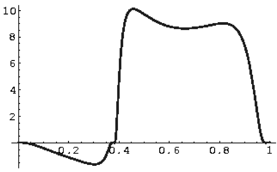
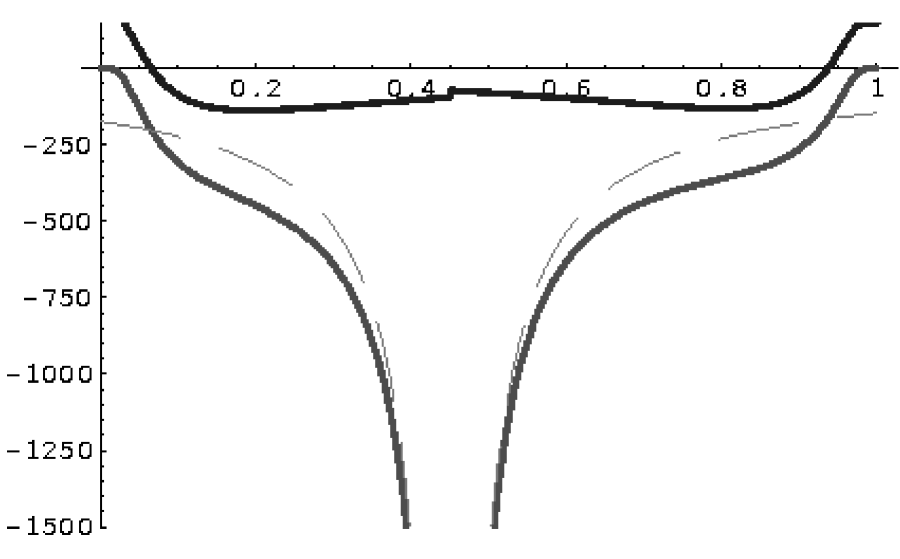
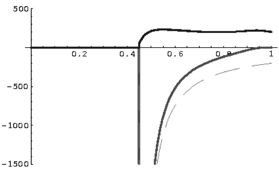
FIG. 16.: Examples of amplitudes S0, S1, S2 for some $x$ and $\zeta$ plotted as a function of $y$. Gray line is the original amplitude and dashed line is the IR-piece subtracted from it. IR piece is partially integrated analytically. The remaining amplitude (black) is integrated numerically in 5D using MC method.

In the reduced box-diagram (right in Fig.10), the struck parton momentum $k$ produces an UV-divergence because this amplitudes falls off like $1/{\bf k}_{\perp}^{2}$ as $|{\bf k}_{\perp}|\rightarrow\infty$. This results in a logarithmic UV-divergence. Note that, since the original box diagram is UV-finite, this UV-divergence is fictitious and is caused by the approximation for the effective vertex used herein, in which the struck parton momentum was neglected and its propagator was replaced with ${1/Q^{2}}$, a procedure that is admissible as long as $k^{2}\ll Q^{2}$. We may handle this singularity by using a cutoff $\Lambda^{2}$ of the order of $Q^{2}$. For $k^{2}\geq Q^{2}$, the struck parton propagator should behave as $1/{k^{2}}$. In principle, one may consider renormalization of this effective vertex to remove the dependence on $\Lambda$. However, we did not do this here because this term had only a weak dependence on the cutoff $\ln\Lambda^{2}\approx\ln Q^{2}$. In numerical calculations, we took this contribution in the form

$${\cal M}=\frac{(-\zeta)\,\overline{{\rm Tr}\,\,[\dots]}/Q^{2}}{\overline{{\rm Denominator}[\dots]}}\,h_{LF}h^{\prime}_{LF}(y,{\bf l}_{\perp})\times\frac{{\bf k}_{\perp}^{2}}{({\bf k}_{\perp}^{2}+m^{2})^{2}},$$ (B5)

and did the integration in ${\bf k}_{\perp}$ analytically:

$$B_{\Lambda}=\int\limits_{|{\bf k}_{\perp}|\leq\Lambda}d^{2}{\bf k}_{\perp}\,\frac{{\bf k}_{\perp}^{2}}{({\bf k}_{\perp}^{2}+m^{2})^{2}}=\pi\left\{\ln(1+\Lambda^{2}/m^{2})-\frac{\Lambda^{2}}{(m^{2}+\Lambda^{2})}\right\}.$$ (B6)

The remaining expression was integrated over $dyd^{2}{\bf l}_{\perp}$ and stored as “UV-contribution”. Finally, after these parts were subtracted, the residual part of the amplitude was integrated numerically in 5 dimensions using MC method.

For the convenience of using Monte-Carlo, the integration over $y$ was further reduced. Normally, the integration over $y$ would go over three regions, e.g. $y<x<\zeta$, $x<y<\zeta$ and $x<\zeta<y$ if $x<\zeta$. These three integrals were rescaled, e.g. $y=x\eta$ in $y<x<\zeta$, $y=x+(\zeta-x)\eta$ in $x<y<\zeta$ etc, so that $0<\eta<1$ and the three contributions, corresponding to these different regions, could be added together. Their sum, as a function of $\eta$, was the cumulative amplitude to be actually integrated with 5D Monte-Carlo (see Fig.17).

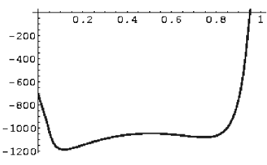
FIG. 17.: Example of cumulative amplitude as function of $\eta$ which was integrated with 5D Monte-Carlo.

The MC integration was organized in a series of bunches, each bunch containing $N_{i}\sim 100$ integrations using $M_{i}\sim 10,000$ points. Each bunch is treated as a “measurement” of the integral. When the test-points are independent in the MC-integration, each measurement (bunch) is independent from each other and the general principles of statistics can be applied. For each bunch, thus, we estimated the dispersion $\sigma_{i}$ and the mean $\mu_{i}$ of the measurement distribution. In this way, we estimated the value of the integral as well as the statistical error in each bunch from MC integrations. All bunches finally were combined with appropriate weight factors to produce the final estimate of the integral and MC-integration error. We tested our integration with different limits of integration in $({\bf k}_{\perp},{\bf l}_{\perp})$ to see if any accuracy is systematically lost due to finite bounds of integration in ${\bf k}_{\perp}$, ${\bf l}_{\perp}$. We observed that, except for rapid decrease of the MC-efficiency, no noticeable change occurred when the integration region was enlarged. Special attention was paid to $x=\zeta$ point since many of the amplitudes become singular in this case. Although all of these singularities are removable, we explicitly found the analytical limit in each expression for $x\rightarrow\zeta$ either from the left or from the right, and accommodated this in the final graphs as left (right) limit points at $x=\zeta$.

Thus, with our program we generated three different numbers for each point $x,\zeta$. These were “IR-contribution”, “UV-contribution” and the residual integrated amplitude. These were added to produce the final result

$${\cal M}_{\rm final}={\cal M}_{0}+f({\cal M}_{IR}+{\cal M}_{res}+B_{\Lambda}{\cal M}_{UV}),$$ (B7)

where ${\cal M}_{0}$ is the 0th-order amplitude, ${\cal M}_{IR}$ is IR-piece, ${\cal M}_{UV}$ is UV-piece of the amplitude and $B_{\Lambda}$ is the factor shown in Eq. (B6) with $\Lambda^{2}\approx Q^{2}$, where UV-cutoff $\Lambda\approx 5$ GeV was typically used. ${\cal M}_{res}$ is the MC-integrated remaining contribution. These results for $\zeta=0.3$ are plotted in Fig.18.

FIG. 18.: The plot of all contributions to scale for $\zeta=0.3$. The final result, “IR-contribution”, “UV-contribution” and the 5D residual integral are denoted by boxes, diamonds, stars and triangles, respectively.

One final note is in order. In the LFBS approach of Ref.[19], there is a free parameter $G_{\pi}$ which can be adjusted to fit the pion form factor as

$$\int^{1}_{0}{dx}\,{\cal F}_{\pi}(\zeta,x,t)=(1-\zeta/2)\,F_{\pi}(t)\,.$$ (B8)

In principle, $G_{\pi}$ may be allowed to depend on $t$ and $\zeta$. In that case one should solve for $G_{\pi}$ from Eq. (B8). To facilitate this process, we note that $G_{\pi}$ appears at most linearly from the non-valence final-state vertex in the final expressions. In our numerical procedure we explicitly separated $G_{\pi}^{0}$ and $G_{\pi}^{1}$ parts of the amplitudes and computed separately ${\cal M}^{0}_{f}$ and ${\cal M}^{1}_{f}$ so that

$${\cal M}_{f}={\cal M}^{0}_{f}+G_{\pi}{\cal M}^{1}_{f}.$$ (B9)

Then $G_{\pi}$ can be easily found from Eq. (B8) by solving a linear equation. In our calculations, however, we did not solve exactly for $G_{\pi}(t,\zeta)$, but used $G_{\pi}=0.32$ following the work of Ref.[20] where the justification can be found. Similar to Ref.[20], we find that the condition (B8) is satisfied well for all values of $\zeta$ even with a constant $G_{\pi}$.

REFERENCES

- [1] X. D. Ji, Phys. Rev. Lett. 78, 610 (1997), Phys. Rev. D 55, 7114 (1997).
- [2] A. V. Radyushkin, Phys. Lett. B 380, 417 (1996), Phys. Rev. D 56, 5524 (1997).
- [3] D. Muller, D. Robaschik, B. Geyer, F. M. Dittes and J. Horejsi, Fortsch. Phys. 42, 101 (1994).
- [4] X. D. Ji and J. Osborne, Phys. Rev. D 58, 094018 (1998).
- [5] J. C. Collins and A. Freund, Phys. Rev. D 59, 074009 (1999).
- [6] K. Goeke, M. V. Polyakov and M. Vanderhaeghen, Prog. Part. Nucl. Phys. 47, 401 (2001).
- [7] M. Diehl, Phys. Rept. 388, 41 (2003).
- [8] A. V. Belitsky and A. V. Radyushkin, Phys. Rept. 418, 1 (2005).
- [9] V. N. Gribov and L. N. Lipatov, Sov. J. Nucl. Phys. 15, 438 (1972).
- [10] G. Altarelli and G. Parisi, Nucl. Phys. B 126, 298 (1977).
- [11] Y. L. Dokshitzer, Sov. Phys. JETP 46, 641 (1977).
- [12] A. V. Efremov and A. V. Radyushkin, Theor. Math. Phys. 42, 97 (1980) Phys. Lett. B 94, 245 (1980).
- [13] G. P. Lepage and S. J. Brodsky, Phys. Lett. B 87, 359 (1979); Phys. Rev. D 22, 2157 (1980).
- [14] M. Diehl, T. Feldmann, R. Jakob and P. Kroll, Eur. Phys. J. C 8, 409 (1999).
- [15] M. Diehl, T. Feldmann, R. Jakob and P. Kroll, Nucl. Phys. B 596, 33 (2001) [Erratum-ibid. B 605, 647 (2001)].
- [16] S. J. Brodsky, M. Diehl and D. S. Hwang, Nucl. Phys. B 596, 99 (2001).
- [17] M. Burkardt, Phys. Rev. D 62, 071503 (2000) [Erratum-ibid. D 66, 119903 (2002)].
- [18] B. C. Tiburzi and G. A. Miller, Phys. Rev. D 65, 074009 (2002); B. C. Tiburzi and G. A. Miller, arXiv:hep-ph/0205109.
- [19] H.-M. Choi, C.-R. Ji and L. S. Kisslinger, Phys. Rev. D 64, 093006 (2001).
- [20] H.-M. Choi, C.-R. Ji and L. S. Kisslinger, Phys. Rev. D 66, 053011 (2002).
- [21] H.-M. Choi and C.-R. Ji, Phys. Rev. D 59, 074015 (1999).
- [22] H.-M. Choi and C.-R. Ji, Phys. Rev. D 56, 6010 (1997).
- [23] L. S. Kisslinger, H.-M. Choi and C.-R. Ji, Phys. Rev. D 63, 113005 (2001).
- [24] C.-R. Ji and H.-M. Choi, Phys. Lett. B 513, 330 (2001); eConf C010430: T23(2001) [hep-ph/0105248].
- [25] H.-M. Choi and C.-R. Ji, Phys. Lett. B 460, 461 (1999); Phys. Rev. D 59, 034001 (1999).
- [26] H.-M. Choi, C.-R. Ji and L. S. Kisslinger, Phys. Rev. D 65, 074032 (2002).
- [27] T. Frederico, J. H. O. Sales, B. V. Carlson and P. U. Sauer, Nucl. Phys. A 737, 260 (2004).
- [28] A. N. Kvinikhidze and B. Blankleider, Phys. Rev. D 68, 025021 (2003).
- [29] A. Airapetian et al. [HERMES Collaboration], Phys. Rev. Lett. 87, 182001 (2001).
- [30] S. Stepanyan et al. [CLAS Collaboration], Phys. Rev. Lett. 87, 182002 (2001).
- [31] B. C. Tiburzi and G. A. Miller, Phys. Rev. D 67, 054014 (2003).
- [32] B. C. Tiburzi and G. A. Miller, Phys. Rev. D 67, 054015 (2003).
- [33] X. D. Ji, W. Melnitchouk and X. Song, Phys. Rev. D 56, 5511 (1997).
- [34] A. V. Radyushkin, Phys. Lett. B 449, 81 (1999).
- [35] A. V. Radyushkin, Phys. Rev. D 59, 014030 (1999).
- [36] B. C. Tiburzi and G. A. Miller, Phys. Rev. D 67, 013010 (2003).
- [37] N. Kivel, . V. Polyakov and M. Vanderhaeghen, Phys. Rev. D 63, 114014 (2001).
- [38] A. Freund and M. McDermott, Eur. Phys. J. C 23, 651 (2002).
- [39] S. J. Brodsky, C.-R. Ji and M. Sawicki, Phys. Rev. D 32, 1530 (1985).
- [40] J. H. O. Sales, T. Frederico, B. V. Carlson and P. U. Sauer, Phys. Rev. C 61, 044003 (2000).
- [41] A. Mukherjee, I. V. Musatov, H. C. Pauli and A. V. Radyushkin, Phys. Rev. D 67, 073014 (2003).
- [42] B. C. Tiburzi, W. Detmold and G. A. Miller, Phys. Rev. D 68, 073002 (2003).