A D-brane inspired Trinification model.

We describe the basic features of model building in the context of intersecting D-branes. As an example, a D-brane inspired construction with $U(3)_{C}\times U(3)_{L}\times U(3)_{R}$ gauge symmetry is proposed -which is the analogue of the Trinification model- where the unification porperties and some low energy implications on the fermion masses are analysed.

 

^∗Talk presented at the “Corfu Summer Institute”, Corfu-Greece, September 4-14, 2005

1. Introduction

Model building establishes the connection between the mathematical formulation of a physics theory and the known (experimentally discovered) world of elementary particles. In High Energy Physics the “known world” is defined as the one which is described by the Standard Model (SM). The SM spectrum, consists of three flavors of LH lepton doublets and quarks, the RH electrons, up and down quarks respectively plus gauge bosons and the Higgs field (although not yet discovered).

During the last three decades we have learned a lot from the attempts to extend the SM. As early as 1974, the observation that gauge couplings converge at large scales, suggested unification of the three forces at a scale $M_{U}\sim 10^{15}$ GeV. This observation led to the incorporation of the SM into a gauge group with higher symmetry i.e., $SU(5)$ etc (Grand Unification). A number of Grand Unified Theories (GUTs) (Pati-Salam model, SO(10) GUT etc ) predicted also the existence of the RH neutrino. Its existence can lead to a light Majorana mass (through the see-saw mechanism) which is now confirmed by the present experimental data. Next, the incorporation of supersymmetry [2] into the game of unification had a big success: This was the solution of the hierarchy, which was a fatal problem in all non-supersymmetric GUTs. However, the cost to pay was the doubling of the spectrum, with the inclusion of superpartners and many arbitrary parameters. For example, the number of arbitrary parameters one counts in the Minimal Supersymmetric Standard Model (MSSM) are pretty much above 100. String theory model building went a bit further: For instance, one could calculate from the first principles of the theory the Yukawa couplings [3]. Non-renormalizable contributions of the form $\epsilon^{n}Qu^{c}h$, $\epsilon=\frac{\langle\phi\rangle}{M_{S}}$, (and similar terms for the other masses), where $\phi$ is a singlet and $M_{S}$ the string scale, were also calculated to any order. This gave the possibility to determine the structure of the fermion mass matrices in terms of a few known expansion parameters[4].

This kind of mass textures gives rise to successful hierarchies of the form $m_{u}:m_{c}:m_{t}$ $\sim\epsilon^{6}:\epsilon^{2}:1$ up to order one coefficients (and similarly for the other fermions). A number of other phenomenological problems however, were not resolved even in the string context. For example, there was no systematic way of eliminating baryon violating operators of any dimension, since, even if they are absent at the three level (due to the existence of a possible symmetry), they generally appear in higher order corrections. Another aesthetically and experimentally unpleasant fact is that the string scale which, in all models obtained from the heterotic string theory, is of the order of the Planck scale [5]. Yet, the non-discovery of the superpartners at energies expected to be there, is also another headache.

It now appears that many of the above unanswered questions and puzzles might have a solution in models built in the context of branes immersed in higher dimensions [6]. Indeed, the models built in this context offer possibilities for solving the above problems: a class of them allows a low unification scale of the order of a few TeV [7], therefore supersymmetry is not necessary since there is no hierarchy problem; further, in certain cases, (type I string theory) the presence of internal magnetic fields[8] provides a concrete realization of split supersymmetry [9], therefore, intermediate or higher string scales are also possible in this case[10]. Further, the gauge group structure obtained in these models contains $U(1)$ global symmetries, one of them associated with the baryon number, so that baryon number violation is prohibited to all orders in perturbation theory.

2. Intersecting branes

In the construction of D-brane models the basic ingredient is the brane stack, i.e. a certain number of parallel, almost coincident D-branes. A single D-brane carries a $U(1)$ gauge symmetry which is the result of the reduction of the ten-dimensional Yang-Mills theory. A stack of $N$ parallel branes gives rise to a $U(N)$ gauge theory where the gauge bosons correspond to open strings having both their ends attached to some of the branes of the various stacks. The compact space is taken to be a six-dimensional torus $T^{6}=T^{2}\times T^{2}\times T^{2}$, however, for simplicity, let us assume first the intersections on a single $T^{2}$. $D$-branes in flat space lead to non-chiral matter. Chirality arises when they are wrapped on a torus. In this case chiral fermions sit in singular points in a transverse space while the number of fermion generations [11, 12], and other fermions in intersecting branes are related to the two distinct numbers of wrappings of the branes around the two circles $R_{1},R_{2}$ of the torus . Consider intersecting D6-branes filling the four-dimensional space-time with $(n,m)$ wrapping numbers. (This means that we wrap $n$-times the brane along the circle of $R_{1}$ radius and $m$-times along $R_{2}$.) For two stacks $N_{a},N_{b}$, we denote with $(n_{a},m_{a})$ and $(n_{b},m_{b})$ the wrappings respectively. The gauge group is $U(N_{a})\times U(N_{b})$ while the fermions (which live in the intersections) belong to the bi-fundamental $(N_{a},\bar{N}_{b})$, (or $(\bar{N}_{a},N_{b})$). We may also obtain representations in $(N_{a},N_{b^{*}})$ from strings attached on the branes $a,b^{*}$, where $b^{*}$ is the mirror of the $b$-brane under the $\Omega\,R$ operation, $\Omega$ beeing the whorld-sheet parity operation and $R$ a geometrical action. The number of the intersections on the two-torus is given by $I_{ab}=n_{a}m_{b}-m_{a}n_{b}$, for $(N,\bar{N})$ and $I_{ab^{*}}=n_{a}m_{b}+m_{a}n_{b}$ for $(N_{a},N_{b^{*}})$. These also equal the number of the chiral fermion representations obtained at the intersections. Additional pairs can be constructed by the action on the vector $\vec{v}=(n,m)$ with the $SL(2,Z)$. The latter preserves the intersection numbers, therefore it preserves also the number of chiral fermions. The $SL(2,Z)$ elements act:

$$\left(\begin{array}[]{c}n^{\prime}\\ m^{\prime}\\ \end{array}\right) = \left(\begin{array}[]{cc}a&b\\ c&d\\ \end{array}\right)\,\left(\begin{array}[]{c}n\\ m\\ \end{array}\right)$$ (7)

(Since $ad-bc=1$, it follows $n_{a}^{\prime}m_{b}^{\prime}-m_{a}^{\prime}n_{b}^{\prime}=n_{a}m_{b}-m_{a}n_{b}$.)

The gauge couplings of the theory are given as follows: Let $g$ be the metric on the torus

$$g = (2\pi)^{2}\left(\begin{array}[]{cc}R_{1}^{2}&R_{1}R_{2}\cos\theta\\ R_{1}R_{2}\cos\theta&R_{2}^{2}\\ \end{array}\right)$$ (10)

where $\theta$ is the angle of the two vectors defining the torus lattice. The length of the $\vec{v}=(n,m)$ wrapping, is then $\ell_{nm}=\sqrt{g_{ab}v^{a}v^{b}}$, i.e.,

$$\ell_{mn} = 2\pi\sqrt{n^{2}R_{1}^{2}+m^{2}R_{2}^{2}+2nmR_{1}R_{2}\cos\theta}$$ (11)

The gauge coupling $g_{a}$ of the $a^{th}$ group is given by

$$\frac{4\pi^{2}}{g_{a}^{2}} = \frac{M_{S}}{\lambda_{II}}\ell_{m_{a}n_{a}}$$ (12)

where $M_{S}$ is the string scale, $\lambda_{II}$ is the type-II string coupling and $\ell_{m_{a}n_{a}}$ is given by (11). Yukawa coefficients are also calculable in these constructions in terms of geometric quantities (area) of the torus[11, 12]. For example, the size of the Yukawa coupling $y_{ijk}$ for a square torus is

$$y_{ijk} = e^{-\frac{R_{1}R_{2}}{\alpha^{\prime}}A_{ijk}}$$ (13)

where $A_{ijk}$ is the area of the world-sheet connecting three vertices, scaled by the area of the torus.

We may generalize these results, considering compactifications on a 6-torus factorized as $T^{6}=T^{2}\times T^{2}\times T^{2}$. For example, if we denote $(n_{a}^{i},m_{a}^{i})$ the wrapping numbers of the D6_a brane around the $i^{th}$ torus, the number of intersections is given by the product of the intersections in each of them

$$I_{ab} = \prod_{i=1}^{3}(n_{a}^{i}m_{b}^{i}-n_{b}^{i}m_{a}^{i}),\;\;{\rm for}\;(N_{a},\bar{N}_{b})$$ (14)

$$I_{ab^{*}} = \prod_{i=1}^{3}(n_{a}^{i}m_{b}^{i}+n_{b}^{i}m_{a}^{i}),\;\;{\rm for}\;(N_{a},N_{b}^{*})$$ (15)

while cancellation of the $U(N)$ anomalies requires that the spectrum should satisfy $\sum_{b}\,I_{ab}N_{b}=0$. To satisfy this critirion, one usualy has to add additional matter states. For example, the fulfilment of this requirement in deriving the Standard Model in [13] led to the introduction of the right-handed neutrinos. We should note that further consistency conditions, as the cancellation of RR-tadpoles for theories [11] with open string sectors should be satisfied by $n_{a}^{i},m_{a}^{i}$.

Due to the fact that D-brane constructions generate $U(N)$ symmetries, from $U(N)_{a}\rightarrow SU(N)_{a}\times U(1)_{a}$, we conclude that several $U(1)$ factors appear in these models. For, example, the derivation of the SM may be obtained from a set of $U(3),U(2)$ and several $U(1)$ brane stacks, leading to a symmetry[14, 15]

$${U(3)}_{C}\times{U(2)}_{L}\times\prod_{i=1}^{n}{U(1)}^{i}={SU(3)}_{C}\times{SU(2)}_{L}\times U(1)_{C}\times U(1)_{L}\times\prod_{i=1}^{n}{U(1)}^{i}$$ (16)

Fermion and Higgs representations are charged under $U(1)_{C,L,i}$. Some of these $U(1)$ symmetries, play a particular role in the low energy effective theory. For example, $U(1)_{C}$ is related to baryon number, since all quarks carry the same $U(1)_{C}$-charge. Thus, all global symmetries of SM are gauge symmetries in the context of D-brane constructions. Further, the $U(1)$ factors have mixed anomalies with the non-abelian groups $SU(N_{a})$ given by $A_{ab}=(I_{ab}-I_{a^{*}b})N_{a}/2$. It happens that one linear combination remains anomaly free and contributes to the hypercharge generator which in general is a linear combination of the form

$$Q_{Y} = \sum_{m}^{n+2}c_{m}\,Q_{m}$$ (17)

where the $c_{m}$ are to be specified in terms of the hypercharge assignment of the particle spectrum of a given D-brane construction. The remaining $U(1)$ combinations carry anomalies which are cancelled by a generalized Green-Schwartz mechanism and the corresponding gauge bosons become massive. These symmetries however, persist in the low-energy theory as global symmetries.

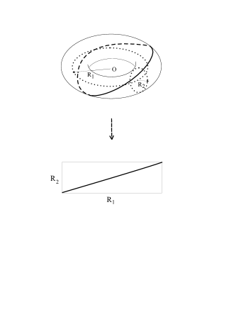
Figure 1: Schematic representation of a $(1,1)$ D-brane wrapping on a $T^{2}$ torus.

3. A $U(3)^{3}$ brane inspired model

We now present a specific non-supersymmetric example with gauge symmetry $U(3)^{3}$ which can be considered as the analogue of the “Trinification” model proposed long time ago [17, 18] . We will therefore describe here the steps one has to follow for a viable D-brane construction. To generate this group one needs three stacks of D-branes, each stack containing 3 parallel almost coincident branes in order to form the $U(3)$ symmetry. We write the complete gauge symmetry as

$$U(3)_{C}\times U(3)_{L}\times U(3)_{R},$$

so that the first $U(3)$ is related to $SU(3)$ color, the second involves the weak $SU(2)_{L}$ and the third is related to a possible intermediate $SU(2)_{R}$ gauge group. Since $U(3)\rightarrow SU(3)\times U(1)$, we conclude that, in addition to the $SU(3)^{3}$ gauge group, the D-brane construction contains also three extra $U(1)$ abelian symmetries. The $U(1)$ symmetry obtained from the color $U(3)_{C}\rightarrow SU(3)_{C}\times U(1)_{C}$ is related to the baryon number [14]. All baryons have the same charge under $U(1)_{C}$ and consequently this $U(1)$ is identified with a gauged baryon number symmetry. There are two more abelian factors from the chains $U(3)_{L}\rightarrow SU(3)_{L}\times U(1)_{L}$, $U(3)_{R}\rightarrow SU(3)_{R}\times U(1)_{R}$ so the final symmetry can be written

$$SU(3)_{c}\times SU(3)_{L}\times SU(3)_{R}\times U(1)_{C}\times U(1)_{L}\times U(1)_{R}$$ (18)

The abelian $U(1)_{C,L,R}$ factors have mixed anomalies with the non-abelian $SU(3)^{3}$ gauge part with are determined by the contributions of three fermion generations. There is an anomaly free combination, namely [27]

$$U(1)_{{\cal Z}^{\prime}} = U(1)_{C}+U(1)_{L}+U(1)_{R}$$ (19)

which contributes to the hypercharge, while the two remaining combinations are anomalous; these anomalies are cancelled by a generalized Green-Schwarz mechanism.

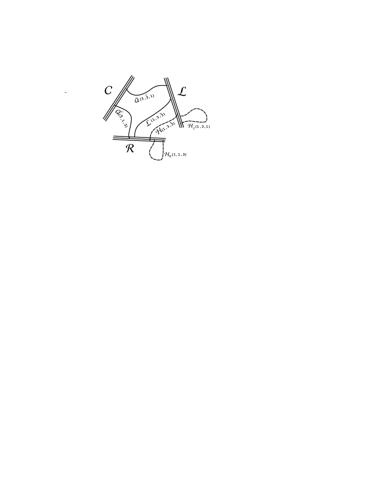
Figure 2: Schematic representation of a $U(3)_{C}\times U(3)_{L}\times U(3)_{R}$ D-brane configuration and the matter fields of the model.

The possible representations which arise in this scenario should accommodate the standard model particles and the necessary Higgs fields to break the $U(3)^{3}$ symmetry down to SM. The spectrum of a D-brane model involves two kinds of representations, those obtained when the two string ends are attached to two different branes and those whose both ends are on the same brane stack. In figure 3 we show the minimum number of irreps required to accommodate the fermions and appropriate Higgs fields. Under (18) these states obtained from strings attached to two different branes have the following quantum numbers

$${\cal Q^{\hphantom{c}}} = (3,\bar{3},1)_{(+1,-1,\hphantom{+}0)}$$ (20)

$${\cal Q}^{c} = (\bar{3},1,3)_{(-1,\hphantom{+}0,+1)}$$ (21)

$${\cal L}^{\hphantom{c}} = (1,3,\bar{3})_{(\hphantom{+}0,+1,-1)}$$ (22)

$${\cal H}^{\hphantom{c}} = (1,3,\bar{3})_{(\hphantom{+}0,+1,-1)}$$ (23)

while the states arising from strings with both ends on the same 3-stack are

$${\cal H}_{\cal L} = (1,3,1)_{(0,-2,0)}$$ (24)

$${\cal H}_{\cal R} = (1,1,3)_{(0,0,-2)}$$ (25)

Under $SU(3)_{L}\times SU(3)_{R}$ $\rightarrow$ $\left[SU(2)_{L}\times U(1)_{L^{\prime}}\right]\,\times\,\left[U(1)_{R^{\prime}}\times U(1)_{\Omega}\right]$ and the $U(1)_{{\cal Z}^{\prime}}$, we employ the hypercharge embedding

$$Y=-\frac{1}{6}X_{L^{\prime}}+\frac{1}{3}X_{R^{\prime}}+\frac{1}{6}{\cal Z}^{\prime}$$ (26)

where $X_{L^{\prime}},X_{R^{\prime}},{\cal Z}^{\prime}$ represent the generators of the corresponding $U(1)$ factors. Under the symmetry $SU(3)_{C}\times SU(2)_{L}\times U(1)_{Y}\times U(1)_{\Omega}$ (20-25) decompose as follows

$${\cal Q}^{\hphantom{c}} = q\left(3,2;\frac{1}{6},0_{\Omega}\right)+g\left(3,1;-\frac{1}{3},0_{\Omega}\right)$$ (27)

$${\cal Q}^{c} = d^{c}\left(\bar{3},1;\frac{1}{3},1_{\Omega}\right)+u^{c}\left(\bar{3},1;-\frac{2}{3},0_{\Omega}\right)+g^{c}\left(\bar{3},1;\frac{1}{3},-1_{\Omega}\right)$$ (28)

$${\cal L}^{\hphantom{c}} = \ell^{+}\left(1,2;-\frac{1}{2},1_{\Omega}\right)+\ell^{-}\left(1,2;-\frac{1}{2},-1_{\Omega}\right)+{\ell^{c}}\left(1,2;+\frac{1}{2},0_{\Omega}\right)$$ (29)

$$+\nu^{c+}(1,1;0,1_{\Omega})+\nu^{c-}(1,1;0,-1_{\Omega})+e^{c}(1,1;1,0_{\Omega})$$

$${\cal H} = (1,3,\bar{3})=h^{d+}\left(1,2;-\frac{1}{2},1\right)+h^{d-}\left(1,2,-\frac{1}{2},-1\right)+{h^{u}}\left(1,2;\frac{1}{2},0\right)$$ (30)

$$+{e_{H}^{c}}(1,1;1,0)+{\nu_{H}^{c+}}(1,1;0,1)+{\nu_{H}^{c-}}(1,1;0,-1),\;\;\;$$

$${\cal H}_{\cal L} = (1,3,1)=\hat{h}_{L}^{+}\left(1,2;-\frac{1}{2},0\right)+\hat{\nu}_{{\cal H}_{\cal L}}\left(1,1;1,0\right)$$ (31)

$${\cal H}_{\cal R} = (1,1,3)={\hat{e}_{H}^{c}}(1,1;1,0)+{\hat{\nu}_{{\cal H}_{\cal R}}^{c+}}(1,1;0,1)+\hat{\nu}_{{\cal H}_{\cal R}}^{c-}(1,1;0,-1)$$ (32)

Representation (27) includes the left handed quark doublets and an additional colored triplet with quantum numbers as those of the down quark, while representation (28) contains the right-handed partners of (27). Further, (29) involves the lepton doublet, the right-handed electron and its corresponding neutrino, two additional $SU(2)_{L}$ doublets and another neutral state, called neutreto[17]. The Higgs sector consists of (30) which is the same representation as that of the lepton fields, and the left and right triplets (31) and (32) respectively.

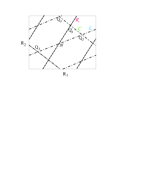
Figure 3: Schematic representation of the intersections on a $T^{2}$ for a three-generation $U(3)_{C}\times U(3)_{L}\times U(3)_{R}$ D-brane model.

3.1 Mass scales, Symmetry breaking and Yukawa couplings

3.1.1 Mass scales

The reduction of the ${SU(3)}^{3}\times{U(1)}^{3}$ to the SM is in general associated with three different scales corresponding to the $SU(3)_{R}$, $SU(3)_{L}$ and $U(1)_{{\cal Z}^{\prime}}$ symmetry breaking. We will assume here for simplicity that the $SU(3)_{L,R}$ and $U(1)_{{\cal Z}^{\prime}}$ symmetries break simultaneously at a common scale $M_{R}$, hence the model is characterized only by two large scales, the String/brane scale $M_{S}$, and the scale $M_{R}$. Clearly, the $M_{R}$ scale cannot be higher than $M_{S}$, i.e., $M_{R}\leq M_{S}$, and the equality holds if the $SU(3)_{R}\times SU(3)_{L}$ symmetry breaks directly at $M_{S}$. In a D-brane realization of the proposed model, since the three $U(3)$ gauge factors originate from 3-brane stacks that span different directions of the higher dimensional space, the corresponding gauge couplings $\alpha_{C,L,R}$ are not necessarily equal at the string scale $M_{S}$. However, in certain constructions, at least two D-brane stacks can be superposed and the associated couplings are equal[14]. In our bottom up approach, a crucial role in the determination of the scales $M_{R,S}$ is played by the neutrino physics. More precisely, in order to obtain the correct scale for the light neutrino masses, which are obtained through a see-saw mechanism and are found to be of the order $m_{\nu}\sim m_{W}^{2}/M_{S}$, the string scale $M_{S}$ should be in the range $M_{S}\sim 10^{13}-10^{15}$ GeV. In order to determine the range of $M_{S},M_{R}$, we use as inputs the low energy data for $\alpha_{3},\alpha_{em}$ and $\sin^{2}\theta_{W}$ and perform a one-loop renormalization group analysis. The cases $\alpha_{L}=\alpha_{R}$ and $\alpha_{R}=\alpha_{C}$ presented in Table 1 are found to be consistent with the neutrino data.

model	$M_{R}/GeV$	${M_{S}}/{GeV}$
$a_{L}=a_{R}$	$1.7\times 10^{9}$	$>1.7\times 10^{9}$
$a_{L}=a_{C}$	$<2.3\times 10^{16}$	$>2.3\times 10^{16}$
$a_{C}=a_{R}$	$<2.3\times 10^{11}$	$>2.3\times 10^{11}$

Table 1: Upper and lower bounds for $SU(3)_{R}$ breaking scale ($M_{R}$) and the corresponding String scale ($M_{S}$) for the three cases $a_{L}=a_{C}$, $a_{R}=a_{C}$ and $a_{L}=a_{R}$.

In particular, we find that the case $\alpha_{L}=\alpha_{R}$ predicts $M_{R}$ constant, i.e., independent of the common gauge coupling $a\equiv\alpha_{L}=\alpha_{R}$ and $M_{S}$ also in the required region. For $\alpha_{R}=\alpha_{C}$, we also obtain $M_{S}\geq 2.3\times 10^{11}$GeV.

3.1.2 The Symmetry breaking

The Higgs states (30-32) are sufficient to break the original gauge symmetry $U(3)^{3}$ down to the Standard Model[27], however, according to ref[17], a non-trivial KM mixing and quark mass relations would require at least two Higgs fields in $(1,3,\bar{3})$. We should mention however, that in string or intersecting brane models, Yukawas are calculable in terms of geometric quantities -such as torus area- thus, from this point of view a second Higgs is not necessary. To break the symmetry and provide with masses the various matter multiplets we assume two Higgs in $(1,3,\bar{3})$ and a pair ${\cal H}_{\cal L}=(1,3,1)$, ${\cal H}_{\cal R}=(1,1,3)$ with the following vevs:

$${\cal H}_{1} \rightarrow \langle h^{u}_{1}\rangle=u_{1},\;\langle h^{d-}_{1}\rangle=u_{2},\;\langle{{\nu^{c+}_{H,}}_{1}}\rangle=U,$$

$${\cal H}_{2} \rightarrow \langle h^{u}_{2}\rangle=v_{1},\;\langle{h^{d-}}_{2}\rangle=v_{2},\;\langle{h^{d+}}_{2}\rangle=v_{3},\langle{\nu^{c-}_{H}}_{2}\rangle=V_{1},\;\langle{\nu^{c+}_{H}}_{2}\rangle=V_{2}$$

$${\cal H}_{\cal L} \rightarrow \langle\hat{\nu}_{H_{L}}\rangle=A_{L}$$

$${\cal H}_{\cal R} \rightarrow \langle\hat{\nu}_{H_{R}}\rangle=A_{R}$$

The vevs $U,V_{1,2}$ and $A_{L,R}$ are taken of the order $M_{R}$, while $u_{1,2}$ and $v_{1,2}$ are of the order of the electroweak scale.

3.1.3 Fermion masses

In the present $U(3)^{3}$ construction, due to the existence of the additional $U(1)_{C,L,R}$ symmetries, the following Yukawa coupling is present at the tree-level Yukawa potential

$$\lambda_{Q,1}^{ij}{\cal Q}_{i}\,{\cal Q}_{j}^{c}\,{\cal H}_{a},\;\;{a=1,2}$$ (33)

It can provide quark masses as well masses for the extra triplets. For the up quarks

$$m_{uu^{c}}^{ij} = \lambda_{Q,1}^{ij}u_{1}+\lambda_{Q,2}^{ij}v_{1}$$ (34)

For the down-type quarks $d_{i},d_{j}^{c},g_{i},g_{j}^{c}$, we obtain a $6\times 6$ down type quark matrix in flavour space, of the form

$$m_{d} = \left(\begin{array}[]{cc}m_{dd^{c}}&M_{gd^{c}}\\ m_{dg^{c}}&M_{gg^{c}}\end{array}\right)$$ (37)

where $m_{dd^{c}}=\lambda_{Q,1}^{ij}\,u_{2}+\lambda_{Q,2}^{ij}\,v_{2}$ and $m_{dg^{c}}=\lambda_{Q,2}^{ij}\,v_{3}$ are $3\times 3$ matrices with entries of the electroweak scale, while $M_{gd^{c}}=\lambda_{Q,2}^{ij}\,V_{1}$, $M_{gg^{c}}=\lambda_{Q,1}^{ij}\,U+\lambda_{Q,2}^{ij}\,V_{2}$ are of the order $M_{R}$. The diagonalization of the non-symmetric mass matrix (37) will lead to a light $3\times 3$ mass matrix for the down quarks and a heavy analogue of the order of the $SU(3)_{R}$ breaking scale.

The extra $U(1)_{C,L,R}$ factors do not allow for a tree-level coupling for the lepton fields. The lowest order allowed leptonic Yukawa terms arise at fourth order. These are

$$\frac{f_{ij}^{ab}}{M_{S}}\,{\cal H}_{a}^{\dagger}\,{\cal H}_{b}^{\dagger}\,{\cal L}_{i}\,{\cal L}_{j}+\frac{\zeta_{ij}}{M_{S}}\,{\cal H}_{\cal L}\,{\cal H}_{\cal R}^{\dagger}\,{\cal L}_{i}\,{\cal L}_{j}$$ (38)

where $f_{ij}^{ab},\zeta_{ij}$ are order one Yukawa couplings, and $a,b=1,2$. These terms provide with masses the charged leptons suppressed by a factor $M_{R}/M_{S}$ compared to quark masses. Thus, a natural quark-lepton hierarchy arises in this model. They further imply light Majorana masses for the three neutrino species through a see saw mechanism. All the remaining states (lepton like doublets and neutral singlets) obtain masses of the order $M_{R}^{2}/M_{S}$[27].

4. Conclusions

In this talk, we have described the basic features of model building in the context of intersecting D-branes. As an example, we have analysed a D-brane analogue of the trinification model which can be generated by three separate stacks of D-branes. Each of the three stacks is formed by three identical branes, resulting to an $U(3)_{C}\times U(3)_{L}\times U(3)_{R}$ gauge symmetry for the model. Since $U(3)\rightarrow SU(3)\times U(1)$, this symmetry is equivalent to the standard $SU(3)^{3}$ trinification gauge group supplemented by three abelian factors $U(1)_{C,L,R}$. The main characteristics of the model are:

$\bullet$ The three $U(1)$ factors define an unique anomaly-free combination $U(1)_{{\cal Z}^{\prime}}=U(1)_{C}+U(1)_{L}+U(1)_{R}$ as well as two other anomalous combinations whose anomalies can be cancelled by a generalized Green-Schwarz mechanism.

$\bullet$ The Standard Model fermions are represented by strings attached to two different brane-stacks and belong to $(3,\bar{3},1)+(\bar{3},1,3)+(1,3,\bar{3})$ representations as is the case of the trinification model.

$\bullet$ The scalar sector contains Higgs fields in $(1,3,\bar{3})$ (which is the same representation which accommodates the lepton fields), as well as Higgs in (1,3,1) and (1,1,3) representations which can arise from strings whose both ends are attached on the same brane stack. The Higgs fields break the $SU(3)_{L}\times SU(3)_{R}$ part of the gauge symmetry down to $U(1)_{em}$; they further provide a natural quark-lepton hierarchy since quark masses are obtained from tree-level couplings, while, due to the extra $U(1)$ symmetries, charged leptons are allowed to receive masses from fourth order Yukawa terms.

$\bullet$ The $SU(3)_{R}$ breaking scale is found to be $M_{R}>10^{9}$ GeV, while a string scale $M_{S}\sim 10^{13-15}$GeV is predicted which suppresses the light Majorana masses through a see-saw mechanism down to sub-eV range as required by neutrino physics.

Ackmowledgements. This research was co-funded by the European Union in the framework of the program ”Pythagoras I” (no. 1705 project 23) of the ”Operational Program for Education and Initial Vocational Training” of the 3rd Community Support Framework of the Hellenic Ministry of Education, funded by 25% from national sources and by 75% from the European Social Fund (ESF).

References

- [1] P. Langacker, “Grand Unified Theories And Proton Decay,” Phys. Rept. 72 (1981) 185.
-
[2]
H. P. Nilles,
Phys. Rept. 110 (1984) 1.
A. B. Lahanas and D. V. Nanopoulos, Phys. Rept. 145, 1 (1987). -
[3]
G. K. Leontaris and J. Rizos,
Nucl. Phys. B 554 (1999) 3
[arXiv:hep-th/9901098],
I. Antoniadis, G. K. Leontaris and J. Rizos, Phys. Lett. B 245 (1990) 161.
A. E. Faraggi, Phys. Lett. B 274 (1992) 47. - [4] L. E. Ibanez and G. G. Ross, “Fermion masses and mixing angles from gauge symmetries,” Phys. Lett. B 332 (1994) 100 [arXiv:hep-ph/9403338].
-
[5]
V. S. Kaplunovsky,
Nucl. Phys. B 307 (1988) 145
[Erratum-ibid. B 382 (1992) 436]
[arXiv:hep-th/9205068].
P. H. Ginsparg, Phys. Lett. B 197 (1987) 139.
K. R. Dienes, Phys. Rept. 287 (1997) 447 [arXiv:hep-th/9602045]. - [6] J. Polchinski, “Lectures on D-branes,” arXiv:hep-th/9611050.
-
[7]
C. P. Bachas,
JHEP 9811 (1998) 023
[arXiv:hep-ph/9807415].
N. Arkani-Hamed, S. Dimopoulos and G. R. Dvali, Phys. Lett. B 429 (1998) 263 [arXiv:hep-ph/9803315].
I. Antoniadis and B. Pioline, Nucl. Phys. B 550 (1999) 41 [arXiv:hep-th/9902055]. - [8] C. Bachas, hep-th/9503030.
- [9] I. Antoniadis and S. Dimopoulos, Nucl. Phys. B 715 (2005) 120 [arXiv:hep-th/0411032].
-
[10]
N. Arkani-Hamet and S. Dimopoulos,
hep-th/0405159;
G.F. Giudice and A. Romaninio, hep-ph/0406088. -
[11]
R. Blumenhagen, L. Goerlich, B. Kors and D. Lust, “Noncommutative
compactifications of type I strings on tori with magnetic
background flux,” JHEP 0010 (2000) 006 [hep-th/0007024].
R. Blumenhagen, B. Kors, D. Lust and T. Ott, “The standard model from stable intersecting brane world orbifolds,” Nucl. Phys. B 616 (2001) 3 [arXiv:hep-th/0107138]. -
[12]
G. Aldazabal, S. Franco, L. E. Ibanez, R. Rabadan and
A. M. Uranga, “Intersecting brane worlds,” JHEP 0102
(2001) 047 [hep-ph/0011132].
D. Cremades, L. E. Ibanez and F. Marchesano, JHEP 0307 (2003) 038 [arXiv:hep-th/0302105].
H. Verlinde and M. Wijnholt, arXiv:hep-th/0508089. - [13] L. E. Ibanez, F. Marchesano and R. Rabadan, JHEP 0111 (2001) 002 [arXiv:hep-th/0105155].
-
[14]
I. Antoniadis, E. Kiritsis and T. N. Tomaras, “A D-brane
alternative to unification,” Phys. Lett. B 486 (2000) 186
[hep-ph/0004214].
I. Antoniadis, E. Kiritsis, J. Rizos and T. N. Tomaras, Nucl. Phys. B 660 (2003) 81 [arXiv:hep-th/0210263].
C. Coriano, N. Irges and E. Kiritsis, arXiv:hep-ph/0510332. - [15] D. V. Gioutsos, G. K. Leontaris and J. Rizos, Eur. Phys. J. C 45 (2006) 241 [arXiv:hep-ph/0508120].
- [16] A.M. Uraga, Class. Quantum Grav.22(2005)S41-S76.
- [17] S. L. Glashow, “Trinification Of All Elementary Particle Forces,” Print-84-0577 (BOSTON).
- [18] A. Rizov, “A Gauge Model Of The Electroweak And Strong Interactions Based On The Group ,” Bulg. J. Phys. 8 (1981) 461.
- [19] K. S. Babu, X. He and S. Pakvasa, “Neutrino Masses And Proton Decay Modes In Trinification,” Phys. Rev. D 33 (1986) 763.
- [20] K. S. Babu, X. He and S. Pakvasa, Trinification,” Phys. Rev. D 33 (1986) 763.
- [21] G. R. Dvali and Q. Shafi, Phys. Lett. B 339 (1994) 241 [arXiv:hep-ph/9404334].
- [22] G. Lazarides and Q. Shafi, Nucl. Phys. B 329 (1990) 182.
- [23] N. Maekawa and Q. Shafi, Prog. Theor. Phys. 109 (2003) 279 [arXiv:hep-ph/0204030].
- [24] F. Gürsey and M. Serdanoglu, Lett. Nuovo Cimento, 21 (1978)28.
- [25] B. R. Greene, K. H. Kirklin, P. J. Miron and G. G. Ross, Nucl. Phys. B 278 (1986) 667.
-
[26]
K. S. Choi and J. E. Kim,
Phys. Lett. B 567 (2003) 87
[arXiv:hep-ph/0305002].
S. Willenbrock, Phys. Lett. B 561 (2003) 130 [arXiv:hep-ph/0302168].
C. D. Carone and J. M. Conroy, Phys. Rev. D 70 (2004) 075013 [arXiv:hep-ph/0407116].
J. Sayre, S. Wiesenfeldt and S. Willenbrock, arXiv:hep-ph/0601040. - [27] G. K. Leontaris and J. Rizos, Phys. Lett. B 632 (2006) 710 [arXiv:hep-ph/0510230].