Abstract

The origin of the most energetic cosmic ray events, with $E\raisebox{-3.69899pt}{~{}\shortstack{$>$ \\ [-0.07cm] $\sim$}}~{}10^{20}$ eV, remains mysterious. One possibility is that they are produced in the decay of very massive, long–lived particles. It has been suggested that these so–called “top–down scenarios” can be tested by searching for ultrarelativistic neutralinos, which would be produced copiously if superparticles exist at or near the TeV scale. In this paper we present a detailed analysis of the interactions of such neutralinos with ordinary matter. To this end we compute several new contributions to the total interaction cross section; in particular, the case of higgsino–like neutralinos is treated for the first time. We also carefully solve the transport equations. We show that a semi–analytical solution that has been used in the literature to treat the somewhat analogous propagation of $\tau$ neutrinos leads to large errors; we therefore use a straightforward numerical method to solve these integro–differential equations.

1 Introduction

Experiments like Fly’s Eye [1] and AGASA [2] have shown the existence of cosmic rays with energy $E\raisebox{-3.69899pt}{~{}\shortstack{$>$ \\ [-0.07cm] $\sim$}}~{}10^{20}$ eV, the so–called ultra high energy (UHE) component of the cosmic ray spectrum. This raises two questions: how were these UHE particles produced, and how did they manage to reach Earth?

In order to accelerate ultra–relativistic charged particles to energy $E$, one needs a magnetic field with strength $B$ extending at least over the confinement radius $L\propto Z/(B\cdot E)$, where $Z$ is the charge of the particle [3]. The problem is that very few, if any, objects in the Universe can be said with confidence to have a sufficiently large $B\cdot L$ to accelerate protons to $10^{20}$ eV, once synchrotron losses in high $B-$fields have been taken into account.

The second problem is that the arrival directions of UHE events seem to be distributed more or less homogeneously. Since protons of this energy would not be deflected much by the magnetic fields in our galaxy, this excludes one or a few local point sources. A large group of very distant sources, e.g. related to active galactic nuclei, would indeed yield an essentially homogeneous distribution. Unfortunately particles produced at such very large distances should not be able to reach us without losing much of their energy. In particular, as pointed out in refs. [4], protons with $E\raisebox{-3.69899pt}{~{}\shortstack{$>$ \\ [-0.07cm] $\sim$}}~{}5\cdot 10^{19}$ eV would lose their energy through inelastic scattering on the photons of the cosmic microwave background (CMB); this is known as GZK effect or GZK cut–off. The same target also depletes the flux of photons with $E\raisebox{-3.69899pt}{~{}\shortstack{$>$ \\ [-0.07cm] $\sim$}}~{}10^{15}$ eV, the most important reaction here being the production of $e^{+}e^{-}$ pairs. Finally, heavier ions would suffer break–up reactions on CMB photons. The upshot is that no known UHE particle which interacts high in the atmosphere (as required by observation) would be able to travel over distances exceeding $\sim 50$ Mpc [3]. Intergalactic magnetic fields should not be able to randomize the arrival directions of UHE particles over such distances, i.e. they should still (more or less) point back to their sources. However, there are no known sources within this radius in the directions of these UHE events.

This has lead to various exotic proposals [3, 5]. In particular, it has been suggested [6, 3] that UHE events originate from the decay of very massive, long–lived particles $X$ with mass $M_{X}\raisebox{-3.69899pt}{~{}\shortstack{$>$ \\ [-0.07cm] $\sim$}}~{}10^{12}$ GeV. These could be particles associated with a Grand Unified theory, which are stabilized by being bound in topological defects [6, 7], or free particles with extremely small couplings to ordinary matter [8]. In either case, they would have been produced in the very early universe, just after the end of inflation [6, 9]. The GZK effect could then be circumvented, if most of these decays occur within one GZK interaction length, for example in the halo of our own galaxy. The decay of an $X$ particle triggers a parton cascade, followed by hadronization and the decay of unstable particles [10, 11].

One potential problem of this scenario is that it tends to predict a higher flux for UHE photons than protons, at least at the point of $X$ decay. For $E\ll M_{X}$ this is due to the fact that fragmentation produces more pions than protons, and neutral pions decay into photons; for $E\sim M_{X}/2$ the direct emission of photons in the early stages of the parton cascade also plays a role. This is problematic, since experiments indicate that most UHE events are caused by protons (or heavier nuclei) rather than photons [12]. However, the statistics at post–GZK energies is still quite poor, and our knowledge of the details of interactions at $E>10^{19}$ eV (corresponding to $\sqrt{s}>10^{5}$ GeV) still leaves much to be desired. Propagation effects might also modify the proton to photon flux ratio. Finally, protons from conventional (“bottom–up”) sources might contribute significantly (although not dominantly) to the observed UHE events, thereby increasing the proton to photon ratio [13]. Given that other explanations also have their problems [5], top–down models should still be considered viable.

These models predict an UHE neutrino flux that is even higher than the photon flux, since fragmentation produces more charged than neutral pions, and more $W$ bosons than photons are emitted during the early stage of the parton cascade. These models can therefore also be tested [14] by looking for neutrinos with $E>10^{5}$ GeV, where the atmospheric neutrino background becomes negligible. However, bottom–up models also predict a substantial UHE neutrino flux, e.g. due to the GZK effect itself. Detailed analyses of the spectra of neutrino events would therefore be required to distinguish between top–down and bottom–up models.

There is, however, a potential “smoking gun” signature for top–down models. The hierarchy between the scale $M_{X}\raisebox{-3.69899pt}{~{}\shortstack{$>$ \\ [-0.07cm] $\sim$}}~{}10^{12}$ GeV and the weak scale will in general only be stable against radiative corrections in the presence of weak–scale supersymmetry [15]. If $R$ parity is conserved, the lightest superparticle (LSP) is stable, and will also be produced copiously in the decay of $X$ particles [16, 11]. In most supersymmetric models, the best LSP candidate (in the visible sector) is the lightest neutralino $\tilde{\chi}_{1}^{0}$ [15]. Early estimates [16] indicated that the cross section for neutralino interactions with ordinary matter is significantly smaller than that of neutrinos. This lead to the suggestion [17, 18, 19] to search for UHE neutralinos by using the Earth as a filter: for some range of energies the neutrino spectrum would get depleted in the Earth, but neutralinos would still come through, and might be detectable by future experiments.

Clearly a good understanding of the interactions of UHE neutralinos with matter is mandatory in order to analyze the viability of this signal. This is the topic of our paper. The propagation of neutralinos through the Earth was treated using a simple Monte Carlo model in ref.[17], whereas ref.[18] ignored all neutralinos that had any interactions in the Earth (as opposed to in the detection medium). This is “overkill”, since for models with conserved $R$ parity, any neutralino interaction will eventually result in another LSP, i.e. another neutralino, albeit with reduced energy. In this regard neutralinos are like $\tau$ neutrinos, which are also regenerated after interacting with ordinary matter [20, 21]. In order to treat this effect, one has to know the interaction cross section differential in the scaling variable $y\equiv 1-E_{\rm out}/E_{\rm in}$, where $E_{\rm in}$ and $E_{\rm out}$ are the energies of the incoming and outgoing neutralino, respectively. The calculation of this cross section is described in Sec. 2, including for the first time the case of higgsino–like neutralino. In Sec. 3 we describe neutralino propagation through matter by means of transport equations, similar to the ones used to describe $\nu_{\tau}$ propagation [21]. We find that an iterative solution of this equation along the lines of refs.[22, 21, 23] is not applicable in our case, since it leads to a significant violation of the conservation of the total neutralino flux; this flux conservation is a direct consequence of the regeneration mechanism described above. We therefore use a straightforward numerical integration of the transport equations. Finally, Sec. 4 contains a brief summary and some conclusions. The calculation of a new, usually subdominant contribution to the neutralino nucleon scattering cross section is described in an Appendix.

2 Calculation of cross sections

This Section deals with the calculation of the total and differential cross section for the scattering of ultra–relativistic neutralinos $\tilde{\chi}_{1}^{0}$ on nuclei. This process dominates by far the total interaction of neutralinos with matter, except for a very narrow range of energies around $E_{\tilde{\chi}_{1}^{0}}=(m^{2}_{\tilde{e}}-m^{2}_{\tilde{\chi}_{1}^{0}})/(2m_{e})$, where on–shell selectrons $\tilde{e}$ can be produced in $\tilde{\chi}_{1}^{0}e$ scattering [19]. In the following two subsections we will discuss $s-$channel and $t-$channel scattering, respectively; we will see that the former (latter) process dominates for bino– (higgsino–)like LSP.

2.1 $s-$channel contribution

The $s-$channel contribution to neutralino–quark scattering, $\tilde{\chi}_{1}^{0}q_{i}\rightarrow X$, is described by the Feynman diagram shown in Fig. 1.

Figure 1: $s-$channel Feynman diagram for $\tilde{\chi}_{1}^{0}q_{i}$ scattering, where $\tilde{q_{i}}$ is a virtual squark and the symbol $X$ stands for all allowed final states. The arrows indicate the flow of baryon number. An analogous diagram exists for $\tilde{\chi}_{1}^{0}\bar{q}_{i}$ scattering, with reversed arrows.

The total partonic cross section can be written as follows:

$$\hat{\sigma}(\hat{s})=\pi\frac{1}{|\vec{P}_{1}^{*}|^{2}}\frac{\hat{s}}{(\hat{s}-m_{\tilde{q}_{i}}^{2})^{2}+m_{\tilde{q}_{i}}^{2}\Gamma_{\tilde{q_{i}}}^{2}}\Gamma(\tilde{q}_{i}\rightarrow q_{i}+\tilde{\chi}_{1}^{0})\Gamma_{\tilde{q}_{i}}\hskip 2.84544pt\textrm{,}$$ (1)

where $\hat{s}$ is the partonic center–of–mass (c.m.) energy, $m_{\tilde{q}_{i}}$ is the squark mass, $\vec{P}_{1}^{*}=(\hat{s}-m^{2}_{\tilde{\chi}_{1}^{0}})/(2\sqrt{\hat{s}})$ is the c.m. 3–momentum of the incoming particles, $\Gamma_{\tilde{q}_{i}}$ is the total decay width of the squark and $\Gamma(\tilde{q}_{i}\rightarrow q_{i}+\tilde{\chi}_{1}^{0})$ is the partial $\tilde{q}_{i}\rightarrow q_{i}+\tilde{\chi}_{1}^{0}$ decay width. The same expression also holds for $\tilde{\chi}_{1}^{0}\bar{q}_{i}$ scattering.

The $s-$channel contribution to the total $\tilde{\chi}_{1}^{0}-$nucleon scattering cross section can be evaluated from Eq.(1) by convoluting with the appropriate (anti–)quark distribution function and summing over flavors. We use the narrow width approximation,

$$\frac{1}{\left(\hat{s}-m^{2}\right)^{2}+m^{2}\Gamma^{2}}\stackrel{{\scriptstyle\Gamma\rightarrow 0}}{{\longrightarrow}}\frac{\pi}{m\Gamma}\delta\!(\hat{s}-m^{2})\,.$$ (2)

The convolutions then collapse to simple products [18]:

$$\sigma^{\rm tot}_{s}=\frac{\pi}{4}\sum_{q}\left(|a_{q_{L}}|^{2}+|a_{q_{R}}|^{2}\right)\frac{1}{m^{2}_{\tilde{q}}}xq(x,Q^{2})\,,$$ (3)

with

$$x=\frac{m^{2}_{\tilde{q}}-m^{2}_{\tilde{\chi}_{1}^{0}}}{2m_{N}E_{\rm in}}\,,$$ (4)

where $E_{\rm in}$ is the energy of the incident neutralino in the rest frame of the nucleon, and $m_{N}=(m_{p}+m_{n})/2$ is the nucleon mass. In our numerical evaluation we use $Q^{2}=m^{2}_{\tilde{q}}$ as momentum scale in the (anti–)quark distribution functions. For simplicity we assume equal masses $m_{\tilde{q}}$ for the $L$ and $R$ squarks of a given flavor. In this case left– and right–handed couplings contribute symmetrically, as shown in Eq.(3). Our simplified treatment is sufficient as long as squark masses remain free parameters; note also that most SUSY models predict small mass splittings between squarks, at least for the first two generations [15]. Finally, the couplings appearing in Eq.(3) are given by:

$$a_{q_{L}} = \sqrt{2}g_{2}\left(T_{3,q}N_{12}+\frac{\tan\theta_{W}}{6}N_{11}\right)\ \ \ {\rm for}\ q=u,d,s,c\,;$$

$$a_{q_{R}} = \sqrt{2}g_{2}\tan\theta_{W}Q_{q}N_{11}\ \ \ {\rm for}\ q=u,d,s,c\,;$$

$$a_{b_{L,R}} = a_{d_{L,R}}+\frac{g_{2}m_{b}}{\sqrt{2}m_{W}\cos\beta}N_{13}\hskip 2.84544pt\textrm{.}$$ (5)

Here, $N_{ij}$ are the entries of the neutralino mixing matrix in the notation of ref.[24], $g_{2}$ is the $SU(2)$ coupling constant, $\theta_{W}$ is the weak mixing angle, $T_{3,u}=-T_{3,d}=1/2$ is the weak isospin, $Q_{q}$ is the electric charge of quark $q$ in units of the proton charge, $m_{W}$ is the mass of the $W^{\pm}$ boson, $\tan\beta$ is the ratio of the Higgs vacuum expectation values, and $m_{b}$ is the mass of the bottom quark. We ignore the masses of quarks of the first and second generation in these couplings, i.e. we use identical couplings for up and charm quarks, as well as for down and strange quarks. We do include contributions $\propto m_{b}$ to the couplings of the bottom quark [24].

Note that we do not include the contribution from top (s)quarks in Eq.(3). Since the top quark may not be much lighter than their superpartners, it is more appropriate to treat $\tilde{t}$ production through the $2\rightarrow 2$ scattering reactions

$$\tilde{\chi}_{1}^{0}g\rightarrow\tilde{t}\bar{t},\ \bar{\tilde{t}}t\,.$$ (6)

We evaluated the corresponding cross section, but found it to be subdominant in all scenarios we considered; this is not very surprising, since it is of higher order in the strong coupling than the cross section (3). We therefore delegate the discussion of the reaction (6) to the Appendix.

In order to define potentially realistic supersymmetric scenarios, we work in the framework of minimal supergravity (mSUGRA) [15], which is the simplest supersymmetric model generically yielding a stable neutralino as LSP (assuming that the gravitino is heavier than the $\tilde{\chi}_{1}^{0}$). Here one postulates universal sfermion ($m_{0}$) and gaugino masses ($m_{1/2}$) at the scale of Grand Unification. We use the public code Softsusy [25] to calculate spectra for three representative scenarios yielding a bino–like state as LSP, as defined in Table 1. For simplicity we fix the trilinear interaction parameter $A_{0}=0$ and $\tan\beta=2$. We choose rather small or moderate values of the scalar and gaugino mass parameters; larger masses yield smaller cross sections, and hence smaller effects from propagation through Earth.

mSUGRA scenarios
Scenario	$m_{0}$	$m_{1/2}$	$m_{\tilde{\chi}_{1}^{0}}$	$m_{\tilde{d}_{L}}$
D1	80	150	63	365
D2	150	250	104	582
D3	250	450	189	992

Table 1: mSUGRA scenarios for $\tan\beta=2$, higgsino mass parameter $\mu<0$ and $A_{0}=0$. $m_{0}$ and $m_{1/2}$ are the universal scalar and gaugino mass parameters, respectively. $m_{\tilde{d}_{L}}$ is the mass of the $SU(2)$ doublet down squark, but all other squark masses have quite similar values. All masses are in GeV.

Results for the corresponding total cross sections for scattering on nucleons, with and without the contribution from bottom (s)quarks, are presented in Fig. 2. Here and in the following figures we use the CTEQ6 parameterization [27] of the parton distribution functions, averaged over proton and neutron targets; in the absence of large mass splitting between $\tilde{u}$ nd $\tilde{d}$ squarks, the cross sections for scattering on protons and neutrons are very similar. We see that the contribution of bottom (s)quarks only reaches 10% even for large squark masses and large $\tilde{\chi}_{1}^{0}$ energy. In this case one is probing the $b-$quark distribution function at small Bjorken$-x$, see Eq.(4), and rather high $Q^{2}$, where it is comparable to the distribution functions of light quarks. However, the small hypercharge of bottom quarks suppresses their couplings to bino–like neutralinos, relative to those of up and charm quarks; see Eq.(5).

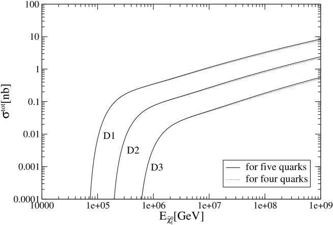
Figure 2: The total cross section of the $s-$channel contributions to $\tilde{\chi}_{1}^{0}-$nucleon scattering for four (dotted curves) and five (solid curves) active quark flavors. The supersymmetric scenarios D1, D2 and D3 are defined in Table 1.

Over most of the parameter space of mSUGRA the lightest neutralino is bino dominated [15, 26]; this is also true for the three scenarios of Table 1. Since the bino coupling to a sfermion is proportional to the hypercharge of that sfermion, a bino–like $\tilde{\chi}_{1}^{0}$ couples predominantly to $SU(2)$ singlet, “right–handed” squarks, whose hypercharges are two (for $\tilde{d}_{R}$) or four (for $\tilde{u}_{R}$) times larger than that of the $SU(2)$ doublet squarks; see Eqs.(5). The total $s-$channel cross section is therefore dominated by the production of $SU(2)$ singlet squarks. Since these squarks do not couple to $SU(2)$ gauginos, they will decay directly into $q+\tilde{\chi}_{1}^{0}$, if the gluino is heavier than these squarks [28]; in mSUGRA this corresponds to $m_{0}\raisebox{-3.69899pt}{~{}\shortstack{$<$ \\ [-0.07cm] $\sim$}}~{}m_{1/2}$. In this case we can approximate the total $s-$channel contribution as production of on–shell squarks which decay back into $q+\tilde{\chi}_{1}^{0}$ final states.

This greatly simplifies the calculation of the cross section differential in the scaling variable $y\equiv 1-E_{\rm out}/E_{\rm in}$, where $E_{\rm in}$ and $E_{\rm out}$ are the incoming and outgoing $\tilde{\chi}_{1}^{0}$ energy in the nucleon rest frame. The crucial observation is that squark decays are isotropic in the squark rest frame, which implies

$$\frac{d\!\sigma_{s}}{d\!\cos\theta^{\ast}}=\frac{\sigma_{s}^{\rm tot}}{2}\,,$$ (7)

where $\theta^{*}$ is the angle between the ingoing and outgoing $\tilde{\chi}_{1}^{0}$ in this frame. In order to get the final expression for the $y$ distribution, we have to boost from the c.m. system into the rest frame of the nucleon. This yields a flat distribution,

$$\frac{d\!\sigma_{s}}{d\!y}=\frac{\sigma_{s}^{\rm tot}}{y_{\rm max}}\,,$$ (8)

where

$$y_{\rm max} = 1-\frac{m^{2}_{\tilde{\chi}_{1}^{0}}}{m^{2}_{\tilde{q}}}\,;$$

$$y_{\rm min} = 0\,.$$ (9)

In the first Eq.(2.1) we have used $\hat{s}=m^{2}_{\tilde{q}}$ for on–shell squark production. Forward scattering in the squark rest frame leads to $E_{\rm out}=E_{\rm in}$, independent of the details of the kinematics; the lower limit for $y$ is therefore always zero. On the other hand, $y=1$, which requires $E_{\rm out}=0$, is possible only for $m_{\tilde{\chi}_{1}^{0}}\rightarrow 0$. Since in mSUGRA $m^{2}_{\tilde{\chi}_{1}^{0}}\ll m^{2}_{\tilde{q}}$, $y_{\rm max}$ is indeed quite close to unity. An LSP will then lose on average about half its energy if it undergoes $s-$channel scattering on a nucleon.

2.2 $t-$channel contribution

We now turn to the calculation of the $t-$channel contribution to the LSP nucleon scattering cross section. As shown in Fig. 3, there are both $W$ (charged current) and $Z$ exchange (neutral current) diagrams; the former produce an outgoing chargino, while the latter have one of the four neutralinos in the final state. There are additional diagrams with antiquarks in both initial and final state, as well as charged current diagrams producing a negative chargino from scattering off a $d$ or $\bar{u}$ quark. Table 2 shows all possible initial and final states, where we again include five active flavors of quarks in the nucleon.

Figure 3: Feynman diagrams for $t-$channel neutralino–nucleon scattering. The arrows indicate the flow of baryon number, and $p_{1,2},\,k_{1,2}$ and $q$ refer to the four–momenta of the initial, final and exchanged particles, respectively.

$W^{\pm}$ exchange				$Z$ exchange
Process			#	Process			#
$\tilde{\chi}_{1}^{0}$		$\tilde{\chi}_{k}^{+}$		$\tilde{\chi}_{1}^{0}$		$\tilde{\chi}_{l}^{0}$
$u$	$\rightarrow$	$d$	$2$	$u$	$\rightarrow$	$u$	$4$
$\tilde{\chi}_{1}^{0}$		$\tilde{\chi}_{k}^{+}$		$\tilde{\chi}_{1}^{0}$		$\tilde{\chi}_{l}^{0}$
$c$	$\rightarrow$	$s$	$2$	$c$	$\rightarrow$	$c$	$4$
$\tilde{\chi}_{1}^{0}$		$\tilde{\chi}_{k}^{-}$		$\tilde{\chi}_{1}^{0}$		$\tilde{\chi}_{l}^{0}$
$\bar{u}$	$\rightarrow$	$\bar{d}$	$2$	$\bar{u}$	$\rightarrow$	$\bar{u}$	$4$
$\tilde{\chi}_{1}^{0}$		$\tilde{\chi}_{k}^{-}$		$\tilde{\chi}_{1}^{0}$		$\tilde{\chi}_{l}^{0}$
$\bar{c}$	$\rightarrow$	$\bar{s}$	$2$	$\bar{c}$	$\rightarrow$	$\bar{c}$	$4$
$\tilde{\chi}_{1}^{0}$		$\tilde{\chi}_{k}^{+}$		$\tilde{\chi}_{1}^{0}$		$\tilde{\chi}_{l}^{0}$
$\bar{d}$	$\rightarrow$	$\bar{u}$	$2$	$\bar{d}$	$\rightarrow$	$\bar{d}$	$4$
$\tilde{\chi}_{1}^{0}$		$\tilde{\chi}_{k}^{+}$		$\tilde{\chi}_{1}^{0}$		$\tilde{\chi}_{l}^{0}$
$\bar{s}$	$\rightarrow$	$\bar{c}$	$2$	$\bar{s}$	$\rightarrow$	$\bar{s}$	$4$
$\tilde{\chi}_{1}^{0}$		$\tilde{\chi}_{k}^{+}$		$\tilde{\chi}_{1}^{0}$		$\tilde{\chi}_{l}^{0}$
$\bar{b}$	$\rightarrow$	$\bar{t}$	$2$	$\bar{b}$	$\rightarrow$	$\bar{b}$	$4$
$\tilde{\chi}_{1}^{0}$		$\tilde{\chi}_{k}^{-}$		$\tilde{\chi}_{1}^{0}$		$\tilde{\chi}_{l}^{0}$
$d$	$\rightarrow$	$u$	$2$	$d$	$\rightarrow$	$d$	$4$
$\tilde{\chi}_{1}^{0}$		$\tilde{\chi}_{k}^{-}$		$\tilde{\chi}_{1}^{0}$		$\tilde{\chi}_{l}^{0}$
$s$	$\rightarrow$	$c$	$2$	$s$	$\rightarrow$	$s$	$4$
$\tilde{\chi}_{1}^{0}$		$\tilde{\chi}_{k}^{-}$		$\tilde{\chi}_{1}^{0}$		$\tilde{\chi}_{l}^{0}$
$b$	$\rightarrow$	$t$	$2$	$b$	$\rightarrow$	$b$	$4$
		$\sum$	$20$			$\sum$	$40$

Table 2: List of processes contributing to $\tilde{\chi}_{1}^{0}-$nucleon scattering through the exchange of an electroweak gauge boson in the $t-$channel, together with the number of different final states. The chargino index $k$ runs from 1 to 2 and the neutralino index $l$ from 1 to 4.

The partonic total cross section can be obtained by integrating over the scattering angle $\theta^{*}$ in the center–of–mass frame; convolution with the relevant quark distribution functions then yields the $t-$channel contribution to the $\tilde{\chi}_{1}^{0}-$nucleon scattering cross section:

$$\sigma_{t}^{\rm tot}(s) = \sum_{q}\int_{x_{\rm min}}^{1}dx\int_{-1}^{\cos\theta^{*}_{\rm max}}d\!\cos\theta^{*}\frac{1}{32\pi}q(x,Q^{2})\frac{|\mathcal{M}|^{2}|\vec{P}^{*}_{2}\left(\hat{s}\right)|}{\hat{s}|\vec{P}_{1}^{*}\left(\hat{s}\right)|}\,,$$ (10)

where $\hat{s}=2xE_{\rm in}m_{N}+m^{2}_{\tilde{\chi}_{1}^{0}}$, and $\vec{P}_{1}^{*}$ and $\vec{P}^{*}_{2}$ are the three–momenta of the incoming and outgoing particles in the c.m. system, respectively. As usually done in deep–inelastic scattering, we identify the scale $Q^{2}$ in the quark distribution functions with the absolute value of the four–momentum $\hat{t}$ exchanged between the participating partons. This causes a minor difficulty: forward scattering ($\cos\theta^{*}=+1$) leads to $Q^{2}=\hat{t}=0$, where the parton distribution functions are not defined. Demanding $Q^{2}>Q^{2}_{\rm min}$ therefore leads to a restriction on the phase space integration:

$$\cos\theta^{*}_{\rm max}=1-\frac{2\hat{s}Q^{2}_{\rm min}}{\left(\hat{s}-m^{2}_{\tilde{\chi}_{1}^{0}}\right)\left(\hat{s}-m^{2}_{\tilde{\chi}_{\rm out}}\right)}\,,$$ (11)

where $\tilde{\chi}_{\rm out}$ stands for the chargino or neutralino in the final state. This in turn affects the lower bound on the momentum fraction $x$:

$$x_{\rm min} = \frac{\frac{1}{2}\left(Q_{\rm min}^{2}+m_{\tilde{\chi}_{\rm out}}^{2}-m_{\tilde{\chi}_{1}^{0}}^{2}\right)+\sqrt{\frac{1}{4}\left(Q^{2}_{\rm min}+m_{\tilde{\chi}_{\rm out}}^{2}+m_{\tilde{\chi}_{1}^{0}}^{2}\right)^{2}-m_{\tilde{\chi}_{\rm out}}^{2}m_{\tilde{\chi}_{1}^{0}}^{2}}}{2E_{\rm in}m_{N}}\,,$$ (12)

where $E_{\rm in}$ is again the energy of the incoming neutralino in the nucleon rest frame. The total cross section depends only very weakly on the choice of $Q_{\min}^{2}$. The $W$ and $Z$ propagators become independent of $Q^{2}=|\hat{t}|$ once $Q^{2}\ll m_{W}^{2}$. Moreover, as we will see shortly, the total cross section is dominated by the production of $\tilde{\chi}_{\rm out}\neq\tilde{\chi}_{1}^{0}$, where $Q_{\rm min}^{2}\ll m^{2}_{\tilde{\chi}_{\rm out}}$ only has a very small effect on $x_{\rm min}$. In our numerical calculations we fixed $Q^{2}_{\rm min}=1$ GeV².

The squared matrix elements $|\mathcal{M}|^{2}$ for the charged current reactions are given by

$$\frac{1}{4}\sum_{\rm spins}|\mathcal{M}|^{2} = \frac{g_{2}^{4}}{\left(\hat{t}-M_{W}^{2}\right)^{2}}\Bigl{[}2|C_{1k}^{L}|^{2}p_{1}\!\cdot\!p_{2}\>k_{1}\!\cdot\!k_{2}+2|C_{1k}^{R}|^{2}p_{1}\!\cdot\!k_{2}\>p_{2}\!\cdot\!k_{1}$$ (13)

$$\hskip 56.9055pt-\left(C_{1k}^{L\ast}C_{1k}^{R}+C_{1k}^{L}C_{1k}^{R\ast}\right)p_{2}\!\cdot\!k_{2}m_{\tilde{\chi}_{k}^{\pm}}m_{\tilde{\chi}_{l}^{0}}\Bigr{]}\,,$$

for the first four cases of Table 2, and

$$\frac{1}{4}\sum_{\rm spins}|\mathcal{M}|^{2} = \frac{g_{2}^{4}}{\left(\hat{t}-M_{W}^{2}\right)^{2}}\bigl{[}2|C_{1k}^{L}|^{2}p_{1}\!\cdot\!k_{2}\>p_{2}\!\cdot\!k_{1}+2|C_{1k}^{R}|^{2}p_{1}\!\cdot\!p_{2}\>k_{1}\!\cdot\!k_{2}$$ (14)

$$\hskip 56.9055pt-\left(C_{1k}^{L\ast}C_{1k}^{R}+C_{1k}^{L}C_{1k}^{R\ast}\right)p_{2}\!\cdot\!k_{2}m_{\tilde{\chi}_{k}^{\pm}}m_{\tilde{\chi}_{l}^{0}}\bigr{]}\,,$$

for the last six cases of Table 2; note that the results (13) and (14) differ by the exchange of the left– and right–handed $W^{\pm}\tilde{\chi}_{1}^{0}\tilde{\chi}_{k}^{\mp}$ couplings. These couplings are given by [24]

$$C_{1k}^{L} = N_{12}\mathcal{V}_{k1}^{\ast}-\frac{1}{\sqrt{2}}N_{14}\mathcal{V}_{k2}^{\ast}\,,$$

$$C_{1k}^{R} = N_{12}^{\ast}\mathcal{U}_{k1}+\frac{1}{\sqrt{2}}N_{13}^{\ast}\mathcal{U}_{k2}\,.$$ (15)

Here, the index $k$ runs from 1 to 2, $\mathcal{U}$ and $\mathcal{V}$ denote the chargino mixing matrices, $m_{\tilde{\chi}_{k}^{\pm}}$ is the mass of the outgoing chargino, and $\hat{t}=-Q^{2}=(k_{1}-p_{1})^{2}$; the four–momenta have been defined in Fig. 3. In Eqs.(13) and (14) we have ignored quark flavor mixing, i.e. we replaced the quark mixing matrix by the unit matrix.

Due to the Majorana nature of the neutralinos, neutral current reactions on a quark and antiquark are described by the same matrix element:

$$\frac{1}{4}\sum_{\rm spins}|\mathcal{M}|^{2} = \frac{2}{c_{W}^{4}}\frac{g_{2}^{4}\left(|g_{L}^{q}|^{2}+|g_{R}^{q}|^{2}\right)}{\left(t-M_{W}^{2}\right)^{2}}\Bigl{[}\left(|N_{l1}^{L}|^{2}+|N_{l1}^{R}|^{2}\right)\left(p_{1}\!\cdot\!p_{2}\>k_{1}\!\cdot\!k_{2}+p_{1}\!\cdot\!k_{2}\>p_{2}\!\cdot\!k_{1}\right)$$ (16)

$$\hskip 96.73918pt-\left(N_{l1}^{L}N_{l1}^{R\ast}+N_{l1}^{R}N_{l1}^{L\ast}\right)p_{2}\!\cdot\!k_{2}m_{\tilde{\chi}_{1}^{0}}m_{\tilde{\chi}_{l}^{0}}\Bigr{]}\,,$$

with

$$c_{W} = \cos\theta_{W}\,,$$

$$N_{l1}^{L} = \frac{1}{2}\left(-N_{l3}N_{13}^{\ast}+N_{l4}N_{14}^{\ast}\right)\,,$$

$$N_{l1}^{R} = -\left(N_{l1}^{L}\right)^{\ast}\,,$$

$$g_{L}^{q} = T_{3,q}-Q_{q}\sin^{2}\theta_{W}\,,$$

$$g_{R}^{q} = Q_{q}\sin^{2}\theta_{W}\,.$$ (17)

The index $l$ in Eqs.(16) and (2.2) runs from $1$ to $4$, and $Q_{q}$ and $T_{3,q}$ have been introduced in Eqs.(5).

Scenario	$m_{\tilde{\chi}_{1}^{0}}$	$m_{\tilde{\chi}_{2}^{0}}$	$m_{\tilde{\chi}_{3}^{0}}$	$m_{\tilde{\chi}_{4}^{0}}$	$m_{\tilde{\chi}_{1}^{+}}$	$m_{\tilde{\chi}_{2}^{+}}$	$GF$ [$\%$]
D2	104	206	468	477	206	476	99.4
D3	189	367	800	805	367	805	99.8
H1	125	137	742	801	130	742	1.2
H2	300	310	940	970	303	970	1.1

Table 3: Neutralino and chargino masses (in GeV) as well as the gaugino fraction $GF=|N_{11}|^{2}+|N_{12}|^{2}$ for the four scenarios discussed in the text. Scenarios D2 and D3, where $\tilde{\chi}_{1}^{0}$ is bino–like, have already been introduced in Table 1, whereas scenarios H1 and H2 describe higgsino–like $\tilde{\chi}_{1}^{0}$; note that the higgsino fraction is $100\%-GF$.

As mentioned earlier, all neutralino and chargino states can be produced in $t-$channel $\tilde{\chi}_{1}^{0}-$nucleon scattering. Table 3 lists the masses of these particles for four scenarios. The first two have already been introduced in Table 1 and describe bino–dominated $\tilde{\chi}_{1}^{0}$ states, whereas in scenarios H1 and H2 $\tilde{\chi}_{1}^{0}$ is dominated by its higgsino components. Eqs.(2.2) and (2.2) show that bino–like states, which have $|N_{12}|,\,|N_{13}|,\,|N_{14}|\ll 1$, have suppressed couplings to gauge bosons. We therefore expect the $t-$channel contributions to be subdominant for the scenarios with bino–like $\tilde{\chi}_{1}^{0}$. This is borne out by Fig. 4, which shows the $s-$ and $t-$channel contributions to the total $\tilde{\chi}_{1}^{0}-$nucleon scattering cross section for the three scenarios of Table 1. The $t-$channel contribution dominates only at low energies, below the threshold for squark production; however, there the cross section is in any case very small, and any possible signal from UHE LSPs will be masked by the much larger neutrino signal. At higher energies the $s-$channel contribution is at least a factor of 30 larger than those from all $t-$channel diagrams. Note that the latter also decrease quickly with increasing sparticle mass scale, i.e. when going from scenario D1 over D2 to D3. The reason is that increasing the gaugino mass parameter $m_{1/2}$ in mSUGRA not only increases the bino mass, via the condition of electroweak symmetry breaking it also increases the absolute value of the higgsino mass. Both effects tend to reduce gaugino–higgsino mixing, and hence the couplings of $\tilde{\chi}_{1}^{0}$ to gauge bosons. These results show that one can indeed ignore all $t-$channel contributions for bino–like LSPs, as done in refs.[17, 18].

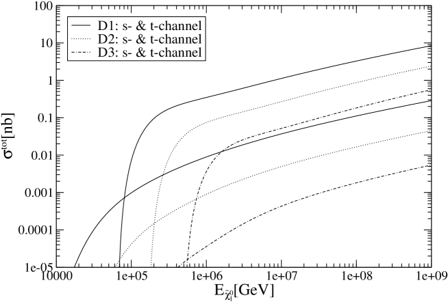
Figure 4: The total $\tilde{\chi}_{1}^{0}-$nucleon scattering cross section for the three scenarios of Table 1, where $\tilde{\chi}_{1}^{0}$ is bino–dominated. At large energies the upper (lower) curves show the contribution from $s-$ ($t-$)channel diagrams. Interference between these diagrams is negligible.

In contrast, Eqs.(5) show that a higgsino–like $\tilde{\chi}_{1}^{0}$, with $|N_{11}|,\,|N_{12}|\ll 1$, has very small couplings to light quarks, which suppresses the $s-$channel contribution, whereas $|N_{13}|,\,|N_{14}|$ are sizable and lead to unsuppressed couplings to gauge bosons. We therefore expect the $t-$channel contributions to dominate the total $\tilde{\chi}_{1}^{0}-$nucleon scattering cross section for higgsino–like $\tilde{\chi}_{1}^{0}$. Fig. 5 shows that this is indeed the case. The solid and dotted curves in this figure show the total $t-$ and $s-$channel contributions in scenarios H1 and H2 of Table 3, where the $t-$channel contributions now correspond to the upper curves. Here we used squark masses of around 1.9 TeV for scenario H2, and about 1 TeV for H1; note that large scalar masses, $m_{\tilde{q}}\gg|\mu|$ are required in mSUGRA if the LSP is to be higgsino–like [15]. For comparison we also show the total cross section for neutrino–nucleon scattering [29] (dot–dashed curve). Since neutrinos are also $SU(2)$ doublets, their cross section is similar to that of higgsino–like neutralinos. However, some differences remain even at high energies. The reason is that the quark distribution functions appearing in the expression (10) for the total $t-$channel contribution to the cross section peak strongly at small $x$. As a result, the partonic cms energy $\sqrt{\hat{s}}$ is often not much larger than the masses of the relevant charginos and neutralinos, leading to some suppression of the LSP cross section relative to the neutrino cross section. We will come back to this point shortly.

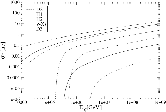
Figure 5: Comparison of total cross sections for neutrinos (dashed-dotted curve) and higgsino– and bino–like $\tilde{\chi}_{1}^{0}$. For scenarios H1 and H2 (see Table 3) with higgsino–like LSP, $t-$ and $s-$channel contributions are shown by the upper and lower curves, respectively; for scenarios D2 and D3, only the dominant $s-$channel contributions are shown.

The dashed and dash–doubledotted curves in Fig. 5 show again the results for scenarios D2 and D3, where we have omitted the subdominant $t-$channel contributions for clarity. We see that these scenarios lead to somewhat smaller total cross sections than the scenarios with higgsino–like LSP. The $s-$channel partonic subprocesses occur at first order in the weak coupling, whereas the $t-$channel diagrams are of second order. However, this relative enhancement of the $s-$channel contributions is over–compensated by the fact that the relevant scale in the partonic $s-$channel cross section is the squark mass, while for the $t-$channel cross sections it is given by the mass of the exchanged gauge boson. On the other hand, comparison with Fig. 4 shows that for scenario D1 with relatively light squarks, the ($s-$channel dominated) cross section is about the same as the ($t-$channel dominated) cross section for higgsino–like LSP.

Scenarios with higgsino–like $\tilde{\chi}_{1}^{0}$ have higgsino mass parameter $|\mu|$ significantly smaller than the $SU(2)_{L}$ and $U(1)_{Y}$ gaugino mass parameters $|M_{2}|$ and $|M_{1}|$. As a result, the second neutralino $\tilde{\chi}_{2}^{0}$ and lighter chargino $\tilde{\chi}_{1}^{\pm}$ will also be higgsino–like, but $\tilde{\chi}_{3}^{0},\,\tilde{\chi}_{4}^{0}$ and $\tilde{\chi}_{2}^{\pm}$ will be gaugino–like. Since gauge bosons can only couple to two higgsinos (or, in case of $W^{\pm}$, to two $SU(2)_{L}$ gauginos), the production of these heavier neutralino and chargino states is strongly suppressed, as shown in Fig. 6. This figure shows that the neutral current reaction with $\tilde{\chi}_{1}^{0}$ in the final state is also suppressed. This is due to the fact that $|N_{13}|\simeq|N_{14}|$ for higgsino–like LSP, leading to a strong cancellation of the $Z\tilde{\chi}_{1}^{0}\tilde{\chi}_{1}^{0}$ couplings in Eqs.(2.2). The total neutral and charged current contributions are therefore dominated by $\tilde{\chi}_{2}^{0}$ and $\tilde{\chi}_{1}^{\pm}$ production, respectively. The $\tilde{\chi}_{1}^{\pm}$ cross section is about two times larger, since $\tilde{\chi}_{2}^{0}$, $\tilde{\chi}_{1}^{+}$ and $\tilde{\chi}_{1}^{-}$ contribute about equally. All three states are essentially $SU(2)$ doublets, and are produced with nearly pure vector coupling, leading to nearly identical cross sections for $\tilde{\chi}_{1}^{\pm}$ production on a quark or antiquark, see Eqs.(13), (14).

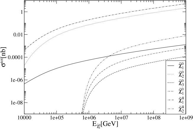
Figure 6: Separate contributions from the four neutralinos and two charginos to the total $t-$channel cross section in scenario H2 of Table 3.

We now turn to a discussion of the $y-$distribution of the $t-$channel contribution. The scaling variable $y$ is related to the scattering angle via

$$y=\left(1-\cos\theta^{*}\right)\frac{\hat{s}-m^{2}_{\tilde{\chi}_{\rm out}}}{2\hat{s}}\,.$$ (18)

The cross section differential in $y$ can therefore be calculated from Eq.(10) by a substitution of variables, and inverting the order of integration:

$$\frac{d\sigma_{t}}{dy} = \sum_{q}\int_{x_{-}}^{1}dxq\!\left(x,Q^{2}\right)\frac{|\mathcal{M}|^{2}}{16\pi(\hat{s}-m^{2}_{\tilde{\chi}_{1}^{0}})}\,.$$ (19)

Eqs.(18) and (11) imply that for given $x$,

$$y\in\left[\frac{Q^{2}_{\rm min}}{2xE_{\rm in}m_{N}},\ 1-\frac{m^{2}_{\tilde{\chi}_{\rm out}}}{\hat{s}}\right]\,.$$ (20)

Using $\hat{s}=m^{2}_{\tilde{\chi}_{1}^{0}}+2xE_{\rm in}m_{N}$, this gives for the lower bound on the $x-$integration in Eq.(19):

$$x_{-}=\frac{1}{2E_{\rm in}m_{N}}\,\max\left(\frac{Q^{2}_{\rm min}}{y},\ \frac{m^{2}_{\tilde{\chi}_{\rm out}}}{1-y}-m^{2}_{\tilde{\chi}_{1}^{0}}\right)\,.$$ (21)

Since $Q^{2}_{\rm min}=1$ GeV${}^{2}\ll m^{2}_{\tilde{\chi}_{1}^{0}}$, for most values of $y$ the lower bound on $x$ is determined by the second term in Eq.(21); the restriction on $Q^{2}$ determines $x_{-}$ only for very small values of $y$.

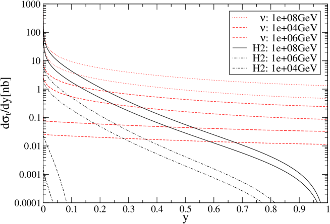
Figure 7: Differential neutral and charged current $t-$channel cross sections $d\sigma/dy$ for LSP–nucleon scattering in scenario H2 (black curves), and for neutrino–nucleon scattering (red or grey curves), for three different energies. The charged current contributions are given by the upper curve for a fixed energy.

Fig. 7 shows the differential cross section $d\sigma/dy$ for scenario H2 and three different energies. The charged and neutral current contributions are shown separately. They have very similar shapes at all energies. This is not surprising, since in the pure higgsino limit, both contributions are from vector–like couplings with equal strength. Moreover, Table 3 shows that the masses of $\tilde{\chi}_{2}^{0}$ and $\tilde{\chi}_{1}^{\pm}$ are very close to each other; we saw in Fig. 6 that the production of these two particles dominates the total $t-$channel contribution.

Fig. 7 also shows the differential cross section for neutrino–nucleon scattering at the same energies. While neutrino and neutralino cross sections are quite similar for $y\ll 1$, the latter fall much more quickly with increasing $y$. This is largely due to the lower bound (21) on the integral over $x$ in Eq.(19), which increases quickly with increasing $y$. Notice that in the region of small $y$, which dominates the total cross section, $x_{-}$ is given by the difference between the masses of the incoming and outgoing $\tilde{\chi}$ particles. Table  3 shows that this difference is smaller for scenario H2, which has much larger masses for the higgsino–like states. This explains why the difference between the total cross sections in scenarios H1 and H2 depicted in Fig. 5 is smaller than that between the cross section for H1 and the neutrino cross section. Scenario H2 still gives a smaller cross section since the mass terms enter the squared matrix elements (13), (14) and (16) with negative sign. The same effect also explains why the ratio of charged and neutral current contributions falls slightly with increasing $y$: the fact that $\tilde{\chi}_{1}^{\pm}$ is slightly lighter than $\tilde{\chi}_{2}^{0}$ is more important at small $y$. In case of neutrinos, $y\rightarrow 1$ remains possible at very small $x$. However, increasing $y$ also means increasing the squared four–momentum exchange $|\hat{t}|$ for fixed $\hat{s}$; this explains the decrease of the neutrino cross sections.

Up to this point we have not considered the interference between the $s-$ and $t-$channel contributions. This is suppressed by two effects. First, it can only occur for outgoing $\tilde{\chi}_{1}^{0}$ state; we saw in Fig. 6 that this final state does not contribute much to the total $t-$channel cross section. Secondly, the interference between the $t-$channel gauge boson and $s-$channel squark propagators vanishes at $\hat{s}=m^{2}_{\tilde{q}}$, where the latter is largest in absolute size, but purely imaginary. Interference can thus only occur for off–shell squark exchange, and is hence of higher order in perturbation theory. These interference contributions can therefore safely be neglected.

3 Solution of the transport equation

We are now ready to discuss the propagation of UHE neutralino LSPs through matter. This is described by so–called transport equations, which have also been used to describe neutrino propagation through the Earth [22, 21, 23]. We will again treat $s-$ and $t-$channel dominated scenarios separately; we saw in the previous Section that this corresponds to scenarios with bino– and higgsino–like LSP, respectively.

3.1 Transport equation for $s-$channel scattering

The quantity we wish to compute is the differential flux $F_{\tilde{\chi}_{1}^{0}}$ as function of the LSP energy $E$ and matter depth $X$, where the latter quantity is customarily given as a column depth, measured in g/cm² or, in natural units, in GeV³; for the Earth, $X\in[0,\,2.398\cdot 10^{6}$ GeV${}^{3}]$ [30]. A UHE LSP interacting with matter at rest can only lose energy. The interactions of LSPs with energy $E$ will therefore always reduce $F_{\tilde{\chi}_{1}^{0}}(E)$. The size of this effect is determined by the interaction length $\lambda_{\tilde{\chi}_{1}^{0}}$, which is given by

$$\lambda_{\tilde{\chi}_{1}^{0}}(E)^{-1}=N_{A}\sigma^{\rm tot}_{\tilde{\chi}_{1}^{0}N}(E)\,,$$ (22)

where $N_{A}=6.022\times 10^{23}\mbox{~{}g}^{-1}$ is Avogadro’s number, and in the given scenario $\sigma^{\rm tot}_{\tilde{\chi}_{1}^{0}N}\simeq\sigma^{\rm tot}_{s}$ of Eq.(3). On the other hand, $F_{\tilde{\chi}_{1}^{0}}(E)$ can be increased by the interactions of LSPs with energy $E_{y}\equiv E/(1-y)>E$ losing a fraction $y$ of their energy. These considerations lead to the transport equation

$$\frac{\partial F_{\tilde{\chi}_{1}^{0}}(E,X)}{\partial X} = -\frac{F_{\tilde{\chi}_{1}^{0}}(E,X)}{\lambda_{\tilde{\chi}_{1}^{0}}(E)}+\frac{1}{\lambda_{\tilde{\chi}_{1}^{0}}(E)}\int_{0}^{y_{\rm max}}\frac{dy}{1-y}K_{s}(E,y)F_{\tilde{\chi}_{1}^{0}}(E_{y},X)\,,$$ (23)

where the kernel is determined by the differential cross section given in Eq.(8):

$$K_{s}(E,y) = \frac{1}{\sigma^{\rm tot}_{s}(E)}\frac{d\sigma_{s}(E_{y})}{dy}\,,$$ (24)

and $y_{\rm max}$ has been given in Eq.(2.1). Note that Eq.(23) assumes collinear kinematics, where the produced LSP goes in the same direction as the original one. This is justified for ultra–relativistic LSPs, whose scattering angle is $\theta\raisebox{-3.69899pt}{~{}\shortstack{$<$ \\ [-0.07cm] $\sim$}}~{}m_{\tilde{q}}/E_{\rm in}\raisebox{-3.69899pt}{~{}\shortstack{$<$ \\ [-0.07cm] $\sim$}}~{}10^{-3}$ for energies of interest.

An important property of $\tilde{\chi}_{1}^{0}-$nucleon scattering is that it always produces another $\tilde{\chi}_{1}^{0}$ in the final state. The total flux,

$$\Phi_{\tilde{\chi}_{1}^{0}}=\int_{m_{\tilde{\chi}_{1}^{0}}}^{E_{\rm max}}F_{\tilde{\chi}_{1}^{0}}(E,X)dE\,,$$ (25)

must therefore remain constant, independent of $X$; here $E_{\rm max}$ is the maximal $\tilde{\chi}_{1}^{0}$ energy, beyond which the incident LSP flux vanishes. This is reflected in the fact that integrating the right–hand side of Eq.(23) over the energy gives zero, i.e. $d\Phi_{\tilde{\chi}_{1}^{0}}/dX=0$. This allows an important check of the procedure used to solve the transport equation.

The standard method to solve the analogous transport equation for neutrinos is based on an iteration [22, 21, 23]. It uses an effective interaction length $\Lambda_{\tilde{\chi}_{1}^{0}}$ defined by

$$F_{\tilde{\chi}_{1}^{0}}(E,X)=F_{\tilde{\chi}_{1}^{0}}(E,0)\exp\left[-\frac{X}{\Lambda_{\tilde{\chi}_{1}^{0}}(E,X)}\right]\,,$$ (26)

which in turn leads to the definition of a “$Z-$factor”:

$$\Lambda_{\tilde{\chi}_{1}^{0}}(E,X)=\frac{\lambda_{\tilde{\chi}_{1}^{0}}(E)}{1-Z_{\tilde{\chi}_{1}^{0}}(E,X)}\,.$$ (27)

The transport equation can then be re–written as an integral equation for $Z_{\tilde{\chi}_{1}^{0}}$. This equation can be solved iteratively, starting from the $0-$th order ansatz $Z^{(0)}_{\tilde{\chi}_{1}^{0}}=0$. This treatment was first introduced in ref.[22] to describe the propagation of electron and muon neutrinos. In this case the iteration converges fast, so that the first non–trivial solution $Z^{(1)}_{\nu_{\mu}}$ deviates by at most 4% from the final answer. The same first–order solution was then used in refs.[21, 23] to describe $\nu_{\tau}$ propagation. We therefore tried to use it for LSP propagation as well.

Unfortunately we found that the first–order solution badly violates flux conservation in our case. A close reading of ref.[22] shows that this is actually not very surprising. To begin with, the $0-$th order solution evidently ignores regeneration completely. Flux conservation requires that the differential flux must increase for some range of energies; Eqs.(26) and (27) show that this is possible only if the $Z-$factor exceeds unity, which means that the effective interaction length $\Lambda$ must become negative. This did not happen in ref.[22], since charged current reactions of electron or muon neutrinos effectively lead to a loss of this neutrino, thereby reducing the total neutrino flux. Flux conservation was therefore of no concern in ref.[22]. Moreover, the neutral current reaction, whose regeneration effect was included in this treatment, has $d\sigma/dy$ quite strongly peaked at low $y$, see Fig. 7. According to ref.[22], this accelerates the convergence of the iteration. However, in our case $d\sigma_{s}/dy$ is flat, see Eq.(8). It is therefore not surprising that this algorithm does not work very well in our case.

We therefore use a straightforward numerical solution of the transport equation (23), based on the first order Taylor expansion:

$$F_{\tilde{\chi}_{1}^{0}}(E,X+dX)=F_{\tilde{\chi}_{1}^{0}}(E,X)+dX\frac{\partial F_{\tilde{\chi}_{1}^{0}}(E,X)}{\partial X}+\cdots\,.$$ (28)

We found that a more sophisticated algorithm, e.g. the Runge–Kutta method, does not offer much of an advantage in terms of accuracy achieved for a fixed CPU time spent. We parameterize $F_{\tilde{\chi}_{1}^{0}}(E)$ for given $X$ as cubic spine. The one–dimensional integral appearing in Eq.(23) can then be evaluated using, e.g., the Simpson method.

Since the transport equation is a first order differential equation, we have to specify the boundary condition $F_{\tilde{\chi}_{1}^{0}}(E,0)$. We use three different ansätze:

$$\textrm{Spectrum \ 1:}\hskip 2.84544ptF_{\tilde{\chi}_{1}^{0}}^{0}(E,0) = N_{1}E^{-2}F_{\rm cut}(E)\,;$$

$$\textrm{Spectrum \ 2:}\hskip 2.84544ptF_{\tilde{\chi}_{1}^{0}}^{0}(E,0) = N_{2}E^{-1.5}F_{\rm cut}(E)\,;$$

$$\textrm{Spectrum \ 3:}\hskip 2.84544ptF_{\tilde{\chi}_{1}^{0}}^{0}(E,0) = N_{3}E^{-1}\frac{1}{\left(1+\frac{E}{10^{8}\ {\rm GeV}}\right)^{2}}F_{\rm cut}(E)\,,$$ (29)

where the $N_{i}$ are arbitrary normalization factors. The first two ansätze would yield an infinite total energy stored in LSPs, had we not introduced a cut–off function

$$F_{\rm cut}(E)=1-\left(\frac{E}{E_{\rm cut}}\right)^{4}\,,$$ (30)

with $F_{\rm cut}(E)=0$ for $E>E_{\rm cut}$. In top–down scenarios, $E_{\rm cut}$ should be $\sim M_{X}/2$. In our numerical examples we instead use $E_{\rm cut}=10^{9}$ GeV. We will see below that LSPs with initial energy $E>10^{9}$ GeV will interact very soon, i.e. the flux at $E>10^{9}$ GeV will quickly become negligible. Due to the shorter interaction length, choosing $E_{\rm cut}>10^{9}$ GeV would greatly increase the numerical cost of the solution. On the other hand, this relatively small value of $E_{\rm cut}\ll M_{X}$ is justified if neutralinos with $E>E_{\rm cut}$ contribute negligibly to the total LSP flux impinging on Earth, which is often the case [11].

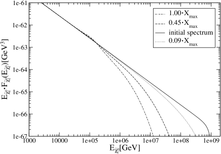
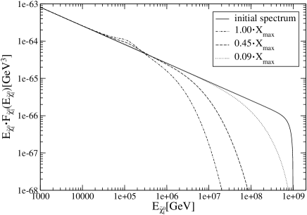
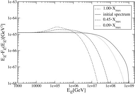
Figure 8: Modification of our three LSP spectra due to propagation through the Earth for scenario D1 with bino–like LSP. The solid curve shows the initial spectra (in arbitrary units), and the dotted, dot–dashed and dashed curves show the flux after a column depth of $0.09X_{\rm max},\,0.45X_{\rm max}$ and $X_{\rm max}=2.4\cdot 10^{6}$ GeV³. The top–left, top–right and bottom frames are for Spectrum 1, Spectrum 2 and Spectrum 3 of Eqs.(3.1), respectively.

In this Subsection we focus on the first scenario of Table 1. We saw in Fig. 2 that this leads to the largest cross section, and hence the largest propagation effects. Results for the three initial fluxes of Eq.(3.1) are shown in Fig. 8. The initial spectrum should get reduced significantly once the traversed column depth exceeds the interactions length; note that according to Eq.(22), $\sigma^{\rm tot}_{\tilde{\chi}_{1}^{0}N}=1$ nb corresponds to an interaction length $\lambda_{\tilde{\chi}_{1}^{0}}\simeq 0.36\cdot 10^{6}$ GeV${}^{3}\simeq 0.15X_{\rm max}$. Fig. 2 shows that in scenario D1 this cross section is reached at $E_{\rm in}\simeq 10^{7}$ GeV. We see in the two upper frames of Fig. 8 that the suppression of the LSP spectrum indeed begins to be noticeable around that energy for $X=0.09X_{\rm max}$.

In the lower frame the suppression starts at somewhat higher energy for this small column depth, since for this very hard initial spectrum the regeneration effect is maximized. This effect creates a bump in the spectrum. The peak of the bump is at an energy such that the interaction length is slightly larger than the traversed column depth; since the cross section rises with energy, the bump shifts to lower energies with increasing column depth. Conservation of the total flux (3.1) implies that this bump is more noticeable for a harder initial spectrum. An analogous argument explains why the energy where the spectrum begins to be suppressed becomes smaller with increasing column depth. This can also be understood from the simple observation that increasing column depth increases the probability for interactions between LSPs and matter.

Fig. 2 shows that at high energies, the total $s-$channel cross section for bino–like LSP is roughly proportional to $(1/m^{2}_{\tilde{q}})(E_{\rm in}/m_{\tilde{q}})^{0.4}$. According to Table 1, squarks are about 2.7 times heavier in scenario D3 than in scenario D1. The onset of the suppression of the initial LSP spectrum, and the location of the bump produced by regeneration, will thus occur at about 12 times higher energy than in scenario D1.

As discussed at the beginning of this Subsection, the total LSP flux (25) must be conserved. We checked that our numerical solution satisfies this constraint very well, with maximal deviation of less than 0.1% even for the hardest spectrum and largest column depth. In contrast, for the hardest incident LSP spectrum the prediction of the first–order iterative solution can violate flux conservation by a factor of two or more.

3.2 Transport equation for $t-$channel scattering

We consider the transport equation for $t-$channel scattering only for a scenario with higgsino–dominated LSP; Fig. 4 showed that $t-$channel contributions are negligible for a bino–like neutralino. As in case of neutrinos [22, 21, 23], there are both charged and neutral current contributions. We saw in Fig. 6 that these predominantly lead to the production of $\tilde{\chi}_{1}^{\pm}$ and $\tilde{\chi}_{2}^{0}$, respectively. Here we will ignore the contribution from all other final states; this approximation is good at the few % level.

In case of $\nu_{\tau}$ propagation [21, 23] one usually writes two coupled transport equations, for $\nu_{\tau}$ itself and for the $\tau$ leptons produced in $\nu_{\tau}$ charged current reactions. Correspondingly we would need three coupled transport equations in our case, describing the spectra of $\tilde{\chi}_{1}^{0},\,\tilde{\chi}_{1}^{\pm}$ and $\tilde{\chi}_{2}^{0}$. However, these heavier produced particles decay well before they lose a significant fraction of their energy through interactions. This is true even for $\tau$ leptons of the relevant energy; the $\tilde{\chi}_{1}^{\pm}$ and $\tilde{\chi}_{2}^{0}$ states in the scenarios of interest have much shorter lifetimes [by a factor of order $(m_{\tilde{\chi}_{\rm out}}-m_{\tilde{\chi}_{1}^{0}})^{5}/m_{\tau}^{5}$], and significantly shorter decay lengths for a given lifetime (due to their larger masses, i.e. smaller $\gamma$ factors). $t-$channel scattering can thus be treated through an integration kernel in the transport equation which is computed from a convolution of the $\tilde{\chi}_{\rm out}$ production and decay spectra. We treat charged and neutral current contributions separately:

$$\frac{\partial F_{\tilde{\chi}_{1}^{0}}(E,X)}{\partial X} = -\frac{F_{\tilde{\chi}_{1}^{0}}(E,X)}{\lambda_{\tilde{\chi}_{1}^{0}}(E)}+\frac{1}{\lambda_{\tilde{\chi}_{1}^{0}}(E)}\int_{0}^{1}\frac{dy}{1-y}K_{\tilde{\chi}_{1}^{0}}^{NC}(E,y)F_{\tilde{\chi}_{1}^{0}}(E_{y},X)$$ (31)

$$+\frac{1}{\lambda_{\tilde{\chi}_{1}^{0}}(E)}\int_{0}^{1}\frac{dy}{1-y}K_{\tilde{\chi}_{1}^{0}}^{CC}(E,y)F_{\tilde{\chi}_{1}^{0}}(E_{y},X)\,,$$

where the interaction length $\lambda_{\tilde{\chi}_{1}^{0}}$ has been given by Eq.(22). The structure of the equation is very similar to Eq.(23) describing $s-$channel scattering. The integration kernels are most easily written as convolutions in the variable $z=1-y=E_{\rm out}/E_{\rm in}$:

$$K_{\tilde{\chi}_{1}^{0}}^{NC,CC}(E,y) = \frac{1}{\sigma_{t}(E)}\int_{z_{1,{\rm min}}}^{z_{1,{\rm max}}}d\!z_{1}\int_{z_{2,{\rm min}}}^{z_{2,{\rm max}}}d\!z_{2}\delta\!\left(z-z_{1}z_{2}\right)\frac{d\sigma^{NC,CC}(E_{y},z_{1})}{dz_{1}}\left.\frac{1}{\Gamma}\frac{d\Gamma(z_{1}E_{y},z_{2})}{dz_{2}}\right|_{y=1-z}$$

$$= \frac{1}{\sigma_{t}(E)}\int_{z}^{z_{1,{\rm max}}}\frac{d\!z_{1}}{z_{1}}\frac{d\sigma^{NC,CC}(E_{y},z_{1})}{dz_{1}}\left.\frac{1}{\Gamma}\frac{d\Gamma(z_{1}E_{y},\frac{z}{z_{1}})}{dz_{2}}\theta(z-z_{\rm min})\theta(z_{\rm max}-z)\right|_{y=1-z}\,.$$

The limits $z_{1,{\rm min,\,max}}$ for the outer integration in the first line of Eq.(3.2) follow from Eq.(20) with $x\rightarrow 1$, i.e. $\hat{s}\rightarrow s=2E_{y}m_{N}+m_{\tilde{\chi}_{1}^{0}}^{2}$. The limits for the inner integration follow from $\tilde{\chi}_{\rm out}$ decay kinematics described below. The $\theta-$functions in the second line of Eq.(3.2) ensure that $y$ lies within the kinematical limits, with $z_{\rm min}=z_{1,{\rm min}}z_{2,{\rm min}}$ and $z_{\rm max}=z_{1,{\rm max}}z_{2,{\rm max}}$. Note that both integration kernels in Eq.(31) are normalized to the total $\tilde{\chi}_{1}^{0}-$nucleon scattering cross section, which is here approximated by the $t-$channel contribution given by Eq.(10). Finally, Eq.(31) again assumes collinear kinematics, where the LSP produced in $\tilde{\chi}_{\rm out}$ decay goes into the same direction as the original LSP.

The missing piece in Eq.(3.2) is the differential decay spectrum of the produced $\tilde{\chi}_{\rm out}$. Due to the small $\tilde{\chi}_{\rm out}-\tilde{\chi}_{1}^{0}$ mass difference for higgsino–like LSP, see Table 3, we only need to consider three–body decays, $\tilde{\chi}_{\rm out}\rightarrow\tilde{\chi}_{1}^{0}f_{1}f_{2}$, where $f_{1},\,f_{2}$ are two SM (anti)fermions whose masses we neglect. In the $\tilde{\chi}_{\rm out}$ rest frame we then have:

$$\frac{d\Gamma}{dE^{*}_{\tilde{\chi}_{1}^{0}}}=\frac{1}{8m_{\tilde{\chi}_{\rm out}}\left(2\pi\right)^{3}}\int_{E_{f,{\rm min}}^{*}}^{E_{f,{\rm max}}^{*}}dE_{f}^{*}|{\cal M}|^{2}\,,$$ (33)

where $E_{f}^{*}$ is the energy of one of the two massless (anti)fermions (the energy of the other being determined by energy conservation). The integration limits in Eq.(33) are given by

$$E_{f\stackrel{{\scriptstyle\rm min}}{{\rm\scriptscriptstyle{max}}}}^{*}=\frac{2m_{\tilde{\chi}_{\rm out}}E^{*}_{\tilde{\chi}_{1}^{0}}-m_{\tilde{\chi}_{1}^{0}}^{2}-m_{\tilde{\chi}_{\rm out}}^{2}}{2E_{\tilde{\chi}_{1}^{0}}^{*}-2m_{\tilde{\chi}_{\rm out}}\pm 2\sqrt{E_{\tilde{\chi}_{1}^{0}}^{*2}-m_{\tilde{\chi}_{1}^{0}}^{2}}}\,.$$ (34)

The total $\tilde{\chi}_{\rm out}$ decay width $\Gamma$ appearing in Eq.(3.2) can be obtained by integrating Eq.(33) over $E^{*}_{\tilde{\chi}_{1}^{0}}$, the lower and upper integration limit being given by $m_{\tilde{\chi}_{1}^{0}}$ and $(m_{\tilde{\chi}_{1}^{0}}^{2}+m^{2}_{\tilde{\chi}_{\rm out}})/(2m_{\tilde{\chi}_{\rm out}})$, respectively.

In order to boost into the frame where $\tilde{\chi}_{\rm out}$ has energy energy $E_{\tilde{\chi}_{\rm out}}$, we have to know the angular distribution of the produced $\tilde{\chi}_{1}^{0}$ in the $\tilde{\chi}_{\rm out}$ rest frame relative to the $\tilde{\chi}_{\rm out}$ flight direction. Here we assume an isotropic distribution, which is appropriate for an unpolarized $\tilde{\chi}_{\rm out}$, and also if $\tilde{\chi}_{\rm out}$ decays via a pure vector coupling; we saw in Subsec. 2.2 that the relevant couplings are indeed almost pure vector couplings in scenarios with higgsino–like LSP. This yields

$$\frac{d\Gamma}{dE_{\tilde{\chi}_{1}^{0}}}=\int_{E^{*}_{\tilde{\chi}_{1}^{0},{\rm min}}}^{E^{*}_{\tilde{\chi}_{1}^{0},{\rm max}}}d\!E_{\tilde{\chi}_{1}^{0}}^{*}\frac{m_{\tilde{\chi}_{\rm out}}}{E_{\tilde{\chi}_{\rm out}}}\frac{1}{\beta\sqrt{E_{\tilde{\chi}_{1}^{0}}^{*2}-m_{\tilde{\chi}_{1}^{0}}^{2}}}\frac{1}{16m_{\tilde{\chi}_{\rm out}}\left(2\pi\right)^{3}}\int_{E_{f,{\rm min}}^{*}}^{E_{f,{\rm max}}^{*}}dE_{f}^{*}|\mathcal{M}|^{2}\,.$$ (35)

The limits for the inner integration in Eq.(35) have been given in Eq.(34), and the limits for the outer integration are:

$$E^{*}_{\tilde{\chi}_{1}^{0},{\rm min}} = \gamma\left(E_{\tilde{\chi}_{1}^{0}}-\beta\sqrt{E^{2}_{\tilde{\chi}_{1}^{0}}-m^{2}_{\tilde{\chi}_{1}^{0}}}\right)\,,$$

$$E^{*}_{\tilde{\chi}_{1}^{0},{\rm max}} = \frac{m^{2}_{\tilde{\chi}_{\rm out}}+m^{2}_{\tilde{\chi}_{1}^{0}}}{2m_{\tilde{\chi}_{\rm out}}}\,.$$ (36)

Here, and in Eq.(35), $\gamma=1/\sqrt{1-\beta^{2}}=E_{\tilde{\chi}_{\rm out}}/m_{\tilde{\chi}_{\rm out}}$. Notice that $E^{*}_{\tilde{\chi}_{1}^{0},{\rm min}}$ reduces to the absolute kinematical minimum of $m_{\tilde{\chi}_{1}^{0}}$ for $E_{\tilde{\chi}_{1}^{0}}=\gamma m_{\tilde{\chi}_{1}^{0}}$, whereas $E^{*}_{\rm max}$ is always determined from the $\tilde{\chi}_{\rm out}$ decay kinematics, independent of $E_{\tilde{\chi}_{1}^{0}}$. Finally, in the relevant limit $\gamma\gg 1$ the limits on the energy $E_{\tilde{\chi}_{1}^{0}}$ of the LSP produced in $\tilde{\chi}_{\rm out}$ decay are

$$E_{\tilde{\chi}_{1}^{0},{\rm min}} = \frac{\gamma\left[m_{\tilde{\chi}_{1}^{0}}^{2}+m_{\tilde{\chi}_{\rm out}}^{2}-\beta\left(m_{\tilde{\chi}_{\rm out}}^{2}-m_{\tilde{\chi}_{1}^{0}}^{2}\right)\right]}{2m_{\tilde{\chi}_{\rm out}}}\longrightarrow\gamma\frac{m^{2}_{\tilde{\chi}_{1}^{0}}}{m_{\tilde{\chi}_{\rm out}}}\,,$$

$$E_{\tilde{\chi}_{1}^{0},{\rm max}} = \frac{\gamma\left[m_{\tilde{\chi}_{1}^{0}}^{2}+m_{\tilde{\chi}_{\rm out}}^{2}+\beta\left(m_{\tilde{\chi}_{\rm out}}^{2}-m_{\tilde{\chi}_{1}^{0}}^{2}\right)\right]}{2m_{\tilde{\chi}_{\rm out}}}\longrightarrow\gamma m_{\tilde{\chi}_{\rm out}}=E_{\tilde{\chi}_{\rm out}}\,.$$ (37)

Since the heavier higgsinos $\tilde{\chi}_{\rm out}$ have very similar masses as the LSP, see Table 3, the energy loss in the $\tilde{\chi}_{\rm out}$ decay process cannot be very large, and may be zero. For example, in scenario H2 the maximal energy loss is 6.7% in $\tilde{\chi}_{2}^{0}$ decays produced in neutral current events, and just 2% in $\tilde{\chi}_{1}^{\pm}$ decays produced in charged current events. For simplicity we therefore treated these decays with purely kinematical decay distributions, i.e. we used a constant matrix element ${\cal M}$ in Eqs.(33) and (35).

Our results for scenario H2 with a higgsino–like LSP are displayed in Fig. 9. Although comparison of Figs. 4 and 5 shows that this scenario and the scenario D1 with bino–like LSP lead to similar total $\tilde{\chi}_{1}^{0}-$nucleon scattering cross sections, comparison of Figs. 8 and 9 shows that the spectrum of higgsino–dominated LSPs is modified much less by propagation effects. The reason is that the $t-$channel exchange contributions have a far steeper $y-$distribution, cf. Fig. 7. The spectrum will be modified significantly only once a given LSP loses a sizable fraction of its energy through interactions. The characteristic length for this is better characterized by $\lambda_{\tilde{\chi}_{1}^{0}}^{\rm eff}\equiv\lambda_{\tilde{\chi}_{1}^{0}}/\langle y\rangle$ than by the interaction length $\lambda_{\tilde{\chi}_{1}^{0}}$ itself. Here $\langle y\rangle$ is the average relative energy loss in an interaction and, for the $t-$channel, subsequent $\tilde{\chi}_{\rm out}$ decay; numerically, $\langle y\rangle\simeq 0.5$ for scenario D1, whereas $\langle y\rangle\simeq 0.07$ for scenario H2. $\lambda_{\tilde{\chi}_{1}^{0}}^{\rm eff}$ therefore differs by about a factor of 10 between scenarios D1 and H2. As a result, even after traversing the whole Earth in scenario H2 only the spectrum at $E\raisebox{-3.69899pt}{~{}\shortstack{$>$ \\ [-0.07cm] $\sim$}}~{}10^{8}$ GeV is suppressed, whereas in scenario D1 with bino–like LSP the suppression already starts at $E\sim 10^{6}$ GeV. The same effect also explains the reduced size of the “regeneration bump” in the spectrum of higgsino–like LSPs. Indeed, for the steepest input spectrum (top–left frame) this feature is no longer visible; however, Table 4 shows that flux conservation is satisfied also in this case. We should mention here that due to the additional integrations required in Eqs.(3.2) and (35), this scenario is numerically much more time consuming than the case of a bino–like LSP.

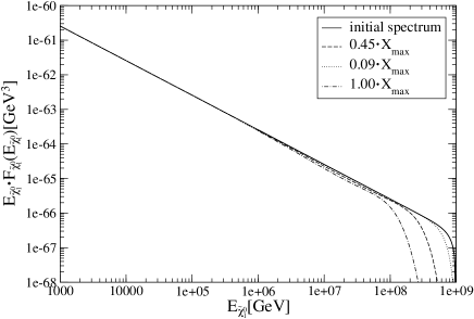
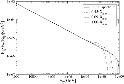
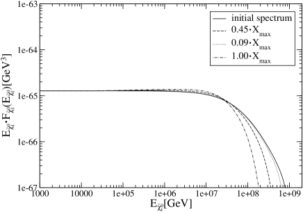
Figure 9: Modification of our three LSP spectra due to propagation through the Earth for scenario H2 with higgsino–like LSP. Conventions are as in Fig. 8.

	$\Phi_{\tilde{\chi}_{1}^{0}}(X)/\Phi_{\tilde{\chi}_{1}^{0}}(0)$
$X/X_{\rm max}$	Spectrum 1	Spectrum 2	Spectrum 3
0.09	1.001	1.000	1.003
0.45	1.001	1.001	1.013
1.	1.001	1.002	1.022

Table 4: Test of conservation of the total LSP flux (25) for the three incident spectra defined in Eqs.(3.1) using scenario H2 with higgsino–like LSP; the LSP spectra are integrated between $10^{3}$ GeV and $E_{\rm cut}=10^{9}$ GeV. The column depths are in units of the maximal Earth column depth $X_{\rm max}=2.4\cdot 10^{6}$ GeV³.

4 Summary and conclusions

The detection of ultra relativistic cosmic neutralinos $\tilde{\chi}_{1}^{0}$ would be a crucial test of both “top-down” models and supersymmetry. This should in principle be feasible by using the Earth to filter out very energetic neutrinos, which would otherwise form an unsurmountable background. In order to assess the prospects of future or planned experiments such as EUSO [31] and OWL [32] a realistic treatment of the interactions of neutralinos with ordinary matter is essential. In this paper we provide two important ingredients of this treatment: an improved calculation of the LSP–nucleon scattering cross section, and a reliable treatment of propagation effects by means of transport equations.

The calculation of the most important contributions to the $\tilde{\chi}_{1}^{0}-$nucleon scattering cross sections are presented in Sec. 2. New features include the calculation of the cross section differential in the energy of the outgoing neutralino, which is needed for the quantitative description of neutralino propagation through the Earth, and a first calculation of $t-$channel scattering processes, which dominate in case of higgsino–like LSP but are negligible for bino–like LSP. We also calculated the contribution from $\tilde{\chi}_{1}^{0}+g\rightarrow\tilde{t}+\bar{t}$, see the Appendix. This process turns out to be sub–dominant in the scenarios we studied, but might be important in special scenarios where the lighter scalar top $\tilde{t}_{1}$ is much lighter than the other squarks. We found that the total cross sections for bino– and higgsino–like LSPs are comparable to each other if first and second generation squark masses are around 400 GeV. For lighter (heavier) squarks the cross section for bino–like LSPs will be enhanced (suppressed). The cross section for higgsino–like LSP is much less dependent on the values of various parameters appearing in the SUSY Lagrangian, as long as the LSP is indeed higgsino–like; at high energies it is only a factor $\sim 1.5$ below the cross section for neutrino–nucleon scattering.

However, the shape of the distribution in the energy loss variable $y$ is quite different in the three cases. Under the assumption that squarks are lighter than gluinos, a bino–like LSP has a flat $y-$distribution, with average $\langle y\rangle\simeq 0.5$. In case of neutrinos, the $y$ distribution peaks at $y=0$, but falls only gently as $y\rightarrow 1$, with $\langle y\rangle\simeq 0.25$ [30, 29]. Finally, higgsino–like neutralinos have a rapidly falling $y-$distribution, with $\langle y\rangle\simeq 0.07$ even after including the energy lost in the decay of the heavier neutralinos and charginos that are produced in this case; note that $t-$channel scattering predominantly produces the other higgsino–like states, whose masses are however very similar to that of the LSP, so that the energy lost in the decay only amounts to a few %. If squarks are lighter than gluinos, most produced squarks decay into a gluino (rather than an LSP) plus a quark, with the gluino decaying into at least three particles (including an LSP again). This would lead to significantly larger energy loss, i.e. $\langle y\rangle$ would be even larger. This case has yet to be analyzed in detail. Here one could use the formalism we developed to treat the decay of the heavier higgsino–like states, although in case of gluinos the decay might proceed over several intermediate states [28].

The transport equation describing LSP propagation through the Earth are discussed in Sec. 3. We first tried the first order iterative solution of ref.[22], but found that it leads to large violations of flux conservation in our case; we suspect that this is also true for the rather similar case of $\nu_{\tau}$ propagation, where the same method was used in [21, 23]. We therefore solved the transport equation by straightforward numerical integration. We found that the $y-$distribution is crucial for understanding the effects of propagation. Indeed, the product of cross section and $\langle y\rangle$ is a much more reliable “figure of merit” here than the cross section itself. In particular, we saw that propagation effects in a scenario with higgsino–like LSP are much milder than in a scenario with bino–like LSP, which has similar total cross section $\sigma$ but much larger $\sigma\langle y\rangle$; in the former case the LSP flux is suppressed only for $E\raisebox{-3.69899pt}{~{}\shortstack{$>$ \\ [-0.07cm] $\sim$}}~{}10^{8}$ GeV, whereas in the latter, the onset of suppression is at $E\simeq 10^{6}$ GeV. Of course, the smaller $\langle y\rangle$ of higgsino–like LSPs also implies that the visible energy released by LSP scattering in or near a detector is much smaller than for a bino–like LSP of equal energy. The visible spectrum for higgsino–like LSPs emerging vertically out of the Earth would nevertheless extend to at least an order of magnitude higher energies than that of bino–like LSPs, for similar total cross section.

Note also that the effective $\langle y\rangle$ for $\nu_{\tau}$ interactions, including the effect of $\tau$ decays, is about 0.55, similar to the case of bino–like LSP. Hence propagation effects will deplete the $\nu_{\tau}$ spectrum much faster than the spectrum of higgsino–like LSPs. We therefore expect that UHE higgsino–like LSPs, which have not yet been considered in the literature, could also yield a viable signal for visible energies roughly between $10^{5}$ and $10^{7}$ GeV. However, a detailed investigation of signals is beyond the scope of this paper. In the analysis of possible signatures for ultra–relativistic higgsino–like LSPs, the finite flight path of the heavier higgsino–like states may also have to be taken into account for scenarios with mass splitting to the LSP below $\sim 2$ GeV.

In this paper we did not discuss the possibility of a wino–like LSP, as in scenarios with anomaly mediated supersymmetry breaking [15]. In this case we expect a strongly suppressed $t-$channel neutral current contribution, since a neutral wino does not couple to $Z$ bosons, but somewhat enhanced charged current contribution, since the wino is an $SU(2)$ triplet rather than a doublet. However, the produced chargino may now lose a significant amount of energy before decaying, since the mass splitting to the LSP if typically only a few hundred MeV in this case, leading to a lifetime which is much longer than that of the $\tau$ lepton. The propagation of these charginos would then have to be described by a second, coupled, transport equation. A wino–like LSP can also have a sizable $s-$channel contribution to the cross section, if squarks are not too heavy. In this case left handed, $SU(2)$ doublet, squarks would be produced predominantly; if lighter than gluinos, these squarks would decay into charged or neutral winos, i.e. into the LSP or the lighter chargino.

In summary, we provided a treatment of the interactions of ultra–relativistic higgsino– or bino–like neutralinos with matter, calculating both the total cross section and the energy lost in these interactions. We also developed a new method to solve the transport equations describing the passage of these neutralinos through matter. This will allow improved estimates of the prospects of future experiments to observe these neutralinos in potentially realistic supersymmetric scenarios. Such an observation would help to solve the forty year old puzzle posed by the cosmic rays at ultra–high energies.

Acknowledgments

We thank Jon Pumplin for correspondence regarding parameterized parton distribution functions. MD thanks the high energy theory group of the University of Hawaii at Manoa for hospitality.

Appendix A Top $+$ stop production

Figure 10: Feynman diagrams contributing to $\tilde{\chi}_{1}^{0}+g\rightarrow\tilde{t}+\bar{t}$. The arrows indicate the flow of baryon number. The diagrams for $\tilde{\chi}_{1}^{0}+g\rightarrow\bar{\tilde{t}}+t$ can be obtained by reversing the directions of these arrows.

The Feynman diagrams for top $+$ stop production via $\tilde{\chi}_{1}^{0}-$gluon fusion are shown in Fig. 10. Here, $p_{i}$, $k_{j}$ are four–momenta in the initial and final state, respectively, and $q_{1}=p_{2}-k_{2}$ and $q_{2}=p_{1}-k_{2}$ are the exchanged four–momenta in the two diagrams. The total squared partonic production amplitude is then given by $|{\cal M}_{a}+{\cal M}_{b}|^{2}=|{\cal M}_{a}|^{2}+|{\cal M}_{b}|^{2}+{\cal M}_{a}{\cal M}_{b}^{\ast}+{\cal M}_{a}^{\ast}{\cal M}_{b}$. In the following we list these three contributions separately.

$|{\cal M}_{a}|^{2}$ term:

$$\frac{1}{4}\sum_{\rm spins}\sum_{\rm colors}|{\cal M}_{a}|^{2} = -\frac{1}{2}\frac{g_{s}^{2}}{\left(t-m_{t}^{2}\right)^{2}}\cdot$$ (38)

$$\mbox{}\cdot\biggl{[}-\left(|G_{i}^{L}|^{2}+|G_{i}^{R}|^{2}\right)\left(k_{2}\cdot q_{1}\>p_{1}\cdot q_{1}-k_{2}\cdot p_{1}\>q_{1}\cdot q_{1}+k_{2}\cdot q_{1}\>q_{1}\cdot p_{1}\right)$$

$$\mbox{}+2G_{i}^{L}G_{i}^{R\ast}m_{\tilde{\chi}_{1}^{0}}m_{t}q_{1}^{2}+2G_{i}^{L\ast}G_{i}^{R}m_{\tilde{\chi}_{1}^{0}}m_{t}q_{1}^{2}$$

$$\mbox{}+4\left(|G_{i}^{L}|^{2}+|G_{i}^{R}|^{2}\right)m_{t}^{2}p_{1}\!\cdot\!q_{1}$$

$$\mbox{}-2G_{i}^{L\ast}G_{i}^{R}m_{\tilde{\chi}_{1}^{0}}m_{t}k_{2}\!\cdot\!q_{1}-2G_{i}^{L}G_{i}^{R\ast}m_{\tilde{\chi}_{1}^{0}}m_{t}k_{2}\!\cdot\!q_{1}$$

$$\mbox{}-\left(|G_{i}^{L}|^{2}+|G_{i}^{R}|^{2}\right)m_{t}^{2}p_{1}\!\cdot\!k_{2}$$

$$\mbox{}+2G_{i}^{L\ast}G_{i}^{R}m_{\tilde{\chi}_{1}^{0}}m_{t}^{3}+2G_{i}^{L}G_{i}^{R\ast}m_{\tilde{\chi}_{1}^{0}}m_{t}^{3}\biggr{]}\,.$$

$|{\cal M}_{b}|^{2}$ term:

$$\frac{1}{4}\sum_{\rm spins}\sum_{\rm colors}|{\cal M}_{b}|^{2} = -\frac{1}{4}\frac{g_{s}^{2}}{\left(u-m_{\tilde{t}_{i}}^{2}\right)^{2}}\left(t+2k_{2}\!\cdot\!q_{2}+m_{\tilde{t}_{i}}^{2}\right)$$ (39)

$$\cdot\bigl{[}\left(|G_{i}^{L}|^{2}+|G_{i}^{R}|^{2}\right)p_{1}\!\cdot\!k_{1}+2G_{i}^{L}G_{i}^{R\ast}m_{\tilde{\chi}_{1}^{0}}m_{t}\bigr{]}\,.$$

${\cal M}_{a}{\cal M}_{b}^{\ast}+{\cal M}_{a}^{\ast}{\cal M}_{b}$ terms:

$$\frac{1}{4}\sum_{\rm spins}\sum_{\rm colors}\left({\cal M}_{a}{\cal M}_{b}^{*}+{\cal M}_{a}^{*}{\cal M}_{b}\right) = -\frac{1}{2}\frac{g_{s}^{2}}{(t-m_{t}^{2})(u-m_{\tilde{t}_{i}}^{2})}\Bigl{[}\left(|G_{i}^{L}|^{2}+|G_{i}^{R}|^{2}\right)$$ (40)

$$\cdot\biggl{(}p_{1}\!\cdot\!k_{2}q_{1}\!\cdot\!q_{2}+p_{1}\!\cdot\!q_{1}k_{1}\!\cdot\!k_{2}-p_{1}\!\cdot\!k_{1}k_{2}\!\cdot\!q_{1}+p_{1}\!\cdot\!k_{2}k_{1}\!\cdot\!q_{1}$$

$$\mbox{}-p_{1}\!\cdot\!q_{2}\frac{m_{t}^{2}}{2}-p_{1}\!\cdot\!k_{2}\frac{m_{t}^{2}}{2}\Bigr{)}$$

$$\mbox{}+\left(q_{1}\!\cdot\!q_{2}+k_{1}\!\cdot\!q_{1}-k_{2}\!\cdot\!q_{2}-k_{1}\!\cdot\!k_{2}\right)\left(m_{t}m_{\tilde{\chi}_{1}^{0}}G_{i}^{L}G_{i}^{R\ast}\right)\biggr{]}\,.$$

Here, $g_{s}$ is the strong (QCD) coupling constant, $t=q_{1}^{2}$, $u=q_{2}^{2}$, $m_{t}$ is the mass of the top quark and $m_{\tilde{t}_{i}}$ that of the produced stop squark. The couplings $G_{i}^{L,R}$ depend on whether the lighter ($i=1$) or heavier ($i=2$) stop squark is to be produced:

$$G_{1}^{L} = -\sqrt{2}g_{2}\left(\frac{1}{2}N_{12}^{\ast}+\frac{1}{6}\tan\theta_{W}N_{11}^{\ast}\right)\cos\theta_{\tilde{t}}-\frac{g_{2}m_{t}}{\sqrt{2}M_{W}\sin\beta}N_{14}^{\ast}\sin\theta_{\tilde{t}}\,,$$

$$G_{2}^{L} = \sqrt{2}g_{2}\left(\frac{1}{2}N_{12}^{\ast}+\frac{1}{6}\tan\theta_{W}N_{11}^{\ast}\right)\sin\theta_{\tilde{t}}-\frac{g_{2}m_{t}}{\sqrt{2}M_{W}\sin\beta}N_{14}^{\ast}\cos\theta_{\tilde{t}}\,,$$

$$G_{1}^{R} = \frac{2\sqrt{2}}{3}g_{2}\tan\theta_{W}N_{11}\sin\theta_{\tilde{t}}-\frac{g_{2}m_{t}}{\sqrt{2}M_{W}\sin\beta}N_{14}\cos\theta_{\tilde{t}}\,,$$

$$G_{1}^{R} = \frac{2\sqrt{2}}{3}g_{2}\tan\theta_{W}N_{11}\cos\theta_{\tilde{t}}+\frac{g_{2}m_{t}}{\sqrt{2}M_{W}\sin\beta}N_{14}\sin\theta_{\tilde{t}}\,,$$ (41)

where $\theta_{\tilde{t}}$ is the stop mixing angle (i.e. $\tilde{t}_{1}=\cos\theta_{\tilde{t}}\tilde{t}_{L}+\sin\theta_{\tilde{t}}\tilde{t}_{R}$).

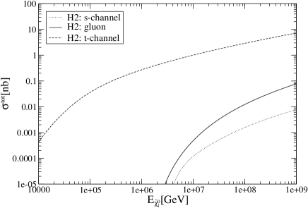
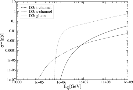
Figure 11: The total cross section for $\tilde{\chi}_{1}^{0}+g\rightarrow\tilde{t}\bar{t},\ \bar{\tilde{t}}t$ (solid curves) in comparison with the $s-$ (dotted) and $t-$channel (dashed curves) contributions.

The added cross section of $\tilde{\chi}_{1}^{0}g\rightarrow\tilde{t}\bar{t}$ and $\tilde{\chi}_{1}^{0}g\rightarrow\bar{\tilde{t}}t$ for a higgsino– and bino–like neutralino are displayed in the left and right frames of Fig. 11, respectively; we used $m_{\tilde{t}_{1}}=1.2$ TeV, $m_{\tilde{t}_{2}}=1.7$ TeV, $\theta_{\tilde{t}}=0.03$ in scenario H2, and $m_{\tilde{t}_{1}}=0.76$ TeV, $m_{\tilde{t}_{2}}=0.91$ TeV, $\theta_{\tilde{t}}=1.4$ in scenario D3. We see that in both cases $t+\tilde{t}$ production only make sub–dominant contributions to the total cross section, although in scenario H2 it dominates the total squark production cross section; the reason is that higgsinos couple proportional to the mass of the quark, as shown by the second term of each of Eqs.(A). Note also that the average energy loss in $t+\tilde{t}$ production will be even larger than in $s-$channel reactions involving light quarks. These processes can therefore be important for higgsino–like LSP if $2m_{\tilde{t}_{1}}\raisebox{-3.69899pt}{~{}\shortstack{$<$ \\ [-0.07cm] $\sim$}}~{}|\mu|<|M_{1}|,\,|M_{2}|$ (which does not happen in mSUGRA [15]), or in scenarios with bino–like LSP if $\tilde{t}_{1}$ is much lighter than first or second generation squarks (which can happen even in mSUGRA, if $|A_{0}|$ is large).

References

- [1] Fly’s Eye Collab., D. Bird et al., Ap. J. 441, 144 (1995).
- [2] AGASA Collab., H. Hayashida et al., Astropart. Phys. 10, 303 (1999).
- [3] For reviews, see P. Bhattacharjee and G. Sigl, Phys. Rep. 327, 109 (2000), astro–ph/9811011; S. Sarkar, hep–ph/0202013; M. Kachelriess, Comptes Rendus Physique 5, 441 (2004), hep–ph/0406174.
- [4] K. Greisen, Phys. Rev. Lett. 16, 748 (1966); G.T. Zatsepin and V.A. Kuzmin, JETP Lett. 4, 78 (1966).
- [5] M. Drees, talk at 9th International Symposium on Particles, Strings and Cosmology (PASCOS 03), Mumbai, India, 3-8 Jan 2003, Pramana 62, 207 (2004), hep–ph/0304030.
- [6] C.T. Hill, Nucl. Phys. B224, 469 (1983); D.N. Schramm and C.T. Hill, Contributed paper to 18th Int. Cosmic Ray Conf., Bangalore, India, August 1983, Cosmic Ray Conf.1983 v.2, 393; C.T. Hill, D.N. Schramm and T.P. Walker, Phys. Rev. D36, 1007 (1987); P. Bhattacharjee, C.T. Hill and D.N. Schramm, Phys. Rev. Lett. 69, 567 (1992).
- [7] V. Berezinsky and A. Vilenkin, Phys. Rev. Lett. 79, 5202 (1997), astro-ph/9704257.
- [8] J. Ellis, J. Lopez and D.V. Nanopoulos, Phys. Lett. B247, 257 (1990); C. Coriano, A.E. Faraggi and M. Plümacher, Nucl. Phys. B614, 233 (2001), hep–ph/0107053; K. Hamaguchi, Y. Nomura and T. Yanagida, Phys. Rev. D58, 103503 (1998), hep–ph/9805346, and D59 063507 (1999), hep–ph/9809426; K. Hamaguchi, K.I. Izawa, Y. Nomura and T. Yanagida, Phys. Rev. D60, 125009 (1999), hep–ph/9903207; K. Hagiwara and Y. Uehara, Phys. Lett. B517, 383 (2001), hep–ph/0106320.
- [9] D.J.H. Chung, E.W. Kolb and A. Riotto, Phys. Rev. D60 (1999) 0603504, hep–ph/9809453; D.J.H. Chung, P. Crotty, E.W. Kolb and A. Riotto, Phys. Rev. D64 043503 (2001), hep–ph/0104100; R. Allahverdi and M. Drees, Phys. Rev. Lett. 89, 091302 (2002), hep–ph/0203118.
- [10] M. Birkel and S. Sarkar, Astropart. Phys. 9, 297 (1998), hep–ph/9804285; V. Berenzinsky and M. Kachelriess, Phys. Lett. B434, 61 (1998), hep–ph/9803500; V. Berezinsky and M. Kachelriess, Phys. Rev. D63, 034007 (2001), hep–ph/0009053; C. Coriano and A. E. Faraggi, Phys. Rev. D65, 075001 (2002), hep–ph/0106326; S. Sarkar and R. Toldra, Nucl. Phys. B621, 495 (2002), hep–ph/0108098; Z. Fodor and S.D. Katz, Phys. Rev. Lett. 86, 3224 (2001), hep–ph/0008204; A. Ibarra and R. Toldra, JHEP 0206, 006 (2002), hep–ph/0202111; V. Berezinsky, M. Kachelriess and S. Ostapchenko, Phys. Rev. Lett. 89, 171802 (2002), hep–ph/0205218; R. Aloisio, V. Berezinsky and M. Kachelriess, Phys. Rev. D69, 094023 (2004), hep–ph/0307279.
- [11] C. Barbot and M. Drees, Phys. Lett. B533,107 (2002), hep–ph/0202072, and Astropart. Phys. 20, 5 (2003), hep–ph/0211406.
- [12] R.A. Vazquez et al., Astropart. Phys. 3, 151 (1995); M. Ave, J.A. Hinton, R.A. Vazquez, A.A. Watson and E. Zas, Phys. Rev. Lett. 85, 2244 (2000), astro–ph/0007386, and Phys. Rev. D65, 063007 (2002), astro–ph/0110613; AGASA collab., K. Shinozaki et al., Astrophys. J. 571, L120 (2002).
- [13] J.R. Ellis, V.E. Mayes and D.V. Nanopoulos, astro–ph/0512303; N. Busca, D. Hooper and E.W. Kolb, astro–ph/0603055.
- [14] C.T. Hill and D.N. Schramm, Phys. Lett. B131, 247 (1983); P. Gondolo, G. Gelmini and S. Sarkar, Nucl. Phys. B392, 111 (1993), hep–ph/9209236; C. Barbot, M. Drees, F. Halzen and D. Hooper, Phys. Lett. B555, 22 (2003), hep–ph/0205230.
- [15] M. Drees, R.M. Godbole and P. Roy, Theory and Phenomenology of Sparticles, World Scientific Publishing Company (2004).
- [16] V. Berezinsky and M. Kachelriess, Phys. Lett. B422, 163 (1998), hep–ph/9709485.
- [17] C. Barbot, M. Drees, F. Halzen and D. Hooper, Phys. Lett. B563, 132 (2003), hep–ph/0207133.
- [18] L. Anchordoqui, H. Goldberg and P. Nath, Phys. Rev. D70, 025014 (2004), hep–ph/0403115.
- [19] A. Datta, D. Fargion and B. Mele, JHEP 0509, 007 (2005), hep–ph/0410176.
- [20] S. Ritz and D. Seckel, Nucl. Phys. B304, 877 (1988); F. Halzen and D. Saltzberg, Phys. Rev. Lett. 81, 4305 (1998), hep-ph/9804354; J. F. Beacom, P. Crotty and E. W. Kolb, Phys. Rev. D66, 021302 (2002), astro-ph/0111482.
- [21] S.I. Dutta, M.H. Reno and I. Sarcevic, Phys. Rev. D61, 053003 (2000), hep–ph/9909393, and Phys. Rev. D62, 123001 (2000), hep-ph/0005310.
- [22] V.A. Naumov and L. Perrone, Astropart. Phys. 10, 239 (1999), hep–ph/9804301.
- [23] E. Reya and J. Rödiger, Phys. Rev. D72, 053004 (2005), hep–ph/0505218.
- [24] J.F. Gunion and H.E. Haber, Nucl. Phys. B272, 1 (1986).
- [25] B.C. Allanach, Comput. Phys. Commun. 143, 305 (2002), hep–ph/0104145.
- [26] A. Djouadi, M. Drees and J.-L. Kneur, hep–ph/0602001.
- [27] S. Kretzer, H.L. Lai, F. Olness and W.K. Tung, Phys. Rev. D69, 114005 (2004), hep–ph/0307022.
- [28] H. Baer, V. Barger, D. Karatas and X. Tata, Phys. Rev. D36 (1987),
- [29] R. Gandhi, C. Quigg, M.H. Reno and I. Sarcevic, Phys. Rev. D58, 093009 (1998), hep–ph/9807264.
- [30] R. Ghandhi, C. Quigg, M.H. Rheno and I. Sarcevic, Astropart. Phys. 5, 81 (1996), hep–ph/9512364.
- [31] EUSO Collab., Ph. Gorodetzky et al., Nucl. Phys. Proc. Suppl. 151, 401 (2006), astro–ph/0502187.
- [32] F.W. Stecker et al., Nucl. Phys. Proc. Suppl. 136C, 433 (2004), astro–ph/0408162.