Abstract

Filon-Simpson quadrature rules are derived for integrals of the type
                 $\int_{a}^{b}dx\,f(x)\>\sin(xy)/(xy)$           and           $\int_{a}^{b}dx\,f(x)\>4\sin^{2}(xy/2)/(xy)^{2}$
which are needed in applications of the worldline variational approach to Quantum Field Theory. These new integration rules reduce to the standard Simpson rule for $y=0$ and are exact for $y\to\infty$ when $a=0$ and $f(0)\neq 0$. The subleading term in the asymptotic expansion is also reproduced more and more precisely when the number of integration points is increased. Tests show that the numerical results are indeed stable over a wide range of $y$-values whereas usual Gauss-Legendre quadrature rules are more precise at low $y$ but fail completely for large values of $y$. The associated Filon-Simpson weights are given in terms of sine and cosine integrals and have to be evaluated for each value of $y$. A Fortran program to calculate them in a fast and accurate manner is available. A detailed omparison is made with the double exponential method for oscillatory integrals due to Ooura and Mori.

1 Introduction

Many problems in theoretical and computational physics require numerical integration over rapidly oscillating functions which usually is considered a difficult, if not hopeless problem. However, as Iserles has pointed out in Ref. [1] this must not be the case: If the quadrature rule for an integral of the type

$$\int_{0}^{h}dx\>f(x)\,e^{ixy}\>\simeq\>\sum_{i=0}^{N}w_{i}f(x_{i})$$ (1.1)

includes the endpoints $x_{0}=0,x_{N}=h$ then the error can be reduced to ${\cal O}\left(h^{N+2}/y^{2}\right)$ for $y\to\infty$. In Iserles’ words: As long as right methods are used, quadrature of highly-oscillatory integrals is very accurate and affordable ! This result rules out the usual quadrature schemes of Gaussian type but is realized in the classic Filon integration rules [2] which are covered in many standard books (see, e.g. chapter 2.10 in Ref. [3] or Eqs. 25.4.47 - 25.4.57 in Ref. [4]).

The present note is not concerned with the numerical evaluation of the Fourier integral (1.1) which is well treated in numerous works but with oscillatory integrals whose integrand has a removable singularity at the origin, viz.

$$I_{1}[f](a,b,y)\>:=\>\int_{a}^{b}dx\>f(x)\,\frac{\sin(xy)}{xy}$$ (1.2)

and

$$I_{2}[f](a,b,y)\>:=\>\int_{a}^{b}dx\>f(x)\>4\,\frac{\sin^{2}(xy/2)}{x^{2}y^{2}}\>.$$ (1.3)

The corresponding weight functions have been normalized in such a way that they become unity for vanishing external (frequency) parameter $y$. In Eq. (1.3) one could rescale $y\to 2y$ to obtain a simpler oscillating weight function. However, due to $\sin^{2}t=(1-\cos(2t)/2$ it would oscillate with twice the frequency and therefore we prefer to define $I_{2}$ in the above form. This is also how it appears in the applications we will discuss below. Note the relation

$$I_{1}[f](a,b,y)\>=\>\frac{1}{2y}\frac{\partial}{\partial y}\,\left[\,y^{2}I_{2}[f](a,b,y)\,\right]\>.$$ (1.4)

As frequently is the case the necessity to evaluate numerically integrals of the type (1.2, 1.3) arose from a concrete theoretical problem. Here it was the polaron problem in solid state physics [5] and its extension, the worldline variational approach to relativistic Quantum Field Theory [6, 7, 8, 9, 10, 11, 12]. With a general quadratic trial action the Feynman-Jensen variational principle gives rise to a pair of non-linear variational equations for the “profile function” $A(E)$ and the “pseudotime” $\mu^{2}(\sigma)$. For example, when calculating the self-energy of a single scalar particle in $d$ space-time dimensions these equations are of the form

$$A(E) = 1+\frac{8}{d}\,\frac{1}{E^{2}}\int_{0}^{\infty}d\sigma\>\frac{\delta V}{\delta\mu^{2}(\sigma)}\>\sin^{2}\left(\frac{E\sigma}{2}\right)$$ (1.5)

$$\mu^{2}(\sigma) = \frac{4}{\pi}\int_{0}^{\infty}dE\>\frac{1}{A(E)}\,\frac{\sin^{2}(E\sigma/2)}{E^{2}}\>.$$ (1.6)

Here $\>V[\mu^{2}]\>$ is the interaction term averaged over the trial action. It is a functional of the pseudotime and specific for the field theory under consideration. For small proper times $\sigma$ its functional derivative (or “force”) has the behaviour

$$\frac{\delta V}{\delta\mu^{2}(\sigma)}\>\stackrel{{\scriptstyle\sigma\to 0}}{{\longrightarrow}}\>\frac{{\rm constant}}{\sigma^{d-2+r}}$$ (1.7)

where $r=0$ for super-renormalizable theories and $r=1$ for renormalizable ones like Quantum Electro-Dynamics (QED). Thus for the 3-dimensional polaron problem and for super-renormalizable theories in 4 dimensions no divergences are encountered in the variational equations but QED₄ needs extra regularization, e.g. a cut-off at high momentum/small proper time. In any case, at least the relation (1.6) between profile function and pseudotime requires evaluation of integrals of the type (1.3) and frequently the proper-time derivative

$$\frac{d\mu^{2}(\sigma)}{d\sigma}\>=\>\frac{2}{\pi}\,\int_{0}^{\infty}dE\>\frac{1}{A(E)}\,\frac{\sin(E\sigma)}{E}\>,$$ (1.8)

i.e. integrals of the type (1.2) are also needed.

Of course, Eqs. (1.5, 1.6, 1.8) involve infinite upper limits but the large-$E,\sigma$ limit of profile function and pseudotime may be obtained analytically so that we can restrict ourselves to finite integration limits and add the analytically calculated asymptotic contribution to the numerical result. Numerical evaluation of Fourier integrals with infinite upper limits is much more demanding; one strategy (employed in the adaptive NAG routine D01ASF [13] based on Ref. [14]) requires a delicate extrapolation procedure and thus seems to be not suitable for a numerical solution of the variational equations.

Previously we have solved these equations on a grid of Gaussian points by iteration (for details see refs. [7]) using Gauss-Legendre quadrature for the oscillatory integrals. Although sufficient for many purposes problems of numerical stability became more serious, in particular in QED₄ when the momentum cut-off was increased too much. It should be mentioned that in the 1-body sector the profile function can be eliminated alltogether giving rise to a non-linear integro-differential equation for the pseudotime only which shows a striking resemblance to the classical Abraham-Lorentz-Dirac equation [15]. This eliminates the need for numerical evaluation of oscillatory integrals but requires solution of non-linear delay-type equations. In addition, at present this is restricted to the 1-body case and for the 2-body, bound-state case we had to apply the previous scheme based on (several) profile functions and pseudotimes [12, 16]. Hence there is a definite need to have a reliable, fast and stable method for evaluating integrals of the type (1.2, 1.3).

In the following sections these integration rules are derived “naively” (that is without mathematical rigor and error estimates) and tested for simple cases. Of course, there is a rich mathematical literature on quadrature rules for various or general oscillatory integrals (for recent developments see, e.g., refs. [17, 18, 19]) but here the emphasis is more on the practical implementation and availability. In addition, the behaviour for large values of the parameter $y$ will be investigated in some detail.

2 Filon-Simpson quadrature

The strategy for deriving a stable quadrature formula for oscillating integrals of the type

$$\int_{a}^{b}dx\>f(x)\>O_{j}(xy)\simeq\sum_{i=0}^{N}w_{i}^{(j)}f\left(x_{i}^{(j)}\right)\>,\>\>O_{j}(xy)\>=\>\left\{\begin{array}[]{r@{\quad:\quad}l}\frac{\sin(xy)}{xy}&j=1\\ \frac{4\sin^{2}(xy/2)}{x^{2}y^{2}}&j=2\end{array}\right.$$ (2.1)

is well known [1]: choose $N$ points $x_{i}^{(j)}$ in the interval $[a,b]$, two of them identical with the endpoints and require that the integral over $x^{k}O_{j}(xy)$ is exact. This gives a system of equations for the integration points $x_{i}^{(j)}$ and weights $w_{i}^{(j)}$.

Here, for simplicity, we choose equidistant, $j$-independent points

$$x_{i}^{(j)}\>\equiv\>x_{i}\>=\>a+ih\>,\>\>i=0\ldots N\>,\>\>h\>=\>\frac{b-a}{N}$$ (2.2)

and $N=2$. In other words: this will be a generalization of Simpson’s time-honoured rule, to which it should reduce for $O_{j}(xy=0)=1$. It is for this reason that we may call it Filon-Simpson quadrature. The integration points being fixed there are three monomials which can be integrated exactly giving rise to three equations for the weights

$$\sum_{i=0}^{2}w_{i}^{(j)}x_{i}^{k}\>=\>\int_{a}^{b=a+2h}dx\>x^{k}\>O_{j}(xy)\>:=\>J_{k}^{(j)}\>,\>\>\>k=0,1,2\>\>.$$ (2.3)

It is easy to solve this linear system of equations with the result

$$w_{0}^{(j)} = \frac{1}{2h^{2}}\,\left[\,x_{1}\,x_{2}\,J_{0}^{(j)}-\left(x_{1}+x_{2}\right)\,J_{1}^{(j)}+J_{2}^{(j)}\,\right]$$ (2.4)

$$w_{1}^{(j)} = \frac{1}{2h^{2}}\,\left[\,-2x_{0}\,x_{2}\,J_{0}^{(j)}+4\,x_{1}\,J_{1}^{(j)}-2J_{2}^{(j)}\,\right]$$ (2.5)

$$w_{2}^{(j)} = \frac{1}{2h^{2}}\,\left[\,x_{0}\,x_{1}\,J_{0}^{(j)}-\left(x_{0}+x_{1}\right)\,J_{1}^{(j)}+J_{2}^{(j)}\,\right]\>.$$ (2.6)

Note that the weights depend on the lower and upper integration limit as well as on the external parameter $y$:

$$w_{i}^{(j)}\>\equiv\>w_{i}^{(j)}(a,b,y)\>,\>\>h\>=\>\frac{b-a}{2}\>.$$ (2.7)

The relation (1.4) translates into

$$J_{k}^{(1)}\>=\>\frac{1}{2y}\frac{\partial}{\partial y}\,y^{2}\,J_{k}^{(2)}\>,\>\>k=0,1,2\>\Rightarrow\>w_{i}^{(1)}\>=\>\frac{1}{2y}\frac{\partial}{\partial y}\,y^{2}\,w_{i}^{(2)}\>,\>\>i=0,1,2$$ (2.8)

and the integrals may be written as

$$J_{k}^{(j)}\>=\>\frac{1}{y^{k+1}}\,\left[\,F_{k}^{(j)}(by)-F_{k}^{(j)}(ay)\,\right]$$ (2.9)

with

$$F_{k}^{(j)}(z)\>=\>\int_{0}^{z}dt\>t^{k}\,O_{j}(t)\>.$$ (2.10)

From the explicit form of the weight functions $O_{k}^{(j)}$ one finds

$$F_{0}^{(1)}(z) = {\rm Si}(z)\>,\>\>F_{1}^{(1)}(z)\>=\>1-\cos z\>,\>\>F_{2}^{(1)}(z)\>=\>\sin z-z\cos z$$ (2.11)

$$F_{0}^{(2)}(z) = 2\,\left[\,{\rm Si}(z)-\frac{1-\cos z}{z}\,\right]\>,\>\>F_{1}^{(2)}(z)\>=\>2\,\left[\,\gamma+\ln z-{\rm Ci}(z)\,\right]\>,$$ (2.12)

$$F_{2}^{(2)}(z) = 2\,\left[\,z-\sin z\,\right]\>.$$ (2.13)

Here $\gamma=0.5772156640\ldots$ is Euler’s constant and ${\rm Si}(z),{\rm Ci}(z)$ the sine and cosine integral, respectively, as defined in chapter 5 of Ref. [4]. Note that the integrals $J_{k}^{(j)}$ are odd under exchange $a\leftrightarrow b$ as may be seen from their definition or from Eq. (2.9). Therefore we find

$$w_{i}^{(j)}(b,a,y)\>=\>-\,w_{2-i}^{(j)}(a,b,y)\>\>,\>\>i\>=\>0,1,2$$ (2.14)

which reflects the basic property of the integrals $I_{j}[f]$ when their limits are exchanged.

As a check we now consider the limit $y\to 0$. It is easily seen that the integrals $J_{k}^{(j)}$ and therefore the weights $w_{i}^{(j)}$ are well-behaved in that limit because we have

$$F_{k}^{(j)}(z)\>=\>z^{k+1}\,\sum_{n=0}^{\infty}\,(-1)^{n}\frac{j}{(2n+j)!}\,\frac{z^{2n}}{2n+k+1}\>.$$ (2.15)

Therefore

$$J_{k}^{(j)}\>\stackrel{{\scriptstyle y\to 0}}{{\longrightarrow}}\>\frac{1}{k+1}\,\left[b^{k+1}-a^{k+1}\right]+{\cal O}\left(y^{2}\right)\>.$$ (2.16)

Eqs. (2.6 - 2.4) and $b=a+2h$ then immediately give the standard Simpson weights

$$w_{0}^{(j)},\,w_{1}^{(j)},\,w_{2}^{(j)}\>\stackrel{{\scriptstyle y\to 0}}{{\longrightarrow}}\>\frac{h}{3},\,\frac{4h}{3},\,\frac{h}{3}+{\cal O}\left(y^{2}\right)\>,$$ (2.17)

independent of the lower limit $a$ and the type $j$ of the integral as it should be.

More interesting is the limit $y\to\infty$ for the case $a=0$. First, the exact asymptotic behaviour of the integrals $I_{j}$ is easily obtained by substituting $t=xy$ :

$$I_{j}[f](a=0,b,y)\>=\>\frac{1}{y}\,\int_{0}^{by}dt\>f\left(\frac{t}{y}\right)\,O_{j}(t)\>\>\stackrel{{\scriptstyle y\to\infty}}{{\longrightarrow}}\>\>\frac{f(0)}{y}\,\int_{0}^{\infty}dt\>O_{j}(t)\>=\>\frac{f(0)}{y}\,\frac{j\pi}{2}\>,\>\>j=1,2\>.$$ (2.18)

The asymptotic limit of the weights is found by employing the expansions [4]

$${\rm Si}(z)\>\stackrel{{\scriptstyle z\to\infty}}{{\longrightarrow}}\>\frac{\pi}{2}-\frac{\cos z}{z}-\frac{\sin z}{z^{2}}+\ldots\>,\hskip 28.45274pt{\rm Ci}(z)\>\stackrel{{\scriptstyle z\to\infty}}{{\longrightarrow}}\>\frac{\sin z}{z}+\ldots$$ (2.19)

which leads to

$$J_{0}^{(j)} \>\stackrel{{\scriptstyle y\to\infty}}{{\longrightarrow}}\> \frac{j}{y}\,\frac{\pi}{2}+{\cal O}\left(\frac{1,\cos by}{y^{2}}\right)$$

$$J_{1}^{(j)} \>\stackrel{{\scriptstyle y\to\infty}}{{\longrightarrow}}\> \frac{2j-2}{y^{2}}\ln by+{\cal O}\left(\frac{1,\cos by}{y^{2}}\right)$$ (2.20)

$$J_{2}^{(j)} \>\stackrel{{\scriptstyle y\to\infty}}{{\longrightarrow}}\> {\cal O}\left(\frac{1,\cos by}{y^{2}}\right)\>.$$

Therefore $J_{0}^{(j)}$ provides the leading asymptotic contribution and from Eqs. (2.4 - 2.6) we see that for $x_{0}=a=0$ only $w_{0}^{(j)}$ is affected by it:

$$w_{0}^{(j)} \>\stackrel{{\scriptstyle y\to\infty}}{{\longrightarrow}}\> \frac{j}{y}\,\frac{\pi}{2}+{\cal O}\left(\frac{(2j-2)\ln by,1,\cos by}{y^{2}}\right)$$ (2.21)

$$w_{1}^{(j)},\,w_{2}^{(j)} \>\stackrel{{\scriptstyle y\to\infty}}{{\longrightarrow}}\> {\cal O}\left(\frac{(2j-2)\ln by,1,\cos by}{y^{2}}\right)\>.$$ (2.22)

Hence Filon-Simpson quadrature gives in that limit

$$\sum_{i=0}^{2}w_{i}^{(j)}f(ih)\>\>\stackrel{{\scriptstyle y\to\infty}}{{\longrightarrow}}\>\>w_{0}^{(j)}f(0)\>=\>\frac{j}{y}\frac{\pi}{2}\,f(0)$$ (2.23)

in perfect agreement with the leading asymptotic result (2.18) !

Of course, the story is different if the function $f(x)$ vanishes at $x=0$: then the next-to-leading terms of the asymptotic expansion come into play. These are studied in more detail in Appendix A1 and A2 where it is shown that for small enough increment $h$ the subleading terms are also reproduced approximately. For example, derivatives are replaced by finite differences as is expected from a quadrature rule which is based on values and not derivatives [19] of the function to be integrated.

3 Extended Filon-Simpson rule

We would like to decrease the error of the quadrature rule in a systematic way without messing up the construction. For equidistant integration points this is, of course, very easy to achieve by dividing the integration interval in $N/2$ sub-intervals, $N$ being even, and applying the integration rule in each sub-interval. We then obtain the ‘extended’ (or ’composite’) Filon-Simpson quadrature rule

$$\boxed{\int_{a}^{b}dx\>f(x)\,O_{j}(xy)\>\simeq\>\sum_{i=0}^{N}W_{i}^{(j)}\,f(a+ih)\>}\>,\>\>h\>=\>\frac{b-a}{N}\>,\>\>N\>{\rm even}$$ (3.1)

where (using the explicit nomenclature of Eq. (2.7))

$$W_{0}^{(j)} = w_{0}^{(j)}(a,a+2h,y)$$ (3.2)

$$W_{i}^{(j)} = w_{1}^{(j)}\left(a+(i-1)h,a+(i+1)h,y\right)\hskip 28.45274pti=1,3\ldots(N-1)$$ (3.3)

$$W_{i}^{(j)} = w_{2}^{(j)}\left(a+(i-2)h,a+ih,y\right)+w_{0}^{(j)}\left(a+ih,a+(i+2)h,y\right)\hskip 14.22636pti=2,4\ldots(N-2)$$ (3.4)

$$W_{N}^{(j)} = w_{2}^{(j)}\left(a+(N-2)h,a+Nh,y\right)\>.$$ (3.5)

Because of the complicated dependence of the weights $w_{i}^{(j)}$ on the lower and upper integration limit it is not possible to simplify the above expressions for $y\neq 0$. Only for $y=0$ we obtain the weights for the extended Simpson rule

$$W_{i}^{(j)}\>\stackrel{{\scriptstyle y\to 0}}{{\longrightarrow}}\>\frac{h}{3}\left\{\begin{array}[]{r@{\quad:\quad}l}1&i=0,N\\ 4&i=1,3\ldots(N-1)\\ 2&i=2,4\ldots(N-2)\>.\end{array}\right.$$ (3.6)

The asymptotic limit $y\to\infty$ for $a=0$ is also unchanged from the the previous section: this is because only in the first interval from $a=0$ up to $2h$ the leading term $\pi/2$ from the asymptotic expansion (2.19) of the sine integral survives whereas in the next and all other intervals it is cancelled due to difference which has to be taken in Eq. (2.9). Thus in the extended Filon-Simpson quadrature rule asymptotic high oscillations are also treated correctly in leading order. Appendix A3 shows that this also holds for the subleading term if the increment $h$ is made small enough, i.e. if the number $N$ of integration points is increased. This is a remarkable feature since logarithmic terms show up in the next-to-leading order of the asymptotic expansion of $I_{2}[f]$ (see Appendix A1). However, Eq. (2.12) shows that by construction such terms are also present in the Filon-Simpson rule for $I_{2}[f]$.

4 Numerical tests

Here we report test evaluations of the integrals

$$I_{j}\left[f_{l}=x^{l}e^{-x}\right]\Bigl{(}a=0,b=\infty,y\Bigr{)}\>=\>\int_{0}^{\infty}dx\>x^{l}\,e^{-x}\,O_{j}(xy)$$ (4.1)

for $l=0,1$ with the Filon-Simpson and other quadrature rules. The oscillatory weight functions $O_{j}(xy)$ have been defined in Eq. (2.1). The exact values of the test integrals are (see e.g. p. 234 – 235 in Ref. [20])

$$I_{1}[f_{0}] = \frac{\arctan(y)}{y}\>,\>\>I_{1}[f_{1}]\>=\>\frac{1}{1+y^{2}}$$ (4.2)

$$I_{2}[f_{0}] = \frac{1}{y^{2}}\left[2y\arctan(y)-\ln\left(1+y^{2}\right)\right]\>,\>\>I_{2}[f_{1}]\>=\>\frac{1}{y^{2}}\ln\left(1+y^{2}\right)$$ (4.3)

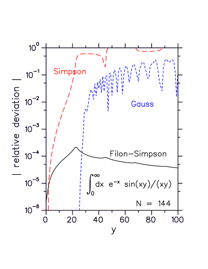
Figure 1: Absolute value of the relative deviation between numerical and exact result for the oscillatory integral $I_{1}[f_{0}]$ as a function of the frequency parameter $y$. The numerical result was obtained with different quadrature rules by numerical integration up to $b=20$ and adding the asymptotic contribution (4.6). The integrand is the function $f_{0}(x)=e^{-x}$ times the oscillatory weight function $O_{1}(xy)=\sin(xy)/(xy)$ and $144$ integration points have been used.

and fulfill the relation (1.4). As discussed in the Introduction our strategy is to perform the numerical integration up to $x=b$ and to add the asymptotic contribution

$$\Delta_{jl}\>:=\>\int_{b}^{\infty}dx\>x^{l}\,e^{-x}\,O_{j}(xy)\>.$$ (4.4)

Due to the specific form (2.1) of the weight functions $O_{j}$ it can be expressed in terms of the exponential integral [4], viz.

$$\Delta_{1l}\>=\>\frac{b^{l}}{y}\,{\rm Im}\,{\rm E}_{1-l}\left((1-iy)b\right)\>,\>\>\Delta_{2l}\>=\>\frac{2b^{l-1}}{y^{2}}\,{\rm Re}\,\Bigl{[}\,{\rm E}_{2-l}(b)-{\rm E}_{2-l}\left((1-iy)b\right)\,\Bigr{]}\>.$$ (4.5)

The asymptotic expansion of these functions gives

$$\Delta_{1l} \simeq \frac{b^{l-1}}{1+y^{2}}\,e^{-b}\,\left[\,\cos by+\frac{\sin by}{y}+{\cal O}\left(\frac{1}{b}\right)\,\right]$$ (4.6)

$$\Delta_{2l} \simeq 2\frac{b^{l-2}}{1+y^{2}}\,e^{-b}\,\left[\,\frac{1+y^{2}+y\sin by-\cos by}{y^{2}}+{\cal O}\left(\frac{1}{b}\right)\,\right]$$ (4.7)

which is well-behaved even for $y=0$. In all numerical calculations we have chosen

$$b\>=\>20$$ (4.8)

so that in general only a very small fraction ${\cal O}\left(e^{-20}\right)\simeq 5\cdot 10^{-8}$ times powers of $b$ comes from the asymptotic region. We have checked that the next order of the asymptotic expansion does not alter the outcome on the required accuracy level except at $y=0$ where small changes are observed.

The Filon-Simpson weights are given in terms of sine and cosine integrals so that a fast and precise routine for these special functions is mandatory. Fortunately there are many convenient rational approximations available, e.g. in chapter 5 of Ref. [4] or routines from commercial libraries. However, with little extra effort the Chebyshev expansions given in Table 23 of Luke’s comprehensive book [21] provide accurate values for these functions which exceed the double precision arithmetic which we employ. Therefore we have used these expansions in a Fortran subroutine making the whole program for calculating Filon-Simpson weights self-contained and portable .

Fig. 1 shows the relative deviation of the numerically calculated integral $I_{1}[f_{0}]$ plus asymptotic contribution from the exact result (4.2) as a function of the external variable $y$. $144$ integration points have been used for both the Filon-Simpson and Simpson rule and $2\times 72$ points for the Gauss-Legendre quadrature (i.e. subdivision of the whole interval in 2 parts and application of a 72-point Gauss-Legendre rule in each part). In Fig. 2 the number of integration points is increased to $288$ and $4\times 72$ respectively. It is seen that for small $y$ the Gauss-Legendre rule is superior but starts to deteriorate when the number of integration points is insufficient for the rapid oscillations of the integrand.

By increasing the number of integration points the onset of failure can be extended (from $y\simeq 25$ in Fig. 1 to $y\simeq 50$ in Fig. 2) but not avoided . The ordinary Simpson rule is even less capable to deal with such type of integrals. In contrast, the new Filon-Simpson quadrature rule gives stable results for all $y$-values considered and its relative deviation from the exact result is a smooth function of $y$ decreasing for very large $y$. Of course, the calculation of the weights has to be redone for each value of $y$ and is more involved than for the standard, simple integration rules. However, in terms of CPU-time this is still a neglible expense (200 $y$-values in Fig. 2 took about 2.5 seconds on a 600 MHz Alpha workstation).

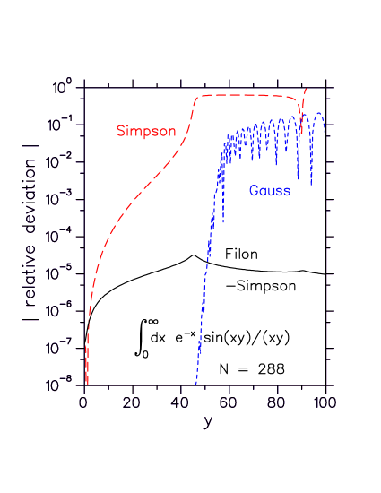
Figure 2: As in Fig. 1 but with $288$ integration points. Note the extended scale for the relative deviations.

Fig. 3 depicts the result for the test function $f_{1}$ which has an additional $x$-power in the integrand so that the relative accuracy which can be achieved with a fixed number of integration points is worse than in the previous case. In addition now $f_{1}(0)=0$ so that the leading asymptotic term vanishes but Appendix A3 demonstrates that the subleading term is also reproduced for sufficiently large number of integration points. Therefore Filon-Simpson integration still does far better than ordinary Simpson or Gauss-Legendre rules.

The corresponding results for the integral $I_{2}[f_{l}]$, i.e. with the weight function $4\sin^{2}(xy/2)/(xy)^{2}$ are shown in Figs. 4 and 5 and confirm the experience gained with $I_{1}$.

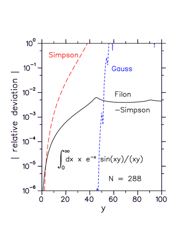
Figure 3: Same as in Fig. 1 but for the test function $f_{1}(x)=xe^{-x}$ and $288$ integration points.

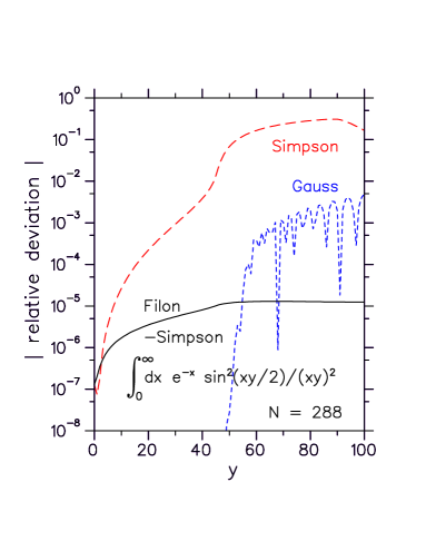
Figure 4: Same as in Fig. 2 but with the oscillatory weight function $O_{2}(xy)$ and the asymptotic contribution (4.7).

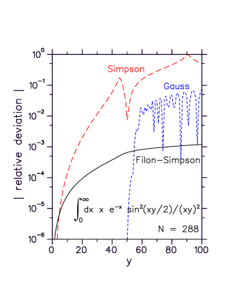
Figure 5: Same as in Fig. 3 but with the oscillatory weight function $O_{2}(xy)$ and the asymptotic contribution (4.7).

Finally, we have investigated whether it is advantagous to use the relation

$$I_{2}[f](a,b,y)\>=\>\frac{2}{y^{2}}\,\int_{0}^{y}dy^{\prime}\>y^{\prime}\,I_{1}[f](a,b,y^{\prime})$$ (4.9)

which is obtained from Eq. (1.4) by integration (the integration constant is zero since the integrals $I_{j}$ are finite at $y=0$). Here one doesn’t have to integrate over an oscillating function and the asymptotic limit (2.18) is also correctly obtained. In the worldline application this would amount to first evaluate $d\mu^{2}(\sigma)/d\sigma$ from Eq. (1.8) and then integrate it step by step via a trapezoidal or Simpson rule to obtain $\mu^{2}(\sigma)$.

Fig. 6 shows the comparison with the direct Filon-Simpson integration. While a lot of accuracy is lost at small $y$ with this procedure reasonable accuracy can be achieved at larger values of the frequency parameter $y$. However, high accuracy requires a precise and smooth input $I_{1}[f](a,b,y^{\prime})$ together with a fine mesh of $y^{\prime}$-values. Considering how fast and easy the Filon-Simpson weights can be generated this procedure does not offer real advantages and is not recommended.

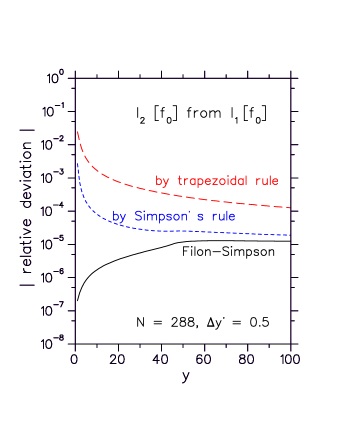
Figure 6: Absolute value of the relative deviation between numerical and exact result if the relation (4.9) is used to obtain the integral $I_{2}[f_{0}]$ from $I_{1}[f_{0}]$. The latter was calculated by the Filon-Simpson routine with 288 points $+$ asymptotic contribution as function of $y^{\prime}$ in steps of $\Delta y^{\prime}=0.5$ and then numerically integrated over $y^{\prime}$ using either the trapezoidal rule or Simpson’s rule. For comparison the result from the direct evaluation of $I_{2}[f_{0}]$ by the Filon-Simpson rule with 288 integration points $+$ asymptotic contribution (as in Fig. 4) is also shown.

5 Comparison with the Double Exponential Method

The double exponential method of Takashi and Mori [22] is based on the Euler-Maclaurin summation formula  (or equivalently the trapezoidal rule)

$$\int_{a}^{b}dxf(x)\>=\>h\sum_{k=0}^{N}f(a+kh)-\frac{h}{2}\left[f(a)+f(b)\right]-\sum_{k=1}^{m-1}\frac{h^{2k}B_{2k}}{(2k)!}\left[f^{(2k-1)}(b)-f^{(2k-1)}(a)\right]+R_{m}$$ (5.1)

with

$$R_{m}\>=\>-\frac{h^{2m+1}B_{2m}}{(2m)!}\,\sum_{k=0}^{N-1}f^{(2m)}(a+kh+\theta h)\>,\qquad 0<\theta<1$$ (5.2)

and the following observation: When $f(x)$ and all its derivatives vanish at the endpoints $a$ and $b$ then the error of the trapezoidal approximation to the integral is given by $R_{m}$ only and for an analytic function ($m\to\infty$) it goes to zero more rapidly than any power of $h$. Indeed if $f(x)$ is analytic in a strip $\>|{\rm Im}\,t|<d\>$ it has be shown [23] that

$$R_{\infty}\>\sim\>e^{-{\rm const}\,d/h}\quad{\rm and}\quad\sim\>e^{-{\rm const^{\prime}}\,N/\log N}\>.$$ (5.3)

This property can be achieved by a special transformation $x=g(t)$ so that

$$\int_{a}^{b}dx\>f(x) = \int_{-\infty}^{+\infty}dt\>g^{\prime}(t)\,f(g(t))$$ (5.4)

$$= h\sum_{k=-\infty}^{+\infty}w_{k}\,f(x_{k})+R(h)\quad{\rm with}\hskip 5.69046ptx_{k}=g(kh)\hskip 5.69046pt{\rm and}\hskip 5.69046ptw_{k}=g^{\prime}(kh)\>.$$

In the second line the trapezoidal rule for the infinite integral is used. The transformation proposed by Takashi and Mori is

$$x\>=\>\frac{b+a}{2}+\frac{b-a}{2}\tanh\left[\,\lambda\,\sinh t\,\right]\>,\hskip 28.45274ptt\in[-\infty,+\infty]\>,\>\>\>\lambda>0$$ (5.5)

from which the alternative name ”tanh-sinh integration rule” is derived (a short introduction is provided by Ref. [24], an overview is given in Ref. [25].) The infinite sum in Eq. (5.4) may be truncated without problems since for $|k|\to\infty$ one has rapid, “double exponential” convergence

$$w_{k}\>\longrightarrow\>\lambda\,(b-a)\,\exp\left(\>-\lambda\,e^{|k|\,h}\>\right)\>.$$ (5.6)

Ooura and Mori [26] (OM) have extended this scheme to oscillatory integrals. Here we describe the method for our integrals

$$I_{j}\>=\>\int_{0}^{\infty}dx\>f(x)\,O_{j}(xy)\quad{\rm with}\quad O_{j}(xy)\>=\>\left(\,\frac{\sin(xy/j)}{xy/j}\,\right)^{j}\>,\quad j=1,2$$ (5.7)

in which $f(x)$ is a non-oscillatory function. Making the variable transformation

$$x\>=\>C_{j}\,g(t)\>,\quad C_{j}>0,\quad t\in[-\infty,+\infty]$$ (5.8)

gives the integral

$$I_{j}\>=\>\int_{-\infty}^{+\infty}dt\>C_{j}\,g^{\prime}(t)\,f\left(C_{j}g(t)\right)\>O_{j}\left(\,C_{j}yg(y)\,\right)\>\simeq\>C_{j}h\sum_{k=-\infty}^{+\infty}g^{\prime}(kh)\,f\left(C_{j}g(kh)\right)\,O_{j}\left(C_{j}yg(kh)\right)$$ (5.9)

and its trapezoidal approximation as usual. However, this time one requires

$$g(-\infty) = 0\>,\quad g^{\prime}(-\infty)\>=\>0$$ (5.10)

$$g(t) \sim t\qquad{\rm for}\qquad t\to+\infty\>.$$ (5.11)

Then one has at large positive $k$

$$f\left(C_{j}g(kh)\right)\,O_{j}\left(C_{j}yg(kh)\right)\>\sim\>f\left(C_{j}kh\right)\,O_{j}\left(C_{j}ykh\right)\>=\>f\left(C_{j}kh\right)\,\left(\,\frac{\sin\left(C_{j}ykh/j\right)}{C_{j}ykh/j}\,\right)^{j}\>.$$ (5.12)

If one chooses the free constant as

$$C_{j}\>=\>\frac{j\pi}{hy}\>,$$ (5.13)

i. e. such that at large $k$ the zeroes of the oscillating function $O_{j}$ are always taken, then

$$\sin\left(C_{j}ykh/j\right)\>=\>\sin(k\pi)\>=\>0\>.$$ (5.14)

This means that one can truncate the summation in Eq. (5.9) at some moderate positive $k$ . For large negative $k$ the summation is restricted due to constraints in Eq. (5.10). Ooura and Mori have given a function $g(t)$ which satisfies all these requirements, viz.

$$\boxed{g_{\rm OM}(t)\>=\>\frac{t}{1-\exp(-2\lambda\sinh t)}\>}\quad,\quad\lambda>0\>,\quad g_{\rm OM}(0)\>=\>\frac{1}{2\lambda}\>,\quad g^{\prime}_{\rm OM}(0)\>=\>\frac{1}{2}\>.$$ (5.15)

Indeed for $t\to\pm\infty$ function values and derivatives approach the required limits in the typical double exponential way

$$g_{\rm OM}(t) \to t\,\Theta(t)+|t|\exp\left[-\lambda e^{|t|}\right]$$

$$g^{\prime}_{\rm OM}(t) \to \Theta(t)-\lambda te^{|t|}\,\exp\left[-\lambda e^{|t|}\right]\>.$$ (5.16)

Thus

$$\boxed{I_{j}[f]\>=\>\int_{0}^{\infty}dx\>f(x)\,O_{j}(xy)\>\simeq\>\frac{j\pi}{y}\,\sum_{k=-k_{\rm max}}^{+k_{\rm max}}\,w_{k}\,f\left(\,\frac{j\xi_{k}}{y}\,\right)\>\left(\,\frac{\sin\xi_{k}}{\xi_{k}}\,\right)^{j}}$$ (5.17)

with

$$w_{k}\>=\>g^{\prime}_{\rm OM}(kh)\quad,\qquad\xi_{k}\>=\>\frac{\pi}{h}\,g_{\rm OM}(kh)\>.$$ (5.18)

Note that the weights $w_{k}$ and the abscissas $\xi_{k}$ in Eq. (5.18) are independent of $j$ and $y$ .

There are several advantages of the OM method:

a)

There is no need to cut off the infinite integral at a large value $\>x=b\>$ and add the asymptotic contribution. Of course, there is an implicit cut-off for the summation over $\>|k|<k_{\rm max}\>$ which turns into a choice of the stepsize for the trapezoidal integration. From the asymptotic behavior in Eq. (5.16) we choose it as

$$\exp\left[\,-\lambda\,\exp\left(\,k_{\rm max}h\,\right)\,\right]\>\leq\>\epsilon\quad\Longrightarrow\>\>h\>=\>\frac{1}{k_{\rm max}}\ln\left[\,-\frac{1}{\lambda}\ln(\epsilon)\,\right]$$ (5.19)

so that the weights are sufficiently small at $\>k=-k_{\rm max}\>$ and sufficiently close to $1$ at $\>k=+k_{\rm max}\>$. Typically we take

$$\epsilon\>=\>10^{-12}\quad,\quad\>\lambda\>=\>1/2\>.$$ (5.20)

b)

Abscissas and weights for different values of the external parameter $\>y\>$ are easily calculated by a simple division or by an overall rescaling (see Eqs. (5.18) and (5.17)).

c)

Only elementary functions are needed.

d)

Automatic programs in Fortran and C are already available and can be downloaded from
                  http://www.kurims.kyoto-u.ac.jp/ ooura/intde.html.
In particular, for the present case the routine
                  intdeo : integrator of f(x) over (a,infinity),  f(x) is oscillatory function
can be used.

$y\quad$	$\>I_{1}[f_{0}]\>$	$\>I_{1}[f_{1}]\>$	$\>I_{2}[f_{0}]\>$	$\>I_{2}[f_{1}]\>$
$0.01$	$-3.04\,(-08)$	$||<\,(-15)$	$-6.07\,(-08)$	$-1.68\,(-13)$
$0.02$	$-1.52\,(-08)$	$||<\,(-15)$	$-3.04\,(-08)$	$-2.81\,(-14)$
$0.05$	$-6.08\,(-09)$	$||<\,(-15)$	$-1.21\,(-08)$	$\>\>\>1.83\,(-14)$
$0.1\>\>$	$-3.04\,(-08)$	$||<\,(-15)$	$-6.08\,(-09)$	$||<\,(-15)$
$0.2\>\>$	$-1.54\,(-09)$	$||<\,(-15)$	$-3.06\,(-09)$	$-2.04\,(-15)$
$0.5\>\>$	$-6.54\,(-10)$	$||<\,(-15)$	$-1.26\,(-09)$	$||<\,(-15)$
$1\quad$	$-3.86\,(-09)$	$||<\,(-15)$	$-6.92\,(-10)$	$||<\,(-15)$
$2\quad$	$-2.74\,(-10)$	$||<\,(-15)$	$-4.31\,(-10)$	$||<\,(-15)$
$5\quad$	$-2.21\,(-10)$	$||<\,(-15)$	$-2.90\,(-10)$	$||<\,(-15)$
$10\quad\,$	$-2.06\,(-10)$	$||<\,(-15)$	$-2.45\,(-10)$	$||<\,(-15)$
$20\quad\,$	$-2.00\,(-10)$	$||<\,(-15)$	$-2.21\,(-10)$	$\>\>\>4.28\,(-15)$
$50\quad\,$	$-1.96\,(-10)$	$4.19\,(-14)$	$-3.38\,(-10)$	$-4.82\,(-08)$
$100\quad\>$	$-1.94\,(-10)$	$4.79\,(-12)$	$-2.92\,(-07)$	$-6.90\,(-05)$
$200\quad\>$	$-1.94\,(-10)$	$4.68\,(-11)$	${\bf-1.10\,(-05)}$	${\bf-2.40\,(-03)}$
$500\quad\>$	$-1.93\,(-10)$	$1.83\,(-10)$	${\bf-1.17\,(-04)}$	${\bf-2.54\,(-02)}$
$1,000\quad\>$	$-1.93\,(-10)$	$2.88\,(-10)$	${\bf-2.93\,(-04)}$	${\bf-6.57\,(-02)}$
$2,000\quad\>$	$-1.93\,(-10)$	$3.62\,(-10)$	${\bf-4.97\,(-04)}$	${\bf-1.19\,(-01)}$
$5,000\quad\>$	$-1.93\,(-10)$	$4.14\,(-10)$	${\bf-7.29\,(-04)}$	${\bf-1.95\,(-01)}$
$10,000\quad\>$	$-1.93\,(-10)$	$4.34\,(-10)$	${\bf-8.52\,(-04)}$	${\bf-2.49\,(-01)}$
$20,000\quad\>$	$-1.93\,(-10)$	$4.44\,(-10)$	${\bf-9.34\,(-04)}$	${\bf-2.99\,(-01)}$
$50,000\quad\>$	$-1.93\,(-10)$	$4.49\,(-10)$	${\bf-9.98\,(-04)}$	${\bf-3.57\,(-01)}$
$100,000\quad\>\>$	$-1.93\,(-10)$	$4.51\,(-10)$	${\bf-1.02\,(-03)}$	${\bf-3.95\,(-01)}$

Table 1: Relative error for the different oscillatory integrals obtained with the double exponential method of Ooura & Mori using $\>2k_{\rm max}+1=289\>$ function calls. Throughout the table the abbreviation $3.0\,(-08)$ for $3.0\cdot 10^{-8}$ etc. is employed and the parameters of Eq. (5.20) are used. $||<\,(-15)$ indicates that the absolute value of the relative deviation is smaller than $10^{-15}$ and thus subject to rounding errors in double precision arithmetic. Errors larger in magnitude than those obtained by the Filon-Simpson method with $N=288$ are printed in boldface.

A disadvantage is that $\>y=0\>$ must be treated separately and does not reduce automatically to the standard tanh-sinh method of Takashi and Mori for the integral over the non-oscillatory function $\>f(x)\>$. Also – in contrast to the Filon-Simpson method – the correct asymptotic behaviour of the oscillatory integrals for $\>y\to\infty\>$ – is not built in. This shows up in the numerical results for the relative error

$$\epsilon_{\rm rel}\>:=\>\frac{I_{j}^{\rm OM}[f_{l}]-I_{j}^{\rm exact}[f_{l}]}{I_{j}^{\rm exact}[f_{l}]}\quad,\quad j=1,2\quad l=0,1$$ (5.21)

for small and large $y$ collected in Table 1: whereas the Ooura-Mori method yields superior results when applied to the test functions with the oscillatory weight $\>O_{1}=\sin(xy)/(xy)\>$ it starts to deteriorate for the oscillatory weight $\>O_{2}=4\sin^{2}(xy/2)/(xy)^{2}\>$ when $y$ becomes large so that finally the Filon-Simpson method takes the lead. Of course, this can be remedied by enlarging $\>k_{\rm max}\>$ and/or taking a smaller stepsize $h$ as Table 2 demonstrates but this makes the method much less efficient in terms of function calls.

Changing the value of the parameter $\lambda$ in the OM method is of no help either: for example, the relative error of $I_{2}^{\rm OM}[f_{1}]$ for $\>y=100,000\>$ (last item in the last line of Table 1) becomes $-0.431$ when $\lambda=3$ is taken as in Ref. [26] .

$y\qquad$	$I_{2}[f_{0}]\>,\qquad|\epsilon_{\rm rel}|<10^{-6}$		$I_{2}[f_{1}]\>,\qquad|\epsilon_{\rm rel}|<10^{-3}$
	OM	FS	OM	FS
$100\quad\>$	$249$	$632$	$189$	$308$
$200\quad\>$	$295$	$674$	${\bf 353}$	$350$
$500\quad\>$	${\bf 907}$	$594$	${\bf 817}$	$394$
$1,000\quad\>$	${\bf 1,565}$	$498$	${\bf 1,553}$	$418$
$2,000\quad\>$	${\bf 2,673}$	$400$	${\bf 2,965}$	$438$
$5,000\quad\>$	${\bf 5,315}$	$288$	${\bf 7,010}$	$458$
$10,000\quad\>$	${\bf 8,770}$	$220$	${\bf 13,490}$	$474$
$20,000\quad\>$	${\bf 14,230}$	$166$	${\bf 26,010}$	$484$
$50,000\quad\>$	${\bf 26,000}$	$112$	${\bf 62,200}$	$496$
$100,000\quad\>\,$	${\bf 39,740}$	$\>82$	${\bf 120,500}\>$	$504$

Table 2: Number of function calls required for obtaining a magnitude of the relative error less than $10^{-6}$ for $\>I_{2}[f_{0}]\>$ and $10^{-3}$ for $\>I_{2}[f_{1}]\>$, respectively, with the Ooura-Mori (OM) and the Filon-Simpson (FS) method for oscillatory integrals. As in Table 1 the parameters are those of Eq. (5.20) and cases where the OM method is inferior to the FS method are printed in boldface.

How can one understand the results of the OM method for our test integrals at large $y$ ?
This is straightforward for functions $f_{0}(x)$ which do not vanish at the origin (in our test example the function $f_{0}(x)=e^{-x}$ ) because

$$I_{j}^{\rm OM}[f_{0}]\>=\>\frac{j\pi}{y}\,\sum_{k=-k_{\rm max}}^{+k_{\rm max}}\,w_{k}\,f_{0}\left(\,\frac{j\xi_{k}}{y}\,\right)\>\left(\,\frac{\sin\xi_{k}}{\xi_{k}}\,\right)^{j}\>\stackrel{{\scriptstyle y\to\infty}}{{\longrightarrow}}\>\,f_{0}(0)\,\frac{j\pi}{y}\,\sum_{k=-k_{\rm max}}^{+k_{\rm max}}\,w_{k}\left(\,\frac{\sin\xi_{k}}{\xi_{k}}\,\right)^{j}$$ (5.22)

whereas the exact asymptotic value from Eqs. (A.2) and (A.5) is

$$I_{j}^{\rm exact}[f_{0}]\>\stackrel{{\scriptstyle y\to\infty}}{{\longrightarrow}}\>\frac{j\pi}{2y}\,f_{0}(0)\>.$$ (5.23)

Therefore

$$\frac{I_{j}^{\rm OM}[f_{0}]-I_{j}^{\rm exact}[f_{0}]}{I_{j}^{\rm exact}[f_{0}]}\>\stackrel{{\scriptstyle y\to\infty}}{{\longrightarrow}}\>2\sum_{k=-k_{\rm max}}^{+k_{\rm max}}\,w_{k}\,\left(\,\frac{\sin\xi_{k}}{\xi_{k}}\,\right)^{j}-1\>=:\>\delta_{j}^{(0)}$$ (5.24)

where the ”defects” $\delta_{j}^{(0)}$ are universal, i.e. do neither depend on $y$ nor on $f_{0}(0)$ but only on the step-size $h$ and the parameter $\lambda$ (when $k_{\rm max}$ is large enough), see Eq. (5.18). For the results presented in Table 1 these constants have the value

$$\delta_{1}^{(0)}\>=\>-1.926\cdot 10^{-10}\qquad,\qquad\delta_{2}^{(0)}\>=\>-1.059\cdot 10^{-3}$$ (5.25)

That the relative error of $\>\>I_{j}^{\rm OM}[f_{0}]\>,\>\>j=1,2\>$ approaches these constants is clearly seen in the results displayed in Table 1. It is due to the well-known fact that in the large-$y$ limit the constant function $f_{0}(0)$ is not integrated exactly in the double-exponential scheme. Neither are low-order polynomials and therefore we have for functions $f_{1}(x)$ where $f_{1}(0)=0,\>f_{1}^{\prime}(0)\neq 0$

$$I_{j}^{\rm OM}[f_{1}]\>\stackrel{{\scriptstyle y\to\infty}}{{\longrightarrow}}\>f^{\prime}_{1}(0)\,\frac{j^{2}\pi}{y^{2}}\,\sum_{k=-k_{\rm max}}^{+k_{\rm max}}\,w_{k}\,\xi_{k}\,\left(\,\frac{\sin\xi_{k}}{\xi_{k}}\,\right)^{j}\>.$$ (5.26)

Utilizing Eq. (A.2) with the upper limit $b\to\infty$ we thus find that for integrals with the oscillating factor $O_{1}$ the relative error of the OM method still approaches a constant defect

$$\frac{I_{1}^{\rm OM}[f_{1}]-I_{1}^{\rm exact}[f_{1}]}{I_{1}^{\rm exact}[f_{1}]}\>\stackrel{{\scriptstyle y\to\infty}}{{\longrightarrow}}\>\pi\sum_{k=-k_{\rm max}}^{+k_{\rm max}}\,w_{k}\,\sin\xi_{k}-1\>=:\>\delta_{1}^{(1)}\>.$$ (5.27)

For the parameters used in Table 1 we find

$$\delta_{1}^{(1)}\>=\>4.548\cdot 10^{-10}$$ (5.28)

which agrees well with the results of Table 1 at high $y$.

The situation is different for integrals with the oscillating factor $O_{2}$ and vanishing function value at $x=0$ (in our test example the function $f_{1}(x)=x\,e^{-x}$ ): Eq. (A.5) then shows a logarithmic enhancement of the exact integral at asymptotic large values of $y$

$$I_{2}[f_{1}]\>\stackrel{{\scriptstyle y\to\infty}}{{\longrightarrow}}\>\frac{2}{y^{2}}\left[\,f_{1}^{\prime}(0)\ln y+C(\infty)\,\right]\>.$$ (5.29)

In contrast the OM approximation in Eq (5.26) cannot develop a logarithmic dependence for finite $k_{\rm max}$. Thus

$$\frac{I_{2}^{\rm OM}[f_{1}]-I_{1}^{\rm exact}[f_{1}]}{I_{1}^{\rm exact}[f_{1}]} \>\stackrel{{\scriptstyle y\to\infty}}{{\longrightarrow}}\> \frac{2\pi}{\ln y+C(\infty)/f^{\prime}(0)}\sum_{k=-k_{\rm max}}^{+k_{\rm max}}\,w_{k}\,\frac{\sin^{2}\xi_{k}}{\xi_{k}}-1$$ (5.30)

$$\>=:\> \delta_{2}^{(1)}/\ln y-1+{\cal O}\left(\,\frac{1}{\ln^{2}y}\,\right)\>.$$

For the parameters of Table 1 we find

$$\delta_{2}^{(1)}\>=\>6.9735$$ (5.31)

and thus from Eq. (5.30) the predictions $\>I_{2}[f1](y=100,000)=-0.3943\>$ and $\>I_{2}[f1](y=50,000)=-0.3555\>$ which are in good agreement with the last two entries of Table 1. Since the logarithmic enhancement of the exact integral always overwhelms the power-like behaviour of the OM approximation the relative deviation therefore will approach the value $-1$ asymptotically.

Obviously this breakdown of the OM method is due to the fact that the weight function $\>O_{2}\>$ is always positive or zero, i.e. does not really oscillate. This then gives rise to logarithmic terms in the exact integrals (see Eq. (4.3)). Note that the Filon-Simpson method has built in these logarithmic terms as can be seen from Eqs. (2.12), (2.20) and therefore copes much better with the limit $y\to\infty$. This is clearly demonstrated in Table 2.

6 Summary

Relatively simple and straightforward quadrature rules of Filon-Simpson form have been presented which are applicable for numerical integration of oscillatory integrals of the type (1.2, 1.3). They employ equidistant integration points (including the endpoints) and weights which have to be calculated anew for each value of the frequency parameter $y$. The choice of equidistant points allows easy construction of extended Filon-Simpson quadrature rules so that the accuracy of the result can be simply assessed by increasing the number of subdivisions. Inevitably the Filon-Simpson weights are more involved than the ones of standard quadrature rules as they are given in terms of sine and cosine integrals and elementary functions. However, the price for an accurate evaluation of these weights is modest and worthwhile as the Filon-Simpson quadrature rules not only reduce to the ordinary Simpson rule for $y=0$ but also give the leading and subleading terms for $y\to\infty$ provided smooth functions are integrated and the spacing of integration points is fine enough. Although a rigorous error estimate has yet to be given, numerical tests have shown that in this regime they do far better than standard quadrature rules. A detailed numerical comparison is made with the double-exponential method proposed by Ooura and Mori: whereas this method gives superior results for Fourier-sine integrals it requires much more function calls than the Filon-Simpson method when applied to $\sin^{2}(xy)$-type integrands with large values of the frequency parameter $y$.

Given its built-in properties for small and large $y$ the Filon-Simpson method is thus an attractive option for all applications where these types of oscillating integrals have to be evaluated.

Acknowledgement: I would like to thank Prof. A. Iserles for a very kind and helpful correspondence.
Habent sua fata libelli: The first version of this paper was sent to J. Comput. Phys. in 2006 where one referee found it “well written and a nice contribution”, whereas the second one didn’t see “sufficient meat” and urged me to write a totally different (“worthwhile”) paper following his ideas. Although the editor, Prof. Lang, tried to find other solutions this was unacceptable for me. In the end the paper lay dormant until I learned about the ingenious method of Ooura and Mori. This happened when I was waiting at a printer, glancing at some of the printouts and rekindled my interest in efficient computation of oscillatory integrals. I am indebted to the unknown colleague who printed out Ref. [26] just in the right moment…

Appendix

A1 Exact asymptotic behaviour of the integrals

Here we derive the asymptotic expansion of the oscillatory integrals beyond the leading order which was only considered in the main text. We assume that the function $f(x)$ is analytic at $x=0$ and that the upper limit $b$ is finite.

We start with the integral $I_{1}$ whose asymptotic expansion is easy to obtain by a subtraction followed by an integration by parts so that an additional inverse power of $y$ is generated:

$$I_{1}[f](a=0,b,y) = \int_{0}^{b}dx\>f(0)\,\frac{\sin xy}{xy}+\frac{1}{y}\int_{0}^{b}dx\>\frac{f(x)-f(0)}{x}\,\sin xy\>=\>\frac{f(0)}{y}F_{0}^{(1)}(by)$$ (A.1)

$$+\frac{1}{y}\left[-\frac{f(x)-f(0)}{x}\frac{\cos xy}{y}\,\Biggr{|}_{0}^{b}+\frac{1}{y}\int_{0}^{b}dx\,\left(\frac{f(x)-f(0)}{x}\right)^{\prime}\cos xy\,\right].$$

Repeating the process in the remaining integral it is seen that it is of higher order. By using the explicit expression for $F_{0}^{(1)}(by)$ given in Eq. (2.11) together with the asymptotic expansion (2.19) we thus obtain

$$I_{1}[f](a=0,b,y)\>\>\stackrel{{\scriptstyle y\to\infty}}{{\longrightarrow}}\>\>\frac{\pi f(0)}{2y}+\frac{1}{y^{2}}\,\left[f^{\prime}(0)-f(b)\frac{\cos yb}{b}\right]+{\cal O}\left(\frac{\sin by}{y^{3}}\right)\>.$$ (A.2)

Similarly we obtain for the integral $I_{2}[f](a=0,b,y)$ after two subtractions

$$I_{2}[f](a=0,b,y)\>=\>\frac{f(0)}{y}F_{0}^{(2)}(by)+\frac{f^{\prime}(0)}{y^{2}}F_{1}^{(2)}(by)+\frac{2}{y^{2}}\int_{0}^{b}dx\>g(x)\left(1-\cos xy\right)$$ (A.3)

where $g(x)=(f(x)-f(0)-xf^{\prime}(0))/x^{2}$ is regular at $x=0$. Therefore we may apply the procedure of repeated integration by parts to obtain for the last term

$$\frac{2}{y^{2}}\int_{0}^{b}dx\>g(x)\left(1-\cos xy\right)\>=\>\frac{2}{y^{2}}\int_{0}^{b}dx\>g(x)-\frac{2}{y^{3}}\,g(x)\sin xy\Biggr{|}_{0}^{b}+\ldots\>.$$ (A.4)

Finally by employing the explicit expressions for $F_{j}^{(2)}(by)$ given in Eq. (2.13) together with the asymptotic expansions (2.19) we obtain

$$I_{2}[f](a=0,b,y)\>\>\stackrel{{\scriptstyle y\to\infty}}{{\longrightarrow}}\>\>\frac{\pi f(0)}{y}+\frac{2}{y^{2}}\left[\,f^{\prime}(0)\,\ln y+C(b)\,\right]-\frac{2f(b)\sin by}{b^{2}y^{3}}+\ldots\>.$$ (A.5)

Formally the last term in Eq. (A.5) is of next-to-next-to-leading order but it is needed to verify the relation (1.4) to next-to-leading order. Note also the appearance of logarithmic terms in the asymptotic expansion of $I_{2}$ ; the constant $C(b)$ in Eq. (A.5) is given by

$$C(b)\>=\>\left(\,\gamma+\ln b\,\right)\,f^{\prime}(0)-\frac{f(0)}{b}+\int_{0}^{b}dx\>\frac{f(x)-f(0)-xf^{\prime}(0)}{x^{2}}\>.$$ (A.6)

Three integration by parts in the last integral bring it into the form

$$C(b)\>=\>\gamma f^{\prime}(0)-\frac{f(b)}{b}+f^{\prime}(b)+\left[\,f^{\prime}(b)-bf^{\prime\prime}(b)\,\right]\,\ln b+\int_{0}^{b}dx\>x\ln x\,f^{\prime\prime\prime}(x)$$ (A.7)

which will be needed for comparison with the extended Filon-Simpson rule.

It is clear that nothing prevents the procedure to be extended to arbitrary order but for our purposes this is not needed. One may check the asymptotic expansions (A.2, A.5) by applying them to the functions $f_{l}(x)$ used for the numerical tests: in the limit $b\to\infty$ one obtains full agreement with the first terms of the asymptotic expansion of the exact results (4.2, 4.3).

A2 Asymptotic behaviour of the Filon-Simpson rules

How do the Filon-Simpson quadrature rules behave in the asymptotic limit ? To answer this question we just have to plug the asymptotic expansions of the functions $F_{i}^{(j)}(by)$ into the expressions for the weights. After some algebraic work we obtain

$$\sum_{i=0}^{2}w_{i}^{(1)}\,f_{i}\>=\>\frac{1}{y}\frac{\pi}{2}f_{0}+\frac{1}{y^{2}}\left[\,\stackrel{{\scriptstyle\rightarrow}}{{\delta}}\!\!f_{0}-\frac{f_{2}\cos by}{b}\,\right]+{\cal O}\left(\frac{\sin by}{y^{3}}\right)\>,\hskip 14.22636pta\>=\>0,\>b=2h$$ (A.8)

where $f_{i}\equiv f(ih)$ and

$$\stackrel{{\scriptstyle\rightarrow}}{{\delta}}\!\!f_{0}\>=\>\frac{1}{2h}\,\left[\,-3f(0)+4f(h)-f(2h)\,\right]\>\stackrel{{\scriptstyle h\to 0}}{{\longrightarrow}}\>f^{\prime}(0)-\frac{1}{3}h^{2}f^{\prime\prime\prime}(0)+\ldots\>.$$ (A.9)

Thus one obtains the correct subleading term of the asymptotic expansion except that the derivative of the function at $x=0$ is replaced by its (forward) finite-difference approximation $\stackrel{{\scriptstyle\rightarrow}}{{\delta}}\!\!f_{0}$.

Similarly, one finds that for the integral $I_{2}[f]$ the Filon-Simpson quadrature rule has the asymptotic expansion

$$\sum_{i=0}^{2}w_{i}^{(2)}\,f_{i}\>=\>\frac{1}{y}\pi f_{0}+\frac{2}{y^{2}}\left[\,\stackrel{{\scriptstyle\rightarrow}}{{\delta}}\!\!f_{0}\cdot\ln y+C_{FS}(b)\right]+{\cal O}\left(\frac{\sin by}{y^{3}}\right)\hskip 14.22636pta\>=\>0,\>b=2h$$ (A.10)

where the constant is given by

$$C_{FS}(b)\>=\>\left(\,\gamma+\ln b\,\right)\,\stackrel{{\scriptstyle\rightarrow}}{{\delta}}\!\!f_{0}-\frac{f_{0}}{b}+\frac{b}{2}\,\delta^{2}f_{1}\>.$$ (A.11)

Here

$$\delta^{2}f_{1}\>=\>\frac{1}{h^{2}}\,\left[\,f(0)-2f(h)+f(2h)\,\right]\>\stackrel{{\scriptstyle h\to 0}}{{\longrightarrow}}\>f^{\prime\prime}(0)+hf^{\prime\prime\prime}(0)+\ldots=f^{\prime\prime}(h)+{\cal O}\left(h^{2}\right)$$ (A.12)

is a finite-difference approximation to the second derivative of the function $f(x)$ at $x=0$ (or better at $x=h$). Comparing with the exact next-to-leading term in the asymptotic expansion of $I_{2}[f]$ we see that again finite differences are subsituted for derivatives and that the last integral in Eq. (A.6) is replaced by

$$\int_{0}^{b}dx\>\frac{f(x)-f(0)-xf^{\prime}(0)}{x^{2}}\>\simeq\>\int_{0}^{b}dx\>\left[\,\frac{1}{2}f^{\prime\prime}(0)+\ldots\,\right]\>=\>\frac{b}{2}f^{\prime\prime}(0)+\ldots$$ (A.13)

which is valid for regular functions and increments $b=2h$ which are small enough.

A3 Asymptotic behaviour of the extended Filon-Simpson rules

Let us now investigate how the extended Filon-Simpson rules behave in the limit $y\to\infty$. To do that we need the asymptotic behaviour of the simple rules in intervals with non-zero lower limit. Using the quadrature rules in the form

$$\sum_{i=0}^{2}w_{i}^{(j)}f_{i}\>=\>\left[\,f_{0}-a\stackrel{{\scriptstyle\rightarrow}}{{\delta}}\!\!f_{0}+\frac{a^{2}}{2}\delta^{2}f_{1}\,\right]\,J_{0}^{(j)}+\left[\,\stackrel{{\scriptstyle\rightarrow}}{{\delta}}\!\!f_{0}-a\,\delta^{2}f_{1}\,\right]\,J_{1}^{(j)}+\frac{1}{2}\delta^{2}f_{1}\,J_{2}^{(j)}$$ (A.14)

we obtain for the Filon-Simpson quadrature of $I_{1}[f]$

$$\sum_{i=0}^{2}w_{i}^{(1)}f_{i}\>\>\stackrel{{\scriptstyle y\to\infty}}{{\longrightarrow}}\>\>\frac{1}{y^{2}}\,\left[\,\frac{f_{0}}{a}\cos ay-\frac{f_{2}}{b}\cos by\,\right]\>,\hskip 11.38092pta\neq 0,\>b=a+2h$$ (A.15)

and therefore

$$\sum_{i=0}^{N}w_{i}^{(1)}f_{i} \>\stackrel{{\scriptstyle y\to\infty}}{{\longrightarrow}}\> \frac{\pi f_{0}}{2y}+\frac{1}{y^{2}}\,\left[\,\stackrel{{\scriptstyle\rightarrow}}{{\delta}}\!\!f_{0}-f_{2}\frac{\cos(2hy)}{2h}\,\right]$$ (A.16)

$$\hskip 22.76228pt+\frac{1}{y^{2}}\,\left[\,\frac{f_{2}}{2h}\cos(2hy)-\frac{f_{4}}{4h}\cos 4hy\,\right]+\ldots$$

$$\hskip 2.84544pt\ldots\,+\frac{1}{y^{2}}\,\left[\,\frac{f_{2N-2}}{(2N-2)h}\cos((2N-2)hy)-\frac{f_{N}}{Nh}\cos(2Nh)\,\right]\>.$$

Here the first line gives the contribution from the first interval $[0,2h]$ (see Eq. (A.8)), the second line the one from the second interval $[2h,4h]$ and so on. It is seen that in the $1/y^{2}$-terms the contributions cancel pairwise and only the ones from the first and the last interval survive. Therefore

$$\sum_{i=0}^{N}w_{i}^{(1)}f_{i}\>\>\stackrel{{\scriptstyle y\to\infty}}{{\longrightarrow}}\>\>\frac{\pi f_{0}}{2y}+\frac{1}{y^{2}}\,\left[\,\stackrel{{\scriptstyle\rightarrow}}{{\delta}}\!\!f_{0}-\frac{f_{N}}{Nh}\cos 2Nh\,\right]+\ldots$$ (A.17)

which is again the correct asymptotic result (A.2) except that the derivative of the function at $x=0$ is replaced by the finite difference $\stackrel{{\scriptstyle\rightarrow}}{{\delta}}\!\!f_{0}$.

The subleading asymptotic terms for the Filon-Simpson quadrature of $I_{2}[f]$ are more involved because of the logarithmic terms. From Eq. (A.14) and the asymptotic behaviour of the integrals $J_{k}^{(2)}$ one gets after some algebra

$$\sum_{i=0}^{2}w_{i}^{(2)}f_{i} \>\stackrel{{\scriptstyle y\to\infty}}{{\longrightarrow}}\> \frac{2}{y^{2}}\,\Biggl{[}\,\frac{f_{0}}{a}-\frac{f_{2}}{b}+2h\delta^{2}f_{1}+\left(\stackrel{{\scriptstyle\leftarrow}}{{\delta}}\!\!f_{2}-b\,\delta^{2}f_{1}\right)\,\ln b$$ (A.18)

$$\hskip 99.58464pt-\left(\stackrel{{\scriptstyle\rightarrow}}{{\delta}}\!\!f_{0}-a\,\delta^{2}f_{1}\right)\,\ln a\,\Biggr{]}\>,\hskip 11.38092pta\neq 0,\>b=a+2h\>.$$

Here

$$\stackrel{{\scriptstyle\leftarrow}}{{\delta}}\!\!f_{2}\>=\>\frac{1}{2h}\left[f_{0}-4f_{1}+3f_{2}\right]\>\stackrel{{\scriptstyle h\to 0}}{{\longrightarrow}}\>f_{2}^{\prime}-\frac{h^{2}}{3}f^{\prime\prime\prime}_{2}+\ldots$$ (A.19)

is the backward finite-difference approximation for the derivative of the function $f(x)$ at the point $x_{2}=b=a+2h$. It is obtained from the (forward) form (A.9) by the exchange $a\leftrightarrow b$.

Together with the result (A.10) for the first interval we therefore have

$$\sum_{i=0}^{N}w_{i}^{(2)}f_{i} \>\stackrel{{\scriptstyle y\to\infty}}{{\longrightarrow}}\> \frac{\pi f_{0}}{y}+\frac{2}{y^{2}}\,\Biggl{\{}\,\stackrel{{\scriptstyle\rightarrow}}{{\delta}}\!\!f_{0}\,(\gamma+\ln y)+\frac{f_{2}-f_{0}}{2h}-\frac{f_{N}}{Nh}+h\delta^{2}f_{1}+2h\sum_{i=2}^{N/2}\delta^{2}f_{2i-1}$$ (A.20)

$$+\left(\stackrel{{\scriptstyle\rightarrow}}{{\delta}}\!\!f_{0}-\stackrel{{\scriptstyle\rightarrow}}{{\delta}}\!\!f_{2}+2h\delta^{2}f_{3}\right)\,\ln(2h)+\left(\stackrel{{\scriptstyle\leftarrow}}{{\delta}}\!\!f_{N}-Nh\delta^{2}f_{N-1}\right)\,\ln(Nh)$$

$$+2h\sum_{i=2}^{N/2-1}\left[\,\frac{\stackrel{{\scriptstyle\leftarrow}}{{\delta}}\!\!f_{2i}-\stackrel{{\scriptstyle\rightarrow}}{{\delta}}\!\!f_{2i}}{2h}+2ih\frac{\delta^{2}f_{2i+1}-\delta^{2}f_{2i-1}}{2h}\,\right]\,\ln(2ih)\,\Biggl{\}}\>.$$

At first sight this looks rather complicated unless one recognizes the sums as (extended) trapezoidal rules with stepsize $2h$ for the corresponding integrals (see, e.g. Eq. (25.4.2) in Ref. [4])

$$2h\,\left[\,\frac{g_{0}}{2}+g_{2}+g_{4}+\ldots+g_{N-2}+\frac{g_{N}}{2}\,\right]\>=\>\int_{0}^{Nh}dx\>g(x)+{\cal O}\left(h^{3}\right)\>.$$ (A.21)

Furthermore

$$\frac{f_{2}-f_{0}}{2h}\>\stackrel{{\scriptstyle h\to 0}}{{\longrightarrow}}\>f_{0}^{\prime}\>,\hskip 19.91684pt\stackrel{{\scriptstyle\rightarrow}}{{\delta}}\!\!f_{0}-\stackrel{{\scriptstyle\rightarrow}}{{\delta}}\!\!f_{2}+2h\delta^{2}f_{3}\>=\>{\cal O}\left(h^{2}\right)\>,$$

$$\frac{\stackrel{{\scriptstyle\leftarrow}}{{\delta}}\!\!f_{2i}-\stackrel{{\scriptstyle\rightarrow}}{{\delta}}\!\!f_{2i}}{2h}\>=\>{\cal O}\left(h^{3}\right)\>,\hskip 19.91684pt\frac{\delta^{2}f_{2i+1}-\delta^{2}f_{2i-1}}{2h}\>\stackrel{{\scriptstyle h\to 0}}{{\longrightarrow}}\>f^{\prime\prime\prime}_{2i}\>.$$ (A.22)

Therefore in the limit $h\to 0$ Eq. (A.20) becomes

$$\sum_{i=0}^{N}w_{i}^{(2)}f_{i} \>\stackrel{{\scriptstyle y\to\infty}}{{\longrightarrow}}\> \frac{\pi f_{0}}{y}+\frac{2}{y^{2}}\,\Biggl{\{}\,f^{\prime}(0)\,(\gamma+\ln y)+f^{\prime}(0)-\frac{f(b)}{b}+\int_{0}^{b}dx\>f^{\prime\prime}(x)$$ (A.23)

$$\hskip 22.76228pt+\left[\,f^{\prime}(b)-bf^{\prime\prime}(b)\,\right]\,\ln b\,+\int_{0}^{b}dx\>x\ln x\,f^{\prime\prime\prime}(x)\Biggr{\}}$$

which agrees exactly with the subleading term of Eq. (A.5) and the form (A.7) of the constant $C(b)$.

References

• [1] A. Iserles: On the numerical quadrature of highly-oscillating integrals, I: Fourier transforms, IMA J. Num. Anal. 24 (2004), 365 – 391.
• [2] L. N. G. Filon: On a quadrature formula for trigonometric integrals, Proc. Royal Soc. Edinburgh 49 (1928), 38 – 47.
• [3] P. J. Davis and P. Rabinowitz: Methods of Numerical Integration, Academic Press, New York (1975).
• [4] M. Abramowitz and I. Stegun (eds.): Handbook of Mathematical Functions, Dover (1965).
• [5] R. Rosenfelder and A. W. Schreiber: On the best quadratic approximation in Feynman’s path integral treatment of the polaron, Phys. Lett. A 284 (2001), 63 - 71   [arXiv:cond-mat/0011332] .
• [6] R. Rosenfelder and A. W. Schreiber: Polaron Variational Methods in the Particle Representation of Field Theory: I. General Formalism, Phys. Rev. D 53 (1996), 3337 – 3353   [arXiv:nucl-th/9504002].
• [7] R. Rosenfelder and A. W. Schreiber: Polaron variational methods in the particle representation of field theory: II. Numerical results for the propagator, Phys. Rev. D 53 (1996), 3354 – 3365   [arXiv:nucl-th/9504005].
• [8] A. W. Schreiber, R. Rosenfelder and C. Alexandrou: Variational calculation of relativistic meson-nucleon scattering in zeroth order, Int. J. Mod. Phys. E 5 (1996), 681 – 716   [arXiv:nucl-th/9504023].
• [9] A. W. Schreiber and R. Rosenfelder: First order variational calculation of form factor in a scalar nucleon–meson theory, Nucl. Phys. A 601 (1996), 397 – 424   [arXiv:nucl-th/9510032].
• [10] C. Alexandrou, R. Rosenfelder and A. W. Schreiber: Variational field theoretic approach to relativistic meson-nucleon scattering, Nucl. Phys. A 628 (1998), 427 – 457   [arXiv:nucl-th/9701036];
N. Fettes and R. Rosenfelder: Inclusive and deep inelastic scattering from a dressed structureless nucleon, Few-Body Syst. 24 (1998), 1 – 25.
• [11] R. Rosenfelder and A. W. Schreiber: Improved variational description of the Wick-Cutkosky model with the most general quadratic trial action, Eur. Phys. J. C 25 (2002), 139 – 156   [arXiv:hep-th/0112212].
• [12] K. Barro-Bergflödt, R. Rosenfelder and M. Stingl: Worldline variational approximation: A new approach to the relativistic binding problem, Mod. Phys. Lett. A 20 (2005), 2533 – 2543   [arXiv:hep-ph/0403304]
• [13] Numerical Algorithm Group: The NAG Fortran Library Manual, Mark 21
http://www.nag.co.uk/numeric/fl/manual/html/FLlibrarymanual.asp
• [14] R. Piessens, E. de Doncker-Kapenga, C. Überhuber and D. Kahaner: QUADPACK, A Subroutine Package for Automatic Integration, Springer (1983).
• [15] R. Rosenfelder and A. W. Schreiber: An Abraham-Lorentz-like equation for the electron from the worldline variational approach to QED, Eur. Phys. J. C 37 (2004), 161 – 172   [arXiv:hep-th/0406062].
• [16] K. Barro-Bergflödt, R. Rosenfelder and M. Stingl: Variational worldline approximation for the relativistic two-body bound state in a scalar model, Few-Body Syst. 39 (2006), 193 – 253 [arXiv: hep-ph/0601220].
• [17] A. Iserles and S. P. Nørsett: On quadrature methods for highly oscillatory integrals and their implementation, BIT 44 (2004), 755 – 772.
• [18] A. Iserles: On the numerical quadrature of highly-oscillating integrals, II: Irregular oscillators, IMA J. Num. Anal. 25 (2005), 25 – 44.
• [19] A. Iserles and S. P. Nørsett: Efficient quadrature of highly oscillatory integrals using derivatives, Proc. Roy. Soc. A 461 (2005), 1383 – 1399.
• [20] H. B. Dwight: Tables of Integrals and Other Mathematical Data, MacMillan, New York (1961).
• [21] Y. L. Luke: The Special Functions and Their Approximations, vol. II, Academic Press, New York (1969).
• [22] H. Takahashi and M. Mori: Double exponential formulas for numerical integration, Publ. RIMS, Kyoto Univ. 9 (1974), 721 – 741.
• [23] M. Mori: Developments in the double exponential formulas for numerical integration, Proc. Int. Congr. of Mathematicians, Kyoto, Japan, (1990), p. 1585 – 1594.
• [24] D. H. Bailey, J. M. Borwein, D. Broadhurst and W. Zudilin: Experimental Mathematics and Mathematical Physics, arXiv:1005.0414.
• [25] M. Mori: Discovery of the double exponential transformation and its developments, Publ. RIMS, Kyoto Univ. 41 (2005), 897 –- 935.
• [26] T. Ooura and M. Mori: The double exponential formula for oscillatory functions over the half infinite interval, J. Comp. Appl. Math. 38 (1991), 353 – 360.
• [27] T. Ooura and M. Mori: A robust double exponential formula for Fourier-type integrals, J. Comp. Appl. Math. 112 (1999), 229 – 241.