Color-superconductivity
in the strong-coupling regime of Landau gauge QCD

Abstract

The chirally unbroken and the superconducting 2SC and CFL phases are investigated in the chiral limit within a Dyson-Schwinger approach for the quark propagator in QCD. The hierarchy of Green’s functions is truncated such that at vanishing density known results for the vacuum and at asymptotically high densities the corresponding weak-coupling expressions are recovered. The anomalous dimensions of the gap functions are analytically calculated. Based on the quark propagator the phase structure is studied, and results for the gap functions, occupation numbers, coherence lengths and pressure differences are given and compared with the corresponding expressions in the weak-coupling regime. At moderate chemical potentials the quasiparticle pairing gaps are several times larger than the extrapolated weak-coupling results.

I Introduction

Strongly interacting matter as it existed in the early universe, resides in the interior of compact stellar objects or is produced in heavy-ion collisions is subject to extreme conditions. An understanding of the different phases of such matter in terms of the fundamental degrees of freedom of QCD in the realm of low temperatures and high quark densities is still missing although such knowledge would be of fundamental interest. At sufficiently high density and low temperatures strongly interacting matter is expected to be a color superconductor, which has re-attracted a lot of interest in recent years (for corresponding reviews see reviews ; Rischke:2003mt ). Due to asymptotic freedom, it can be systematically studied at asymptotically large densities in a weak coupling expansion SchafHong . At densities that are relevant for the interior of neutron stars one is in the strongly coupled regime, and such an expansion is lacking. Investigations AlfRapp are usually done within Nambu-Jona–Lasino-type models in mean-field approximation. The main objective of these studies is the identification of possible scenarios for the color-superconducting state. Since the results are rather model dependent on a quantitative level an approach, which is directly based on the QCD degrees of freedom is highly desirable.

Furthermore, although it has been argued on general grounds that quarks become deconfined at high densities, a corresponding detailed picture is missing. This relates to the fact that already at vanishing temperatures and densities many aspects of the confinement mechanisms remain elusive, in spite of recent progress (see e.g. ref. Greensite:2003bk ). Relations between the confining field configurations and the Gribov horizon have been established Greensite:2004mh . Those are in turn related to the infrared behavior of QCD Green’s functions, either in Coulomb gauge Zwanziger:2003de or in Landau gauge vonSmekal:2000pz QCD. In the Coulomb gauge quark confinement results already from an effective one-gluon exchange picture Zwanziger:2002sh ; Nakamura:2005ux and confinement of colored composite states such as ‘diquarks’ can be studied Alkofer:2005ug . A detailed understanding of the infrared part of the Yang-Mills sector is still lacking, however. On the other hand, in the Landau gauge the gluon propagator has been determined quantitatively by different methods with consistent results, see e.g. Silva:2005hb ; Sternbeck:2005tk ; Fischer:2004uk ; Pawlowski:2003hq ; Alkofer:2003jj and references therein. The infrared behavior of the vacuum gluon and ghost propagators, established by these and related studies, have provided the basis for investigations of the quark propagator as well as extensions to finite temperature for the pure Yang-Mills sector Maas . The results underline non-trivial strong coupling of ghosts and gluons even at arbitrary high temperatures.

It seems natural to suitably extend these methods to finite densities especially for the strongly coupled regime, and compare to analytical results obtained in the weak coupling limit. In the present work we proceed in this direction by extending the truncation scheme of the pertinent Dyson-Schwinger equations (DSE) proposed in ref. Fischer:2003rp . We implement momentum- and energy-dependent self energies, which encode information about the non-Fermi liquid behavior of the chirally unbroken phase at large quark densities. This is important for the analysis of superconducting gap functions already in the weakly coupled regime Wang:2001aq . We consider medium effects on the quark-quark interaction in the random-phase approximation similar to the Hard-Dense-Loop (HDL) approximation and thereby recover the corresponding analytical results in the weakly coupled regime. The presented results allow for a quantitative estimate for the validity of the weak coupling results at a given chemical potential. This is the main objective of the present investigation.

This paper is organized as follows: In sect. II the truncated quark Dyson-Schwinger equation at non-vanishing chemical potential is derived. In sect. III the ultraviolet behavior of the gap functions is extracted analytically. In sect. IV we provide expressions for occupation numbers, diquark coherence lengths and the effective action. In sect. V we discuss the relevance and application of Luttinger’s theorem for relativistic matter. In sect. VI we give numerical results for the unbroken phase. In sect. VII results for two superconducting phases (2SC and CFL) are presented, including an estimate of the pressure from the Cornwall-Tomboulis-Jackiw (CJT) action. Sect. VIII closes with some concluding remarks and an outlook.

II QCD Green’s functions

II.1 The quark propagator at non-vanishing chemical potential

For the description of superconducting systems, it is advantageous to work within the Nambu-Gor’kov formalism Gorkov . In the following we will only consider the chiral limit and thus treat all flavors equally. Extending the conventions and notations of refs. Alkofer:2000wg ; Roberts:2000aa , the unrenormalized QCD Lagrangian in Euclidean space at finite quark chemical potential $\mu$ and vanishing quark masses reads

$$S^{(\mu)}\left[\psi,\bar{\psi},A_{\nu}^{a}\right]=S\left[\psi,\bar{\psi},A_{\nu}^{a}\right]+\bar{\psi}\gamma_{4}\mu\psi$$ (4)

$$= \frac{1}{2}\bar{\Psi}\left(\begin{array}[]{cc}-\gamma_{\mu}D_{\mu}+\gamma_{4}\mu&0\\ 0&-\gamma_{\mu}D_{C\mu}-\gamma_{4}\mu\end{array}\right)\Psi$$

$$\hskip 113.81102pt+\frac{1}{4}F^{a}_{\mu\nu}F^{a}_{\mu\nu}\,,$$

where $D_{C\mu}=\partial_{\mu}-igA^{T}_{\mu}$ corresponds to the charge-conjugate of the covariant derivative $D_{\mu}=\partial_{\mu}+igA_{\mu}$. Using the charge-conjugation matrix of Dirac spinors, $C=\gamma_{2}\gamma_{4}$, the $8N_{c}N_{f}$-dimensional bispinors $\Psi(x)$ are defined as

$$\Psi=\left(\begin{array}[]{c}\psi\\ \psi_{C}=C\bar{\psi}^{T}\end{array}\right),\quad \bar{\Psi}=\left(\bar{\psi},\bar{\psi}_{C}=\psi^{T}C\right).$$ (7)

Note that the components of these bispinor field operators are not independent of each other Rischke:2000ra . In the following $N_{c}=3$ and $N_{f}=3$ will be used.

In a covariant gauge, the renormalized quark DSE with appropriate quark-wave-function and quark-gluon-vertex renormalization constants, $Z_{2}$ and $Z_{1F}$, respectively, is then given by

$$\mathcal{S}^{-1}(p) = Z_{2}\mathcal{S}_{0}^{-1}(p)+Z_{1F}\Sigma(p),$$ (8)

where

$$\mathcal{S}_{0}^{-1}(p) = \left(\begin{array}[]{cc}-i\vec{p}\cdot\vec{\gamma}-i(p_{4}+i\mu+gA_{4})\gamma_{4}&0\\ 0&-i\vec{p}\cdot\vec{\gamma}-i(p_{4}-i\mu-gA_{4}^{T})\gamma_{4}\\ \end{array}\right)$$ (11)

is the inverse bare quark propagator in the presence of a static, isotropic and homogeneous time component $A_{4}$ of the gluon field. The quark self energy $\Sigma(p)$ is given by

$$\Sigma(p)=-\int\!\!\frac{d^{4}q}{(2\pi)^{4}}\Gamma_{NG,\mu}^{(0)a}\mathcal{S}(q)\Gamma^{b}_{NG,\nu}(q,p)D^{ab}_{\mu\nu}(q-p).$$ (12)

Here $D_{\mu\nu}^{ab}(k)$ is the gluon propagator, and the bare and full quark-gluon vertex in the Nambu-Gor’kov basis is defined as

$$\Gamma^{(0)a}_{NG\mu}=\frac{ig}{2}\left(\begin{array}[]{cc}\gamma_{\mu}\lambda^{a}&0\\ 0&-\gamma_{\mu}\lambda^{aT}\end{array}\right),$$ (15)

$$\Gamma^{a}_{NG\mu}(q,p)=\frac{ig}{2}\left(\begin{array}[]{cc}\Gamma^{a}_{\mu}(q,p)&\Delta^{a}_{C\mu}(q,p)\\ \Delta^{a}_{\mu}(q,p)&\Gamma^{a}_{C\mu}(q,p)\end{array}\right),$$ (18)

with $\Delta^{a}_{C\mu}(q,p)=-C\Delta^{a}_{\mu}(-p,-q)^{T}C$ and $\Gamma^{a}_{C\mu}(q,p)=-C\Gamma^{a}_{\mu}(-p,-q)^{T}C$. Flavor indices have been suppressed, they will be discussed in detail below.

In a fixed gauge, the expectation value of $A_{4}$ is determined by its DSE, i.e. by its equation of motion. In a covariant gauge this corresponds to a vanishing expectation value of

$$\frac{\delta S^{(\mu)}[\psi,\bar{\psi},A_{\mu}^{a}]}{\delta A_{\mu}^{a}(x)} = -\left(\partial_{\nu}\delta^{ab}+gf^{abc}A^{c}_{\nu}(x)\right)F^{b}_{\nu\mu}(x)$$ (19)

$$-\frac{1}{2}\bar{\Psi}(x)\Gamma^{(0)a}_{NG\mu}\Psi(x)-\frac{1}{\lambda}\partial_{\mu}\partial_{\nu}A_{\nu}^{a}(x)$$

$$-igf^{abc}\partial_{\mu}\bar{c}_{b}(x)c_{c}(x),$$

where $c(x)$ and $\bar{c}(x)$ is the ghost and antighost field, respectively. For a static, isotropic, homogenous, even-parity and $T$-symmetric ground state $|\Omega\rangle$ in a fixed covariant gauge one has

$$\langle\Omega|D_{\nu}^{ab}F_{\nu\mu}^{b}(x)|\Omega\rangle =$$

$$-gf^{abc}\langle\Omega|A^{c}_{\nu}(x)F^{b}_{\nu\mu}(x)|\Omega\rangle = 0$$ (20)

and, since the ghost propagator is real and symmetric,

$$\langle\partial_{\mu}\bar{c}_{b}(x)c_{c}(x)\rangle=0\leavevmode\nobreak\ .$$ (21)

From this one eventually obtains

$$\rho^{a}(x)\propto\frac{1}{2}\mathrm{Tr}_{D,c,f,NG}\left(\mathcal{S}(x)\Gamma^{(0)a}_{NG4}\right)=0\leavevmode\nobreak\ .$$ (22)

Therefore the static gluon fields ensure color neutrality ($\rho^{a}(x)=0$) and can be implicitly determined by this condition Gerhold:2003js ; Dietrich:2003nu ; Buballa:2005bv . For the symmetries stated above, this is equivalent to the exact solution of the equations of motion. For the quantities discussed in the following the neutrality condition only slightly modifies the results, and thus it will be neglected for simplicity.

II.2 Gluon propagator and quark-gluon vertex

The quark propagator can be determined from eq. (8) as a functional of the gluon propagator and the quark-gluon vertex. In the Landau gauge, which will be employed in the following, these Green’s functions have been investigated for the chirally broken phase at zero chemical potential by DSE studies and by lattice calculations, see e.g. Alkofer:2003jj ; Fischer:2002hn ; Sternbeck:2005tk ; Silva:2005hb ; Bowman:2004jm ; Llanes-Estrada:2004jz ; Skullerud:2004gp ; Lin:2005zd . In the Landau gauge, the gluon propagator is parameterized by a single dressing function $Z(k^{2})$,

$$D_{\mu\nu}^{ab}(k^{2}) = \delta_{ab}\left(\delta_{\mu\nu}-\frac{k_{\mu}k_{\nu}}{k^{2}}\right)\frac{Z(k^{2})}{k^{2}}.$$ (23)

The quark-gluon vertex possesses in general twelve linearly independent Dirac tensor structures (see e.g. ref. Alkofer:2000wg ) with the vector-type coupling $\propto\gamma_{\mu}$ being the only one present at tree level. It has been shown that some of the other tensor structures are qualitatively important when studying the quark DSE Fischer:2003rp ; Alkofer:2003jj . For simplicity, in this exploratory study the quark-gluon vertex is assumed to be of the form

$$\Gamma^{a}_{\mu}(p,q) = ig\Gamma((p-q)^{2})\gamma_{\mu}\frac{\lambda^{a}}{2}.$$ (24)

The unknown function $\Gamma(k^{2})$ has been chosen such that the quark propagator is multiplicatively renormalizable and agrees with perturbation theory in the ultraviolet Fischer:2003rp . It can also be determined from quenched lattice results of the quark and gluon propagator Bhagwat:2003vw or finite-volume results for the corresponding DSE’s in combination with lattice data for the quark propagator Fischer:2005nf . Beyond the vector-type coupling contained in (24) at least the term proportional to $p_{\mu}+q_{\mu}$ is of qualitative significance Fischer:2003rp ; Alkofer:2003jj . In the chiral limit such a scalar-type term is, however, only non-vanishing in the chirally broken phase because such a contribution violates chiral symmetry. As we are interested here in superconducting phases this scalar contribution will not be present, at least, in the chiral limit. Therefore, the use of the approximation (24) is certainly sufficient for an exploratory study.

In the following only the product

$$\alpha_{s}(k^{2}) = \frac{Z_{1F}}{Z_{2}^{2}}\frac{g^{2}}{4\pi}Z(k^{2})\Gamma(k^{2}),$$ (25)

will enter the quark propagator DSE. Here $Z_{1F}$ is the quark-gluon coupling and $Z_{2}$ the quark-wave-function renormalization constant, respectively. We will refer to $\alpha_{s}(k^{2})$ as the effective strong running coupling because, especially in the framework of DSEs, it is a possible non-perturbative extension of the coupling into the infrared.

It is, of course, expected that the gluon propagator and the quark-gluon vertex undergo changes when a non-vanishing chemical potential is introduced. Note that in superconducting phases anomalous vertices, the $\Delta^{a}_{\mu}$ in eq. (18), are induced. These are neglected in the study reported in this paper. Thus, taking into account the matrix structure implied by the Nambu-Gor’kov formalism and the approximation (24) we will use

$$\Gamma^{a}_{NG\mu}(p,q) = \Gamma((p-q)^{2})\Gamma^{(0)a}_{NG\mu},$$ (26)

with $\Gamma(k^{2})$ taken from quenched vacuum studies.

Since we are primarily interested in chirally unbroken phases at non-vanishing chemical potential, it is important to incorporate medium effects like damping and screening by particle-hole excitations. In this paper we add the in-medium polarization tensor with ’bare’ quark propagators to the inverse gluon propagator. This is not self-consistent and needs to be investigated in further studies. Nevertheless, the resulting quark DSE turns out to be a generalization of the HDL approximation, with the important difference that the infrared behavior of the gluon propagator and quark-gluon vertex is nontrivial. Furthermore, even in the superconducting phases, the assumption of bare quark propagators will a posteriori turn out to be much better suited than employing the vacuum quark propagator, i.e. the one reflecting dynamical chiral symmetry breaking.

The renormalized medium polarization tensor is generically given by

$$\Pi_{\phantom{{\rm med}\,}\mu\nu}^{{\rm med}\,ab}(p)=\frac{1}{2}Z_{1F}\int\!\!\frac{d^{4}q}{(2\pi)^{4}}\mathrm{Tr}_{D,c,f,NG}\left(\left[\Gamma^{(0)a}_{NG\mu}\mathcal{S}(q)\Gamma_{NG\nu}^{b}(q,p-q)\mathcal{S}(p-q)\right]-\left[\ldots\right]_{\mu=0}\right)\leavevmode\nobreak\ .$$ (27)

For the first part we employ the approximation of vanishing quark self-energies and the vertex (26). Then this expression can be straightforwardly reduced to

$$\Pi_{\phantom{{\rm med}\,}\mu\nu}^{{\rm med}\,ab}(p) = -\frac{Z_{1F}}{Z_{2}^{2}}\frac{g^{2}N_{f}}{2}\delta^{ab}\Gamma(p^{2})\int\!\!\frac{d^{4}q}{(2\pi)^{4}}\mathrm{Tr}_{D}\left(\left[\gamma_{\mu}S_{0}(q)\gamma_{\nu}S_{0}(p-q)\right]-\left[\ldots\right]_{\mu=0}\right)$$ (28)

$$= -\delta^{ab}\frac{2\pi N_{f}\alpha_{s}(p^{2})}{Z(p^{2})}\int\!\!\frac{d^{4}q}{(2\pi)^{4}}\mathrm{Tr}_{D}\left(\left[\gamma_{\mu}S_{0}(q)\gamma_{\nu}S_{0}(p-q)\right]-\left[\ldots\right]_{\mu=0}\right).$$

With help of projectors transverse and longitudinal to the medium Kapusta:1989tk ,

$$P^{T}_{44}=P^{T}_{i4}=P^{T}_{4i}=0,\quad P^{T}_{ij}=\delta_{ij}-\frac{p_{i}p_{j}}{\vec{p}^{2}},$$

and

$$P^{L}_{\mu\nu}=(\delta_{\mu\nu}-p_{\mu}p_{\nu}/p^{2})-P^{T}_{\mu\nu},$$

respectively, this polarization tensor can be expressed by two functions, $G(|\vec{p}|,p_{4})$ and $F(|\vec{p}|,p_{4})$,

$$Z(p^{2})\Pi_{\mu\nu}^{ab}(p) = G(p)\delta^{ab}P^{T}_{\mu\nu}+F(p)\delta^{ab}P^{L}_{\mu\nu}.$$

The evaluation of this functions is well known perturbatively, and in the present case only the coupling is replaced by the running coupling. For small external momenta, the result is

$$G(|\vec{p}|,p_{4}) = m^{2}(p^{2})\frac{ip_{4}}{|\vec{p}|}\left[\left(1-\left(\frac{ip_{4}}{|\vec{p}|}\right)^{2}\right)\right.$$ (30)

$$\left.Q\left(\frac{ip_{4}}{|\vec{p}|}\right)+\frac{ip_{4}}{|\vec{p}|}\right],$$

$$F(|\vec{p}|,p_{4}) = 2m^{2}(p^{2})\frac{p_{4}^{2}+\vec{p}^{2}}{\vec{p}^{2}}$$ (31)

$$\left[1-\frac{ip_{4}}{|\vec{p}|}Q\left(\frac{ip_{4}}{|\vec{p}|}\right)\right],$$

with $Q(x)=\frac{1}{2}\ln\frac{x+1}{x-1}$ and

$$m^{2}(p^{2})={N_{f}\alpha_{s}(p^{2})\mu^{2}}/{\pi}.$$ (32)

Adding the medium polarization to the inverse gluon propagator leads to

$$D_{\mu\nu}^{ab}(p) \approx \left(D^{vac\,-1}_{\mu\nu}(p^{2})+\Pi_{\phantom{{\rm med}\,}\mu\nu}^{{\rm med}\,ab}(p)\right)^{-1}$$ (33)

$$= \delta^{ab}\Bigl{(}\frac{p^{2}}{p^{2}+G(p)}P^{T}_{\mu\nu}$$

$$+\frac{p^{2}}{p^{2}+F(p)}P^{L}_{\mu\nu}\Bigr{)}\frac{Z(p^{2})}{p^{2}}\leavevmode\nobreak\ .$$

Taking into account this form of the in-medium polarization, Debye screening and Landau damping are included, similar as in the HDL approximation. As it is phrased here, it becomes evident that these phenomena have a non-perturbative origin and require the knowledge of the infrared behavior of Schwinger functions, in particular of $\alpha_{s}(k^{2})$.

II.3 The truncated quark DSE at non-vanishing chemical potential

Summarizing the above considerations we arrive at a truncated, self-consistent DSE for the quark propagator. Treating the components in the Nambu-Gor’kov basis separately we define Rischke:2003mt

$$\mathcal{S}_{0}(p) = \left(\begin{array}[]{cc}S_{0}^{+}(p)&0\\ 0&S_{0}^{-}(p)\end{array}\right),$$ (36)

$$\mathcal{S}(p) = \left(\begin{array}[]{cc}S^{+}(p)&T^{-}(p)\\ T^{+}(p)&S^{-}(p)\end{array}\right),$$ (39)

$$\Sigma(p) = \left(\begin{array}[]{cc}\Sigma^{+}(p)&\Phi^{-}(p)\\ \Phi^{+}(p)&\Sigma^{-}(p)\end{array}\right),$$ (42)

with

$$A^{-}(p) = -C(A^{+}(-p))^{T}C$$ (43)

$${\rm for}\quad A^{\pm} \in \{S_{0}^{\pm},S^{\pm},T^{\pm}\},$$

$\Sigma^{+}(p)+\Sigma^{-}(p)=\gamma_{4}\left(\Sigma^{+}(p)+\Sigma^{-}(p)\right)^{\dagger}\gamma_{4}$ and

$$\Phi^{-}(p)=\gamma_{4}(\Phi^{+}(p))^{\dagger}\gamma_{4}$$ (44)

for a real action. One then obtains Manuel:2000nh

$$T^{\pm} = -Z_{1F}\left(Z_{2}{S^{\mp}_{0}}^{-1}+Z_{1F}\Sigma^{\mp}\right)^{-1}\Phi^{\pm}S^{\pm},$$

$${S^{\pm}}^{-1} = \hphantom{-}Z_{2}{S^{\pm}_{0}}^{-1}+Z_{1F}\Sigma^{\pm}$$

$$- Z_{1F}^{2}\Phi^{\mp}\left(Z_{2}{S^{\mp}_{0}}^{-1}+Z_{1F}\Sigma^{\mp}\right)^{-1}\Phi^{\pm},$$

combined with

$$\Sigma^{+}(p) = \hphantom{-}\frac{Z_{2}^{2}}{Z_{1F}}\pi\int\!\!\frac{d^{4}q}{(2\pi)^{4}}\gamma_{\mu}\lambda_{a}S^{+}(q)\gamma_{\nu}\lambda_{a}$$

$$\left(\frac{\alpha_{s}(k^{2})P^{T}_{\mu\nu}}{k^{2}+G(k)}+\frac{\alpha_{s}(k^{2})P^{L}_{\mu\nu}}{k^{2}+F(k)}\right),$$

$$\Phi^{+}(p) = -\frac{Z_{2}^{2}}{Z_{1F}}\pi\int\!\!\frac{d^{4}q}{(2\pi)^{4}}\gamma_{\mu}\lambda_{a}^{T}T^{+}(q)\gamma_{\nu}\lambda_{a}$$

$$\left(\frac{\alpha_{s}(k^{2})P^{T}_{\mu\nu}}{k^{2}+G(k)}+\frac{\alpha_{s}(k^{2})P^{L}_{\mu\nu}}{k^{2}+F(k)}\right).$$

Note that the running coupling $\alpha_{s}(k^{2})$ also enters via the functions $G(|\vec{k}|,k_{4})$ and $F(|\vec{k}|,k_{4})$. On the other hand, this running coupling is the only input into eqs. (LABEL:gap). In the following we will present results for two different couplings. Both couplings are derived in a MOM regularization scheme. One will be the running coupling determined from the coupled gluon, ghost and quark DSEs Fischer:2003rp , denoted by $\alpha_{I}(k^{2})$ in the following, where

$$\alpha_{I}(k^{2}) = \frac{\alpha_{I}(0)}{\ln\left(e+a_{1}\left(k^{2}/\Lambda_{I}^{2}\right)^{a_{2}}+b_{1}\left(k^{2}/\Lambda_{I}^{2}\right)^{b_{2}}\right)},\quad$$ (47)

with $\alpha_{I}(0)=2.972$, $a_{1}=1.106$, $a_{2}=2.324$, $b_{1}=0.004$, $b_{2}=3.169$ and $\Lambda_{I}=0.714\mathrm{GeV}$. As the quark-gluon vertex used in this study contains a sizeable “scalar” contribution (which is due to dynamical chiral symmetry breaking) the corresponding running coupling together with the approximation (24) underestimates the chiral condensate significantly but should be, as mentioned above, the appropriate choice in chirally restored phases. We consider this coupling as a lower bound. On the other hand, the running coupling extracted from quenched lattice data together with an abelian approximation for the quark-gluon vertex Bhagwat:2003vw serves as an upper bound and will be denoted by $\alpha_{II}(k^{2})$ in the following. As the corresponding parameterization is quite lengthy, we refer to eqs. (8)-(16) of ref. Bhagwat:2003vw for its definition. Both couplings are shown in Fig. 1.

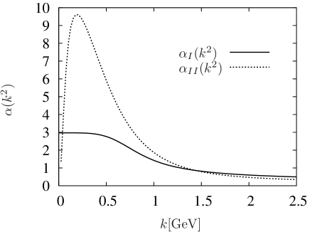
Figure 1: Two versions of the strong running coupling in the numerical solution of the DSE (LABEL:gap). The full line represents the coupling $\alpha_{I}(k^{2})$ extracted from the coupled gluon, ghost and quark DSE’s Fischer:2003rp and the dashed line $\alpha_{II}(k^{2})$ extracted from quenched lattice data together with an abelian approximation for the quark-gluon vertex Bhagwat:2003vw .

In order to obtain a self-consistent solution of the system of equations (LABEL:gap) with (31), (32) and the running coupling as input, we will first consider the color and flavor structure of the quark self energy. We will restrict ourselves to scalar pairing and treat the 2-flavor color-superconducting (2SC) and color-flavor locked (CFL) phases separately. In the chiral limit, the pairing structure can be described by a symmetric matrix $M$ such that the projectors on its eigenspaces $P_{i}$ together with the matrices $M_{i}:=MP_{i}$ form a closed basis under the transformations $P_{i}\to\lambda_{a}P_{i}\lambda_{a}$ and $M_{i}\to\lambda^{T}_{a}M_{i}\lambda_{a}$, respectively. Therefore, we can parameterize the r.h.s. of eqs. (LABEL:gap) by the renormalization point independent, Dirac-algebra valued self energies $\Sigma^{+}_{i}(p)$ and $\phi^{+}_{i}(p)$:

$$\Sigma^{+}(p) = \frac{Z_{2}}{Z_{1F}}\sum_{i}\Sigma^{+}_{i}(p)P_{i},$$ (48)

$$\Phi^{+}(p) = \frac{Z_{2}}{Z_{1F}}\sum_{i}\phi^{+}_{i}(p)M_{i}.$$ (49)

For an even-parity and $T$-symmetric phase those are given by Pisarski:1999av

$$\Sigma^{+}_{i}(p) = -i\vec{p}\!\!/\,\Sigma^{+}_{A,i}(p)-i\omega_{p}\!\!\!\!\!\!/\,\,\,\Sigma^{+}_{C,i}(p)$$ (50)

$$= \gamma_{4}\sum_{e=\pm 1}\Sigma_{e,i}^{+}(p)\Lambda^{e}_{\vec{p}},$$

$$\phi^{+}_{i}(p) = \left(\gamma_{4}\hat{p}\!\!/\,\phi^{+}_{A,i}(p)+\phi^{+}_{C,i}(p)\right)\gamma_{5}$$ (51)

$$= \gamma_{5}\sum_{e=\pm 1}\phi_{e,i}^{+}(p)\Lambda^{e}_{\vec{p}},$$

where we made use of the positive and negative energy projectors $\Lambda^{\pm}_{\vec{p}}=\frac{1}{2}\left(1\pm i\gamma_{4}\hat{p}\!\!/\,\right)$, $\vec{p}\!\!/\,=\vec{p}\cdot\vec{\gamma}$, $\hat{p}=\vec{p}/|\vec{p}|$, $\omega_{p}\!\!\!\!\!\!/\,\,\,=\omega_{p}\gamma_{4}$ and $\omega_{p}=ip_{4}+\mu$.

Introducing positive parameters $\delta_{i}>0$ via the decomposition $M^{\dagger}M=\sum_{i}\delta_{i}P_{i}$ the quark particle-particle propagator can be written as

$$Z_{2}S^{+}(p)=-\gamma_{4}\sum_{i,e=\pm}P_{i}\Lambda^{-e}\frac{\left(-ip_{4}-\mu\right)\left(1+{\Sigma_{C,i}^{+}(p)}^{*}\right)+e|\vec{p}|\left(1+{\Sigma_{A,i}^{+}(p)}^{*}\right)}{|(ip_{4}-\mu)(1+\Sigma_{C,i}^{+}(p))+e|\vec{p}|(1+\Sigma_{A,i}^{+}(p))|^{2}+\delta_{i}|\phi_{e,i}(p)|^{2}},$$

where we have made use of the relations $\Sigma_{F,i}(p)={\Sigma_{F,i}(-p)}^{*}$. The zero of the numerator at $p_{4}=0$ defines the quasiparticle Fermi momenta $p_{F}$, and the zero in the denominator provides the corresponding dispersion relation. To first approximation, the energy gap $\Delta_{i}^{e}$ in the excitation spectrum is therefore given by

$$\Delta_{i}^{e} \simeq \left|\frac{\sqrt{\delta_{i}}\,\phi_{e,i}(p)}{1+\Sigma_{C,i}^{+}(p)}\right|_{|\vec{p}|=p_{F},p_{4}=0}.$$ (53)

III Ultraviolet finiteness of the gap functions

Similar to the ultraviolet analysis of the quark mass function in the chirally broken phase Gusynin:1986fu we determine here the ultraviolet behavior of the gap functions. For large external momenta $p$, such that $\phi^{2}(p)\ll p^{2}$, $\mu^{2}\ll p^{2}$ and $m^{2}\ll p^{2}$, the breaking of Lorentz covariance is negligibly small, and thus the self-energies $\Sigma^{\pm}(p)$ and $\Phi^{\pm}(p)$ are to a very good approximation functions of the four-momentum squared, $p^{2}$, only. Furthermore, in the denominators of the integral kernels the self-energies can be safely neglected. Also the medium modifications of the gluon propagator will then be insignificant, and the gap equations reduce to

$$\sum_{i}\phi^{+}_{C,i}(p)M_{i}\simeq$$

$$\hskip 14.22636pt-3\pi\sum_{i}\int\!\!\frac{d^{4}q}{(2\pi)^{4}}\frac{\phi^{+}_{C,i}(q)}{q^{2}}\frac{\alpha_{s}(k^{2})}{k^{2}}\lambda_{a}^{T}M_{i}\lambda_{a},$$

(54)

$$\sum_{i}\phi^{+}_{A,i}(p)M_{i}\simeq$$

$$\hskip 14.22636pt-\sum_{i}\pi\int\!\!\frac{d^{4}q}{(2\pi)^{4}}\frac{\phi^{+}_{A,i}(q)}{q^{2}}\frac{\alpha_{s}(k^{2})}{k^{2}}\lambda_{a}^{T}M_{i}\lambda_{a}$$

$$\hskip 14.22636pt\times\left(\hat{p}\cdot\hat{q}\left(1-2\frac{k_{4}^{2}+(\hat{q}\cdot\vec{k})^{2}}{k^{2}}\right)\right).$$ (55)

As the running coupling is a slowly varying function for large momenta it is safe to apply the angular approximation $\alpha_{s}(k^{2})\approx\alpha_{s}(p^{2}\,\theta(p^{2}-q^{2})+q^{2}\,\theta(q^{2}-p^{2}))$. The remaining angular integrations can then be done analytically. The gap function $\phi^{+}_{A,i}(p)$ decreases for large $p^{2}$ at least like $1/p^{4}$ times logarithmic corrections, and thus to order $1/p^{2}$, one has $\phi^{+}_{A,i}(p)\approx 0$. The equation for the gap function $\phi^{+}_{C,i}(p)$ then reads

$$\sum_{i}\phi^{+}_{C,i}(p)M_{i} \simeq -\frac{3}{16\pi}\sum_{i}\lambda_{a}^{T}M_{i}\lambda_{a}$$

$$\hskip 8.53581pt\left(\frac{\alpha_{s}(p^{2})}{p^{2}}\int^{p^{2}}\!dq^{2}\,\phi^{+}_{C,i}(q)\right.$$

$$\hskip 8.53581pt\left.+\int_{p^{2}}\!dq^{2}\,\frac{\alpha_{s}(q^{2})\phi^{+}_{C,i}(q)}{q^{2}}\right).$$

The color-antitriplet channel is attractive and for this channel we get $\lambda_{a}^{T}M_{i}\lambda_{a}=-\frac{8}{3}M_{i}$ as compared to $\lambda_{a}\lambda_{a}=\frac{16}{3}=4C_{F}$. The color sextet channel is repulsive. For this one we have $\lambda_{a}^{T}M_{i}\lambda_{a}=\frac{4}{3}M_{i}$. The anomalous dimensions of the gap functions $\gamma_{\phi,i}$, to one-loop order can then be read off from the coefficient in eq. (LABEL:UV). Comparing to the corresponding anomalous dimension of the mass function $\gamma_{m}=12/(33-2N_{f})$, they are given by

$$\gamma_{\phi,\bar{3}}=\phantom{-}\gamma_{m}/2=\phantom{-}6/(33-2N_{f})$$ (57)

and

$$\gamma_{\phi,6}=-\gamma_{m}/4=-3/(33-2N_{f})$$ (58)

in attractive and repulsive channels, respectively. Similar to the chiral quark condensate, see e.g. ref. Roberts:1994dr , one is now able to define a renormalization-group independent diquark condensate. The asymptotic behavior of $\phi^{+}_{C,i}(p)$ is given by the so-called ’regular form’

$$\phi^{+}_{C,i}(p) \propto \frac{1}{p^{2}}\left(\ln\left(\frac{p^{2}}{\Lambda^{2}}\right)\right)^{\gamma_{\phi,i}-1}.$$ (59)

IV Relevant quantities

IV.1 Occupation numbers and diquark correlations

Once the quark propagator is known, one can extract number densities, occupation numbers and the diquark coherence lengths. Within the Euclidean formalism, the number density $\rho$ is calculated as the derivative of the generating functional of the connected Green’s functions with respect to the chemical potential $\mu$. For the homogeneous phases, considered here it is given by

$$\rho = Z_{2}\langle\langle\psi^{\dagger}(\vec{x})\psi(\vec{x})\rangle\rangle$$ (60)

$$= \lim_{x_{4}\rightarrow i0^{+}}\frac{1}{2}\mathrm{Tr}_{D,c,f,NG}\left(Z_{2}\,\gamma_{4}\otimes\mathds{1}_{NG}\mathcal{S}(x_{4},0)\right)$$

$$= \int\!\!\frac{d^{3}\vec{p}}{(2\pi)^{3}}\int\!\frac{dp_{4}}{2\pi}\,\mathrm{Tr}_{D,c,f}\left(Z_{2}\,\gamma_{4}\otimes\mathds{1}_{NG}S^{+}_{q}(p)\right)$$

$$= \sum_{i}\frac{g_{i}}{(2\pi)^{3}}\int d^{3}p\,\,n_{i}(p),$$

where $g_{i}=2\,\mathrm{rank}(P_{i})$ is a degeneracy factor, and the occupation numbers $n_{i}(p)$ read

$$n_{i}(p) = \frac{Z_{2}}{4\pi}\int_{-\infty}^{\infty}\!\!dp_{4}\,\,\mathrm{Tr}_{D}\left(\gamma_{4}S^{+}_{i}(p_{4},p)\right)\leavevmode\nobreak\ .$$

The $p_{4}$-integration has to performed first to make this expression well-defined. The relation between the density and the Fermi momentum will be further discussed in sect. V.

The quark-quark correlation lengths provides a measure of the size of the paired diquarks. They can be determined from the anomalous propagator

$$T^{+}_{i}(x-y) = \langle\langle\psi(x)^{T}CM_{i}\psi(y)\rangle\rangle$$

$$= \int\!\!\frac{d^{4}p}{(2\pi)^{4}}e^{ip(x-y)}\,M_{i}\sum_{e=\pm}T^{+}_{i,e}(p)\,\Lambda^{e}_{\vec{p}}\leavevmode\nobreak\ .$$

For a given pairing pattern, $M_{i}$, the coherence length $\xi_{i,e}$ is defined as

$$\xi_{i,e} = \frac{\int\!d^{3}x\,\,|\vec{x}|^{2}|T^{+}_{i,e}(0,\vec{x})|^{2}}{\int\!d^{3}x\,\,|T^{+}_{i,e}(0,\vec{x})|^{2}}$$ (63)

$$= \frac{\int\!d^{4}p\,\,|\nabla_{\vec{p}}T^{+}_{i,e}(p)|^{2}}{\int\!d^{4}p\,\,|T^{+}_{i,e}(p)|^{2}}.$$

IV.2 The effective action

Studying different phases, the question naturally arises which phase is energetically preferred. To study this, we estimate the corresponding pressure difference by employing the Cornwall-Jackiw-Tomboulis (CJT) formalism Cornwall:1974vz , which provides the effective action $\Gamma$ as a functional of the expectation values of fields and propagators in presence of local and bilocal source terms. In particular, for QCD in the Nambu-Gor’kov formalism the functional dependence on the quark propagator is given by Rischke:2003mt ; Schmitt:2004et

$$\Gamma[\mathcal{S}]= - \frac{1}{2}\mathrm{Tr}_{p,D,c,f,NG}\mathrm{Ln}\mathcal{S}^{-1}$$

$$+ \frac{1}{2}\mathrm{Tr}_{p,D,c,f,NG}\left(1-Z_{2}\mathcal{S}_{0}^{-1}\mathcal{S}\right)+\Gamma_{2}[\mathcal{S}].$$

Here $\Gamma_{2}[\mathcal{S}]$ is the 2-particle irreducible part of this effective action. Note that the self energy can be expressed as the functional derivative with respect to $\Gamma_{2}[\mathcal{S}]$, $Z_{1F}\Sigma[\mathcal{S}]=-2{\delta\Gamma_{2}[\mathcal{S}]}/{\delta\mathcal{S}}$, and thus possesses a corresponding functional dependence on the full quark propagator. One can “integrate” the DSE and obtains an approximate, yet thermodynamically consistent, effective action:

$$\Gamma_{2}[\mathcal{S}] \simeq -\frac{1}{4}\mathrm{Tr}_{p,D,c,f,NG}(1-Z_{2}\mathcal{S}_{0}^{-1}\mathcal{S})$$ (65)

$$+ {\mathrm{c}onst.}\,.$$

V On Luttinger’s theorem

Luttinger’s theorem can be summarized as follows: Provided the fermion propagator is positive at the Fermi energy, $p_{4}=0$, the volume of the Fermi surface at fixed density is independent of the interaction. The proof of this theorem is based on the fact that the functional $\Gamma_{2}[\mathcal{S}]$ is invariant under shifts in the momentum, i.e.,

$$\delta\Gamma_{2}[\mathcal{S}]=-\frac{1}{2}Z_{1F}\mathrm{Tr}_{p,D,c,f,NG}\left[\Sigma[\mathcal{S}]\frac{\partial}{\partial p_{4}}\mathcal{S}\right]=0.$$ (66)

Using $Z_{2}\,\gamma_{4}\otimes\mathds{1}_{NG}=i\frac{\partial}{\partial p_{4}}\left(\mathcal{S}^{-1}-Z_{1F}\Sigma\right)$, eq. (53) and the spectral representation of the propagator one can show that

$$\rho=\frac{1}{2}\int\!\!\frac{d^{3}\vec{p}}{(2\pi)^{3}}\left(\left.\frac{i}{2\pi}\mathrm{Tr}_{D,c,f,NG}\mathrm{Log}\left(\mathcal{S}^{-1}\right)\right|_{p_{4}=0^{-}}\right.$$

$$\left.\left.-\frac{i}{2\pi}\mathrm{Tr}_{D,c,f,NG}\mathrm{Log}\left(\mathcal{S}^{-1}\right)\right|_{p_{4}=0^{+}}\right)$$ (67)

where the cut in the complex logarithm has been, as usual, put onto the negative real half-axis. This, for a single fermion species, amounts to

$$\left.\frac{i}{2\pi}\mathrm{Tr}_{D}\mathrm{Log}\left(S^{-1}\right)\right|_{p_{4}=0^{-}}\left.-\frac{i}{2\pi}\mathrm{Tr}_{D}\mathrm{Log}\left(S^{-1}\right)\right|_{p_{4}=0^{+}}$$ (70)

$$= \frac{i}{\pi}\ln\left.\left(i\omega_{p}C+\sqrt{A^{2}p^{2}+B^{2}}\right)\right|_{p_{4}=0^{-}}$$

$$-\left.\left(i\omega_{p}C+\sqrt{A^{2}p^{2}+B^{2}}\right)\right|_{p_{4}=0^{+}}$$

$$= \left\{\begin{array}[]{lr}2\quad{\rm if}&D(\vec{p},p_{4}=0)<0\\ 0\quad{\rm if}&D(\vec{p},p_{4}=0)>0\end{array}\right.,$$

where $D=|\vec{p}|^{2}A^{2}+\omega_{p}^{2}C^{2}+B^{2}$. Since the Fermi surface in a Fermi liquid is defined by $D(\vec{p}=p_{F},p_{4}=0)=0$, it is natural to extend this definition to a sign change in $D(\vec{p},p_{4}=0)$. For a gapped mode this corresponds to a singularity. Finally, we note that

$$\mathrm{Tr}_{NG}\mathrm{Log}\left(\mathcal{S}^{-1}\right) = \mathrm{Log}\left(S^{+\,-1}\left(Z_{2}S_{0}^{-\,-1}+Z_{1F}\Sigma^{-}\right)\right),$$

as well as $D(\vec{p},p_{4}=0)$ of $S^{+}$ and $\left(Z_{2}S_{0}^{-\,-1}+Z_{1F}\Sigma^{-}\right)^{-1}$ change sign at the same momenta, since $S^{+}$ is only invertible iff $Z_{2}(S_{0}^{-})^{-1}+Z_{1F}\Sigma^{-}$ is. In an isotropic phase one therefore concludes that

$$\rho = \frac{1}{3\pi^{2}}\sum_{i}p_{F,i}^{3}.$$ (72)

Especially, the Fermi momenta $p_{F,i}$ are calculated by the zeros and poles in $\det_{D,c,f}\left(S^{+}\right)|_{p_{4}=0}$. We can therefore easily determine the density as long as the symmetry $\Sigma_{F,i}(p)={\Sigma_{F,i}(-p)}^{*}$ in our numerical solutions is not spontaneously broken.

VI Results for the unbroken phase

Before turning to the superconducting phases and in order to provide a case for comparison, the unbroken phase in the chiral limit is studied first. In eqs. (LABEL:gap) the functions $\Phi^{\pm}$, and accordingly $T^{\pm}$, are set to zero. This yields a self-consistent integral equation for the self energy $\Sigma^{+}$, which we solve numerically.

To understand the behavior of this numerical solution, we derive an approximate form for its imaginary part. First, the inverse propagator is decomposed into positive and negative energy parts

$$S^{+}(p)^{-1} = \gamma_{4}\Lambda_{\vec{p}}^{+}S^{+}_{+}(p)^{-1}+\gamma_{4}\Lambda_{\vec{p}}^{-}S^{+}_{-}(p)^{-1}\leavevmode\nobreak\ .$$ (73)

The quasiparticle propagator

$$S^{+}_{+}(p) = Z_{2}^{-1}\left(-ip_{4}+\mu-|\vec{p}|+\Sigma^{+}_{+}(p)\right)^{-1}$$ (74)

$$= Z_{2}^{-1}\Biggl{(}-ip_{4}\left(1-\frac{\mathrm{Im}\Sigma^{+}_{+}(p)}{p_{4}}\right)$$

$$\qquad\quad+\mu-|\vec{p}|+\mathrm{Re}\Sigma^{+}_{+}(p)\Biggr{)}^{-1}$$

near the Fermi surface has been subject of several weak coupling analyses Manuel:2000mk ; Schafer:2004zf . Especially the imaginary part of the self energy, encoding the wave-function renormalization on the Fermi surface has been studied in detail. Within the present truncation one is able to generalize the investigation described in ref. Schafer:2004zf such that the momentum dependence of the wave-function renormalization is taken into account. For bare quarks, corresponding to a 1-loop approximation, the contribution of the transversal gluons to the self energy is given with $l=|\vec{p}\,|-p_{F}$ by

$$\Sigma^{+}_{+}(p)\simeq-\frac{4i}{3\pi^{2}}\int\!\!dk_{4}\int\!\!dk \arctan\left(\frac{k}{p_{4}+k_{4}+il}\right)$$ (75)

$$\frac{\alpha_{s}(k^{2})k}{k^{2}+\frac{\pi}{2}m^{2}(k^{2})\frac{|k_{4}|}{k}}.$$

The integrand is discontinuous for $|l|<k$, and the leading non-analytic contribution can be extracted from

$$i\frac{\mathrm{Im}\Sigma^{+}_{+}(p)}{p_{4}} \simeq \frac{d}{dp_{4}}\Sigma^{+}_{+}(p)$$

$$\simeq -\frac{4i}{3\pi}\int_{k>|l|}\!\!dk\frac{\alpha_{s}(k^{2})k}{k^{2}+\frac{\pi}{2}m^{2}(k^{2})\frac{|p_{4}|}{k}}.$$

The main contribution to the integral comes from scales of the order $k\sim\left(\pi\,m^{2}(k^{2})|p_{4}|\right)^{1/3}$. Note that $k\rightarrow 0$ for $p_{4}\rightarrow 0$. Employing this implicitly given scale one can approximate

$$\frac{\mathrm{Im}\Sigma^{+}_{+}(p)}{p_{4}} \simeq \frac{4}{9}\frac{\alpha_{s}(k^{2})}{\pi}\ln\left(\frac{\Bigl{|}|\vec{p}\,|-p_{F}\Bigr{|}^{3}+\frac{\pi}{2}m^{2}(k^{2})|p_{4}|}{\Lambda_{UV}^{3}}\right)$$

where $\Lambda_{UV}$ is an ultraviolet cutoff. This demonstrates the well-known fact that the long-range (static) gluon interaction renders quark matter in the unbroken phase into a non-Fermi liquid. In the present context it is obvious that this non-trivial feature depends on the infrared behavior of the product of gluon propagator and quark-gluon vertex.

Here also a qualitative difference between the couplings displayed in Fig. 1 becomes important. Since the coupling $\alpha_{I}(q^{2})$ becomes almost constant for $q<0.5\mathrm{GeV}$, we can estimate that $k$ becomes negligibly small, i.e. $k\sim 0$, if

$$|p_{4}|<\frac{(0.5\mathrm{GeV})^{3}}{\pi m^{2}(0)}\approx\frac{10\mathrm{MeV}}{\mu^{2}[\mathrm{GeV}^{2}]}.$$

For the coupling $\alpha_{II}(q^{2})$ this is not possible because the coupling vanishes in the infrared. One would need $|p_{4}|\ll{(10\mathrm{MeV})}/{(\mu^{2}[\mathrm{GeV}^{2}])}$ to study this effect, which is far beyond the scope of the present work.

In Fig. 2 we compare the non-analytic $p_{4}$ dependence at the Fermi surface to the corresponding numerical result, employing the coupling $\alpha_{I}(k^{2})$. One clearly sees, that if $k$ and $\Lambda_{UV}$ are chosen accordingly, the approximation (VI) works well. In addition, we display the dependence on $|\vec{p}|$ (which is neglected in weak coupling analyses) demonstrating that the singularity only occurs at $|\vec{p}|=p_{F}$.

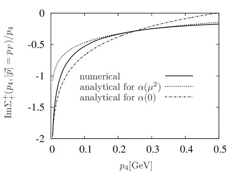
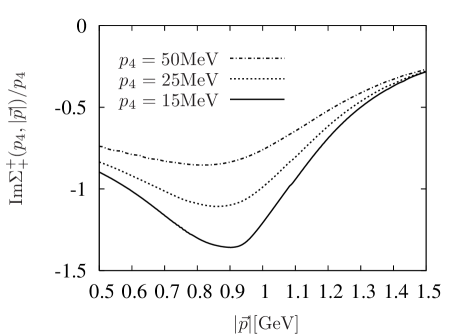
Figure 2: The logarithmic singularity on the Fermi surface as a function of $p_{4}$, compared to the approximation given in eq. (VI) at scales $k=0$ and $k=\mu$, (upper panel) and its momentum dependence for fixed $p_{4}\neq 0$ (lower panel). Here the coupling $\alpha_{I}(k^{2})$ is employed. $\Lambda_{UV}=1.3$GeV is chosen such that the analytical approximation fits the numerical result.

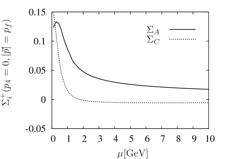
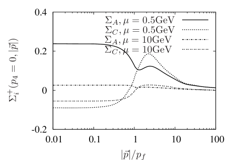
Figure 3: The self energies $\Sigma_{A}^{+}$ and $\Sigma_{C}^{+}$ in the unbroken phase at the Fermi surface as a function of the chemical potential $\mu$ (upper panel) and as a function of the momentum $|\vec{p}|$ for $\mu=0.5\mathrm{GeV}$ and $10\mathrm{GeV}$ for $p_{4}=0$ (lower panel). Note that for $p_{4}=0$ all dressing functions are real.

For completeness, we present numerical results for the self-energy functions $\Sigma_{A}^{+}$ and $\Sigma_{C}^{+}$ in the unbroken phase, see Fig. 3. Displayed are their values at the Fermi surface as a function of the chemical potential $\mu$ and the momentum dependence for $p_{4}=0$ at $\mu=0.5\mathrm{GeV}$ and $10\mathrm{GeV}$. One sees that, in the unbroken phase, the approximation using bare quarks in the medium polarization is justified a posteriori since, as expected, $\Sigma_{A}^{+},\Sigma_{C}^{+}\ll 1$.

VII Results for 2SC and CFL phase in the chiral limit

In this section we combine the presentation of the numerical results for the scalar 2SC and CFL phases for three massless flavors.

The color-flavor structure of the 2SC phase is given by $M=\lambda_{2}\otimes\tau_{2}$ which leads to

$$S^{+\,-1} = S^{+\,-1}_{1}P_{ur,ug,dr,dg}+S^{+\,-1}_{2}P_{ub,db}+S^{+\,-1}_{3}P_{s},$$

$$\Phi^{+} = \frac{Z_{2}}{Z_{1F}}\,\phi^{+}_{2SC}\,\lambda_{2}\otimes\tau_{2}.$$ (78)

Here $(r,g,b)$ and $(u,d,s)$ label color and flavor. The matrices $\lambda_{i}$ and $\tau_{i}$ are the Gell-Mann matrices of color and flavor space, respectively, completed by $\lambda_{0}=\tau_{0}=\sqrt{\frac{2}{3}}\mathds{1}$. As described above, $P_{i}$, denote projectors on the coupled color-flavor space.

The CFL phase is given by the ansatz $M=\lambda_{2}\otimes\tau_{2}+\lambda_{5}\otimes\tau_{5}+\lambda_{7}\otimes\tau_{7}$. Note that $M$ is antisymmetric in color and flavor, respectively. The corresponding condensates can be chosen to be invariant under a $3\otimes\bar{3}=1\oplus 8$ transformation with generators $\tau_{a}-\lambda_{a}^{T}$ Alford:1998mk . Then the matrices $\{P_{i}\}$ turn out to project onto the irreducible representations. We therefore obtain

$$S^{+\,-1} = S^{+\,-1}_{1}P_{1}+S^{+\,-1}_{8}P_{8},$$ (79)

$$\Phi^{+} = \frac{Z_{2}}{Z_{1F}}\left(\phi^{+}_{1}M_{1}+\phi^{+}_{8}M_{8}\right)$$

$$= \frac{Z_{2}}{Z_{1F}}\left(\phi^{+}_{\bar{3}}\sum_{A=\{2,5,7\}}\,\lambda_{A}\otimes\tau_{A}\right.$$

$$\qquad\left.+\,\phi^{+}_{6}\sum_{S=\{0,1,3,4,6,7,8\}}\,\lambda_{S}\otimes\tau_{S}\right),$$

where we have also introduced the commonly used ’antitriplet’ and ’sextet’ pairing function $\phi^{+}_{\bar{3}}=\frac{1}{3}\phi_{1}+\frac{2}{3}\phi_{8}$ and $\phi^{+}_{6}=-\frac{1}{3}\phi_{1}+\frac{1}{3}\phi_{8}$.

Both phases have been studied in a weak coupling analyses in the HDL approximation. Including in this approximation the “normal” quark self energies, the quasiparticle gap at the Fermi surface is given by Wang:2001aq

$$\phi^{+}_{weak,i} = 512\,\pi^{4}\left(\frac{2}{N_{f}g^{2}}\right)^{\frac{5}{2}}e^{-\frac{\pi^{2}+4}{8}}\,\mu\,e^{-\frac{3\pi^{2}}{\sqrt{2}g}}$$ (81)

$$\times\left\{{1\atop 2^{-1/3}}{i=\mathrm{2SC}\atop i=\bar{3}}\right..$$

The momentum dependence takes a more complicated form but for $g^{2}\ln\left(\mu/\phi^{+}_{weak,i}\right)\ll 1$ one can neglect the quark self energies and obtains Wang:2001aq

$$\phi^{+}_{weak,i}\left(\lvert\vec{p}\rvert\right) = \phi^{+}_{weak,i}$$

$$\cos\left(\frac{g}{3\sqrt{2}\pi}\ln\left(\frac{\phi^{+}_{weak,i}}{|p-\mu|+\epsilon_{i}^{+}(p)}\right)\right),$$

with $\epsilon_{i}^{+}(p)^{2}=(p-\mu)^{2}+{\phi^{+}_{weak,i}}^{2}$.

For the weak-coupling approximations of the gap functions displayed in the following figures we use the identical running coupling as the one employed to obtain the displayed numerical solution, respectively. Note, however, that in the strong coupling regime the weak-coupling expressions ceases to be valid.

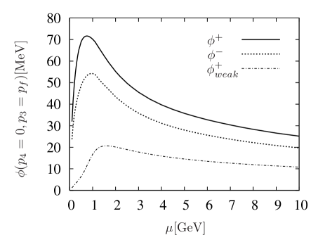
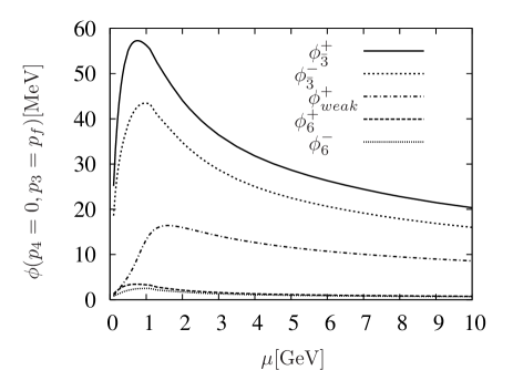
Figure 4: The quasiparticle gaps $\phi^{+}$ and anti-quasiparticle gaps $\phi^{-}$ at the Fermi surface for the 2SC (upper panel) and CFL (lower panel) phases for the coupling $\alpha_{I}(k^{2})$. These are compared to the extrapolated weak coupling result $\phi^{+}_{weak}$.

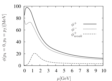
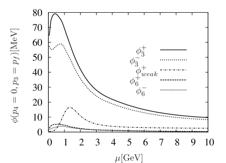
Figure 5: The quasiparticle gaps $\phi^{+}$ and anti-quasiparticle gaps $\phi^{-}$ at the Fermi surface for the 2SC (upper panel) and CFL (lower panel) phases for coupling $\alpha_{II}(k^{2})$. These are compared to the extrapolated weak coupling result $\phi^{+}_{weak}$.

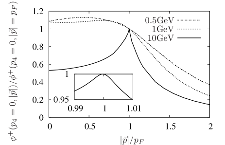
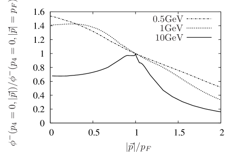
Figure 6: The momentum dependence of the quasiparticle gaps $\phi^{+}$ (upper panel) and anti-quasiparticle gaps $\phi^{-}$ (lower panel) for $p_{4}=0$ normalized to their value at the Fermi surface.

The results for the gap functions at the Fermi surface the for 2SC and CFL phases are shown in Fig. 4 for the coupling $\alpha_{I}(k^{2})$. In Fig. 5 the corresponding results are shown for the coupling $\alpha_{II}(k^{2})$. In both figures it is evident that the extrapolated weak-coupling results for the value of the quasiparticle gap differs by a factor of more than five for $\mu\approx 500\mathrm{MeV}$, resulting in quasiparticle-pairing gaps larger than $50\mathrm{MeV}$. It is worth noting that the results are less sensitive on the coupling than the mass function in the chirally broken phase. This can be attributed to the fact that a stronger coupling also results in stronger screening and damping. In addition, also the anti-quasiparticle gap function are determined self-consistently. Nevertheless, it is remarkable that the ratio of the 2SC and anti-triplet CFL gaps is almost equal to $2^{1/3}$ as in the weak coupling analysis. The reason for this behavior is that the normal self energies $\Sigma^{+}_{i}$ are only weakly modified compared to the self energies in the unbroken phase. This amounts to an effective “decoupling” of normal self energies and gap functions, and thus the factor $2^{1/3}$ is directly inherited from the pairing pattern in color-flavor space.

As can be inferred from Fig. 3 and the estimate given in eq. (53), the energy gap in the excitation spectrum $\Delta_{i}^{e}$ is at most $15\%$ smaller than the gap function at the corresponding kinematical point. (Note that the corresponding coefficients $\delta_{i}$ in the decomposition of $M^{\dagger}M$ are given by: $\sqrt{\delta_{2SC}}=\sqrt{\delta_{1}}=1$ and $\sqrt{\delta_{8}}=2$.) We also emphasize, that $\phi^{+}(p)\rightarrow\phi^{-}(p)$ for $\mu\rightarrow 0$, which can be non-zero, indicating a Bose-Einstein condensation of diquarks. This is found for the coupling $\alpha_{II}(k^{2})$. However, this is not expected to be the energetically favored state in the vacuum, since spontaneous chiral symmetry breaking has not been taken into account here.

In Fig. 6 we present the momentum dependence of the quasiparticle gaps $\phi^{+}$ and anti-quasiparticle gaps $\phi^{-}$ for $p_{4}=0$ for several chemical potentials, obtained with the coupling $\alpha_{I}(k^{2})$. For large values of $\mu$ the gap function is concentrated around the Fermi surface and the quasiparticle gaps show a cosine-like behavior near the maximum. However, at chemical potentials of the order $\Lambda_{QCD}$, the Fermi surface is no longer the main contributing region to the gap integral, and even the maximum of the gap function is no longer on or close to the Fermi surface.

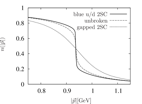
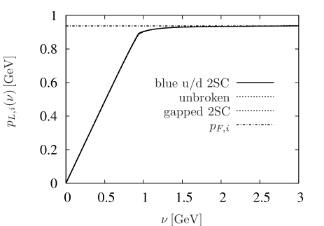
Figure 7: The occupation numbers (upper panel) and the function defined in eq. (83), $p_{L,i}(\nu)$, (lower panel) for the different quark channels in the 2SC phase at $\mu=1\mathrm{GeV}$ with the coupling $\alpha_{I}(k^{2})$. As can be seen in the panels all Fermi momenta are (almost) equal and given by $p_{F,i}\approx.937\mathrm{GeV}$, c.f. the dashed-dotted line in the lower panel. The lines of the different channels are nearly indistinguishable.

As described in sect. IV.1, the occupation numbers of the quasiparticles are calculated from the normal propagators. These are displayed in the upper panel of Fig. 7 for the 2SC phase, employing the coupling $\alpha_{I}(k^{2})$. The occupation number of the gapped red and green $u$- and $d$-quarks is, as expected and due to the pairing, a smooth function around the Fermi momentum. On the other hand, the occupation number of the blue $u$- and $d$-quarks changes rapidly. Within the present approximation, i.e. neglecting quark self energies in the medium polarization, these quarks are in a state at the borderline between a Fermi and a non-Fermi liquid.

The decoupled $s$-quarks are in the unbroken phase and one clearly sees, especially when comparing to the blue $u$- and $d$-quarks, that the occupation number changes smoothly. As already mentioned, this is another feature of non-Fermi liquids which, strictly speaking, indicates the breakdown of the quasiparticle picture. We also find a significant depletion at $|\vec{p}|=0$ due to the interaction.

The density can either be obtained by integration of the occupation numbers or via the Luttinger theorem (see sect. V). The conditions for the latter are fulfilled since all self-energies are real for $p_{4}=0$. To analyze this remarkable feature we define the function

$$p_{L,i}(\nu) = \left(3\int_{0}^{\nu}dqq^{2}n_{i}(q)\right)^{\frac{1}{3}},$$ (83)

which has to obey the limiting behavior $\lim_{\nu\rightarrow\infty}p_{L,i}(\nu)=p_{F,i}$. From Fig. 7 one sees that this limit is assumed for $\nu>p_{F,i}$, and that the expectation derived from Luttinger’s theorem is nicely fulfilled within the numerical accuracy . Note also that all Fermi momenta are very close to each other, a fact which justifies a posteriori the approximation of neglecting the neutrality conditions.

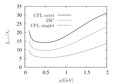
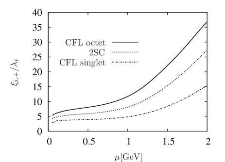
Figure 8: The ratio between the coherence length and mean-free path in 2SC and CFL phase for the coupling $\alpha_{I}(k^{2})$ (upper panel) and $\alpha_{II}(k^{2})$ (lower panel).

It is instructive to compare the coherence length of the diquarks, $\xi_{+}$, to the mean-free path as determined from the density. The results are shown in Fig. 8 as a function of the chemical potential. Although the two different couplings lead to a distinctive pattern for these ratios it is safe to conclude that the size of a Cooper pair at moderate chemical potentials, $\mu\approx 500\mathrm{MeV}$, is only several times the mean-free path, the precise value depending on the diquark channel and the employed coupling (similar results were already presented in ref. Abuki:2001be for the 2SC phase.). Although there is an analogy to the crossover between a BCS-type superconductor in weak coupling to the strongly coupled regime (Bose-Einstein condensate) the size of the diquarks suggest that the 2SC and CFL phases resemble a strongly coupled BCS system. However the result indicates, that mean-field approximations are very questionable. In the limit $\mu\rightarrow 0$, we again find a different behavior for the two employed couplings indicating Bose-Einstein condensation of diquarks for $\alpha_{II}(k^{2})$ for very small chemical potentials.

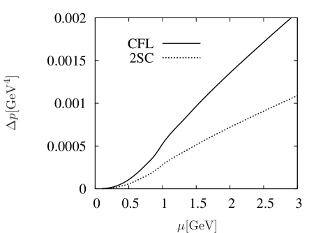
Figure 9: The pressure difference between the superconducting phases (2SC and CFL) and the unbroken phase employing $\alpha_{I}(k^{2})$.

Finally, the pressure difference between the superconducting phases (2SC and CFL) and the unbroken phase are displayed in Fig. 9. This quantity is given by the negative effective action difference, and is here calculated within the approximate CJT formula given in eq. (IV.2). In the chiral limit, the CFL phase is the most favored phase, as expected. This is in good qualitative agreement with the parameterized form

$$\Delta p = \sum_{i}\mathrm{rank}(P_{i})\,\frac{p_{F,i}^{2}\,\Delta^{+\,2}_{i}}{8\pi^{2}}\,.$$ (84)

which is (slightly) a generalized formula as compared to the one obtained in the weak coupling regime Schmitt:2004et .

VIII Conclusions and outlook

We have presented the solution of a truncated Dyson-Schwinger equation for the quark propagator at non-vanishing chemical potential in the chiral limit. The truncation includes the in-medium modification of the gluon propagator and has been chosen such that, at vanishing density, known results for the vacuum and at asymptotically high densities the corresponding weak-coupling expressions are recovered. We have determined analytically the ultraviolet behavior, i.e. the anomalous dimensions, of the gap functions.

The most remarkable feature of these self-consistent solutions are the values of the gap functions: The quasiparticle-pairing gaps are several times larger than the extrapolated weak-coupling results even for sizeable chemical potentials $\mu\approx 1$GeV. This is true irrespective of the considered phase (2SC or CFL) and the employed running coupling.

The investigation, presented here, provides the starting point for more realistic studies involving finite current masses. Using different quark masses the question of implementing neutrality conditions (which could be ignored here) becomes important.

Due to solutions of the gluon- and ghost Dyson-Schwinger equations at non-vanishing temperatures Maas an investigation of different regions of the phase diagram opens up. However, to solve the complete coupled system of the Dyson-Schwinger equations for the QCD propagators remains a challenge. A study of the question of deconfinement due to a non-vanishing quark density requires certainly also a better understanding of the infrared behavior of these Green’s functions and thus an infrared analysis of the coupled Dyson-Schwinger system at non-vanishing temperatures and densities.

References

- (1) K. Rajagopal and F. Wilczek, arXiv:hep-ph/0011333; T. Schafer, arXiv:hep-ph/0304281; M. Buballa, Phys. Rept. 407, 205 (2005) [arXiv:hep-ph/0402234]; I. A. Shovkovy, arXiv:nucl-th/0511014.
- (2) D. H. Rischke, Prog. Part. Nucl. Phys. 52, 197 (2004) [arXiv:nucl-th/0305030].
- (3) D. T. Son, Phys. Rev. D 59, 094019 (1999) [arXiv:hep-ph/9812287]. T. Schafer and F. Wilczek, Phys. Rev. D 60, 114033 (1999) [arXiv:hep-ph/9906512]; D. K. Hong, V. A. Miransky, I. A. Shovkovy and L. C. R. Wijewardhana, Phys. Rev. D 61, 056001 (2000) [Erratum-ibid. D 62, 059903 (2000)] [arXiv:hep-ph/9906478]; I. A. Shovkovy and L. C. R. Wijewardhana, Phys. Lett. B 470, 189 (1999) [arXiv:hep-ph/9910225].
- (4) M. G. Alford, K. Rajagopal and F. Wilczek, Phys. Lett. B 422, 247 (1998) [arXiv:hep-ph/9711395]; R. Rapp, T. Schafer, E. V. Shuryak and M. Velkovsky, Phys. Rev. Lett. 81, 53 (1998) [arXiv:hep-ph/9711396].
- (5) J. Greensite, Prog. Part. Nucl. Phys. 51, 1 (2003) [arXiv:hep-lat/0301023].
- (6) J. Greensite, S. Olejnik and D. Zwanziger, AIP Conf. Proc. 756, 162 (2005) [arXiv:hep-lat/0411032].
- (7) D. Zwanziger, Phys. Rev. D 70, 094034 (2004) [arXiv:hep-ph/0312254].
- (8) L. von Smekal and R. Alkofer, in: Proceedings of the Fourth International Conference on Quark Confinement and the Hadron Spectrum (CONFINEMENT IV), July 3-8, Vienna [arXiv:hep-ph/0009219].
- (9) D. Zwanziger, Phys. Rev. Lett. 90, 102001 (2003) [arXiv:hep-lat/0209105].
- (10) A. Nakamura and T. Saito, arXiv:hep-lat/0512042.
- (11) R. Alkofer, M. Kloker, A. Krassnigg and R. F. Wagenbrunn, Phys. Rev. Lett. 96, 022001 (2006) [arXiv:hep-ph/0510028].
- (12) P. J. Silva and O. Oliveira, arXiv:hep-lat/0511043.
- (13) A. Sternbeck, E. M. Ilgenfritz, M. Mueller-Preussker and A. Schiller, Phys. Rev. D 72, 014507 (2005) [arXiv:hep-lat/0506007].
- (14) C. S. Fischer and H. Gies, JHEP 0410, 048 (2004) [arXiv:hep-ph/0408089].
- (15) J. M. Pawlowski, D. F. Litim, S. Nedelko and L. von Smekal, Phys. Rev. Lett. 93, 152002 (2004) [arXiv:hep-th/0312324].
- (16) R. Alkofer, W. Detmold, C. S. Fischer and P. Maris, Phys. Rev. D 70, 014014 (2004) [arXiv:hep-ph/0309077].
- (17) A. Maas, B. Gruter, R. Alkofer and J. Wambach, arXiv:hep-ph/0210178; A. Maas, J. Wambach, B. Gruter and R. Alkofer, Eur. Phys. J. C 37, 335 (2004) [arXiv:hep-ph/0408074]; B. Gruter, R. Alkofer, A. Maas and J. Wambach, Eur. Phys. J. C 42, 109 (2005) [arXiv:hep-ph/0408282]; A. Maas, J. Wambach and R. Alkofer, Eur. Phys. J. C 42, 93 (2005) [arXiv:hep-ph/0504019]; A. Maas, Mod. Phys. Lett. A 20, 1797 (2005) [arXiv:hep-ph/0506066].
- (18) C. S. Fischer and R. Alkofer, Phys. Rev. D 67, 094020 (2003) [arXiv:hep-ph/0301094].
- (19) Q. Wang and D. H. Rischke, Phys. Rev. D 65, 054005 (2002) [arXiv:nucl-th/0110016].
- (20) L. P. Gorkov, Sov. Phys. JETP 9 (1959) 1364; Y. Nambu, Phys. Rev. 117 (1960) 648.
- (21) R. Alkofer and L. von Smekal, Phys. Rept. 353, 281 (2001) [arXiv:hep-ph/0007355].
- (22) C. D. Roberts and S. M. Schmidt, Prog. Part. Nucl. Phys. 45, S1 (2000) [arXiv:nucl-th/0005064].
- (23) D. H. Rischke, Phys. Rev. D 62, 054017 (2000) [arXiv:nucl-th/0003063].
- (24) A. Gerhold and A. Rebhan, Phys. Rev. D 68, 011502 (2003) [arXiv:hep-ph/0305108].
- (25) D. D. Dietrich and D. H. Rischke, Prog. Part. Nucl. Phys. 53, 305 (2004) [arXiv:nucl-th/0312044].
- (26) M. Buballa and I. A. Shovkovy, Phys. Rev. D 72, 097501 (2005) [arXiv:hep-ph/0508197].
- (27) C. S. Fischer and R. Alkofer, Phys. Lett. B 536, 177 (2002) [arXiv:hep-ph/0202202]; C. S. Fischer, B. Gruter and R. Alkofer, Ann. Phys. (2006), in print [arXiv:hep-ph/0506053].
- (28) P. O. Bowman, U. M. Heller, D. B. Leinweber, M. B. Parappilly and A. G. Williams, Phys. Rev. D 70, 034509 (2004) [arXiv:hep-lat/0402032].
- (29) F. J. Llanes-Estrada, C. S. Fischer and R. Alkofer, arXiv:hep-ph/0407332.
- (30) J. I. Skullerud, P. O. Bowman, A. Kizilersu, D. B. Leinweber and A. G. Williams, Nucl. Phys. Proc. Suppl. 141, 244 (2005) [arXiv:hep-lat/0408032].
- (31) H. W. Lin, arXiv:hep-lat/0510110.
- (32) M. S. Bhagwat, M. A. Pichowsky, C. D. Roberts and P. C. Tandy, Phys. Rev. C 68, 015203 (2003) [arXiv:nucl-th/0304003].
- (33) C. S. Fischer and M. R. Pennington, Phys. Rev. D 73, 034029 (2006) arXiv:hep-ph/0512233.
- (34) J. I. Kapusta, Finite-temperature field theory (Cambridge University Press, Cambridge, 1993).
- (35) C. Manuel, Phys. Rev. D 62, 114008 (2000) [arXiv:hep-ph/0006106].
- (36) R. D. Pisarski and D. H. Rischke, Phys. Rev. D 60, 094013 (1999) [arXiv:nucl-th/9903023].
- (37) V. P. Gusynin and V. A. Miransky, Phys. Lett. B 191, 141 (1987).
- (38) C. D. Roberts and A. G. Williams, Prog. Part. Nucl. Phys. 33, 477 (1994) [arXiv:hep-ph/9403224].
- (39) J. M. Cornwall, R. Jackiw and E. Tomboulis, Phys. Rev. D 10, 2428 (1974).
- (40) A. Schmitt, Phys. Rev. D 71, 054016 (2005) [arXiv:nucl-th/0412033].
- (41) C. Manuel, Phys. Rev. D 62, 076009 (2000) [arXiv:hep-ph/0005040].
- (42) T. Schafer and K. Schwenzer, Phys. Rev. D 70, 054007 (2004) [arXiv:hep-ph/0405053].
- (43) M. G. Alford, K. Rajagopal and F. Wilczek, Nucl. Phys. B 537, 443 (1999) [arXiv:hep-ph/9804403].
- (44) H. Abuki, T. Hatsuda and K. Itakura, Phys. Rev. D 65, 074014 (2002) [arXiv:hep-ph/0109013].